Surveillance Video Synopsis in GIS


1
Key Laboratory of Virtual Geographic Environment (Nanjing Normal University), Ministry of Education, Nanjing 210023, China
2
State Key Laboratory Cultivation Base of Geographical Environment Evolution (Jiangsu Province), Nanjing 210023, China
3
Jiangsu Center for Collaborative Innovation in Geographical Information Resource Development and Application, Nanjing 210023, China
*
Authors to whom correspondence should be addressed.
ISPRS Int. J. Geo-Inf. 2017, 6(11), 333; https://doi.org/10.3390/ijgi6110333
Submission received: 14 August 2017
/
Revised: 23 October 2017
/
Accepted: 26 October 2017
/
Published: 31 October 2017
(This article belongs to the Special Issue State-of-the-Art Virtual/Augmented Reality and 3D Modeling Techniques for Virtual Urban Geographic Experiments)
Abstract
:Surveillance videos contain a considerable amount of data, wherein interesting information to the user is sparsely distributed. Researchers construct video synopsis that contain key information extracted from a surveillance video for efficient browsing and analysis. Geospatial–temporal information of a surveillance video plays an important role in the efficient description of video content. Meanwhile, current approaches of video synopsis lack the introduction and analysis of geospatial-temporal information. Owing to the preceding problems mentioned, this paper proposes an approach called “surveillance video synopsis in GIS”. Based on an integration model of video moving objects and GIS, the virtual visual field and the expression model of the moving object are constructed by spatially locating and clustering the trajectory of the moving object. The subgraphs of the moving object are reconstructed frame by frame in a virtual scene. Results show that the approach described in this paper comprehensively analyzed and created fusion expression patterns between video dynamic information and geospatial–temporal information in GIS and reduced the playback time of video content.
1. Introduction
Surveillance cameras are globally used, and a considerable amount of surveillance videos are collected daily. Surveillance data are extensively used in many fields, such as security, transportation, and environmental monitoring for data analysis, status detection, abnormality warning, and other related functions. Video surveillance data are characterized by a considerable amount of data with sparsely distributed valuable information, which hinders effective real-time analysis of video data. Video synopsis construction [1] is a commonly used method for extracting valuable information from massive video data. Video synopsis is implemented via moving object detection and tracking technology [2,3], efficient extraction of dynamic video information, analysis and expression through intensive storage of moving objects, and foreground and background reorganization of video scenes. Current methods for video synopsis creation focus on the analysis of video images, but geospatial–temporal information should also be applied. Surveillance cameras have spatial association with a geographic scene [4] by storing information of spatial–temporal properties within a geographic space. Although geospatial–temporal information independently exists from video images, a few sections, such as video location, camera visual field, and geospatial direction, play important roles in the effective and complete description of the video content [5]. Introducing geospatial–temporal information as key video information in the extraction and analysis of valuable information for video synopsis is necessary. Geospatial–temporal information comes from a virtual geographic environment (VGE), which is a type of web- and computer-based geographic environment built for geographic understanding and problem solving. Emphasizing the linkage between our method and VGE is necessary. Specifically, by merging geographic knowledge, computer technology, virtual reality technology, network technology, and geographic information technology, VGE is built with the objective of providing open, digital windows into geographic environments in the physical world to allow users to “feel it in person” by augmenting the senses and “know it beyond reality” through geographic phenomena simulation and collaborative geographic experiments. Considering the above characteristics of VGE, we put forward a method for surveillance video synopsis in the geographical scene that combines video information and geographic scene. This method will help users quickly and efficiently understand the geographical processes reflected in surveillance videos and simultaneously create a technological basis for analyzing moving video objects and other geographical objects.
The process of video synopsis includes filtration of key video contents [6], extraction of dynamic video information [7], storage and analysis [8], and reorganization and expression [1]. Among these processes, supporting geospatial information is necessary to analyze geographic content in a video. Reorganization and expression of video data must integrate geospatial information to accurately reconstruct the geospatial–temporal movement of an object and the position of a video event. However, the analysis of key contents of the original video storage lacks consideration of geospatial–temporal information and is not introduced in the analysis and storage process. The reorganization of the dynamic video information is realized in the image space. Hence, effective description and analysis of geospatial–temporal information cannot be carried out. In summary, existing video synopsis approaches ignore the importance of geospatial–temporal information in enhancing the integrity of video synopsis, as well as its lack of capability to create fusion expression patterns for video and geospatial–temporal information. Therefore, constructing a new video synopsis approach that can effectively integrate geospatial–temporal information, enhance the integrity of video synopsis, and assist users’ understanding of contents within a geographic scene is necessary.
In this paper, a new approach on video synopsis with geospatial information expression capability is constructed using the VideoGIS platform. The VideoGIS platform integrates video-image processing system and GIS to establish environmental sensing and analysis and supports related functions, such as organization and management of video data [9], fusion expression [10], and spatial–temporal analysis [11,12] under a unified geographic reference. Based on our previous research on the integration of video moving objects and GIS [13], this paper expands the application of the integration by attempting to use virtual geographic scene model as the visualization platform for video synopsis. The process of our video synopsis is shown as follows. First, based on the extraction and geospatial positioning of video moving objects, a storage model is constructed to establish the integration of GIS and video moving objects. Then, a virtual visual field is constructed by using a virtual geographic scene as the background and the fusion expression pattern between this background and the subgraphs of video moving objects [14,15]. Finally, the spatial–temporal position and display order of video moving objects are optimized based on the geospatial clustering of their trajectories to create a video synopsis.
The organizational structure of this paper is as follows: Section 2 denotes an overview of related work; Section 3 describes the processing flow and related technical details of the surveillance video synopsis in GIS; In Section 4, the visualization effect and the time-reducing performance of the video synopsis are discussed and analyzed by the experimental results; and Section 5 summarizes and concludes the paper.
2. Related Work
Surveillance video synopsis in GIS is carried out through the geo-specialization of surveillance video, which is executed by storage and fusion expression of video moving objects. In this section, we introduce related work in four aspects: video moving objects storage, fusion of GIS and video, classification of video synopsis, and optimization of video moving object expression in video synopsis.
The storage model of video moving objects is created to define the information of moving objects that needs to be stored, thereby providing a basis for further analysis. The method of Ji et al. [16] is simple; their model only stores image coordinates of the center point in every moving object subgraph per video frame, and these image coordinates are recorded as the trajectory of the moving object. Puletic et al. [6] recorded the spatial–temporal trajectory information of a single moving object as follows: object number, spatial position, outer border length and width, and number of pixels in the subgraph of an object. Apart from object number, information was recorded frame-by-frame. Sun et al. [17] defined the elements of a moving object storage model as follows: time of appearance, the set of outer borders, the set of spatial–temporal trajectories, and the set of motion velocities. Chiang et al. [18] defined the storage model as initial time, time of disappearance, occurrence of video frame group, the minimum width and height of circumscribed rectangles in an object, and the area of object subgraph. Chen et al. [19] also proposed the following record model to address the problems related to the extraction of spatial–temporal position of moving objects in a camera network: object number, object entry and exit time, trajectories of the object captured by the multiple cameras, appearance of the objects, and topological relationship of the camera network.
The purpose of fusion between video and GIS is to uniformly express video information from different geographical locations. The realization method fuses video and GIS according to a virtual scene model, in which video information is displayed in a geospatial position inside the visual field of a camera [20,21]. According to the differences of mapping modes, the fusion method in surveillance video and virtual scene is divided into two categories: GIS-video image fusion and GIS-video object fusion. GIS-video image fusion directly shows the video image according to camera parameters in the corresponding position of a virtual scene [22]. This fusion method is easily implemented, but lacks analysis of video contents, which results in insufficient information on video–GIS integration. GIS-video object fusion combines video background and video moving objects in a geographic space [23]. Based on the differences of video moving objects formation in a virtual scene, GIS-video object fusion can be divided into different subclasses, such as foreground and background scene independent projection [14,24], foreground projection [15], and foreground abstract projection [25].
Different kinds of video synopses are mainly divided into three categories according to their fusion expression patterns: static video synopsis, dynamic video synopsis, and mixed video synopsis. Static video synopsis [26,27] combines moving object subgraphs from key frames into static background images. Dynamic video synopsis is classified into paragraph splicing and object fitting. Paragraph splicing [28,29] splits spatial–temporal pixels into different video image areas from different time passages to create a short video as video synopsis. Object fitting [30,31] dynamically adapts moving object subgraphs to the video background to create a short video synopsis. Mixed video synopsis [17] is a combination of static and dynamic video synopsis. This method uses static video synopsis for video segmentation and dynamic video synopsis for video content description in each sub-paragraph. In summary, the current approaches on video synopsis use rasterized images as the display platform for frame interception or dynamic information re-combination in the original video and generate a multi-map or a short video.
Display optimization of moving objects in a video synopsis includes the optimization of the moving objects’ ontology, display sequence, and spatial–temporal position. Ontology optimization of a moving object improves its generating efficiency in a video synopsis. This optimization is typically performed through the hybrid coding method [32], compressed domain reconstruction method [33], and parallel method to accelerate read access in moving object information [34]. Optimization of the moving object display sequence improves the order and display duration of the moving objects in a concentrated expression process and helps to understand the temporal structure and interaction of the moving objects in the original video. Typical methods for display sequence optimization include the multi-constraint conditional ordering method [1] and the timeline correction method [35]. Optimization of the moving objects’ spatial-temporal position reduces the display collision of moving objects during concentrated expression. Typical methods for spatial–temporal positioning optimization include the sub-channel offset method [36] and the moving area expansion method [37]. Under many circumstances, ontology optimizations of moving objects and display sequence simultaneously exist. A few methods create unified processing of the two optimizations, such as methods based on maximum posteriori probability estimation [38], energy minimization equation [39,40], and set theory [41]. The preceding methods are carried out based on the mathematical models to optimize the location and occurrence time of moving objects in a video and account for the temporal structure and spatial correlation of the moving objects in a video synopsis.
3. Surveillance Video Synopsis in GIS
Surveillance video synopsis in GIS is implemented based on the integration of moving objects and GIS. This section describes the main process of surveillance video synopsis in GIS and provides details for the technical implementation of each step (as shown in Figure 1), including georeferencing and clustering of moving objects, virtual field construction, moving object display trajectory generation, and moving object expression.
3.1. Extraction and Clustering of Moving Objects
Video synopsis expresses moving objects in a short period of time. The trajectories of moving objects are cluttered and random. The expression of the subgraphs of moving objects in a virtual scene causes problems, such as subgraph crowding, confusion, and other issues, which hinder users’ effective understanding of video content. The expression of moving objects should be simplified to provide visual-friendly video synopsis results. According to the extraction and spatial mapping of the trajectories of moving objects, trajectories are classified according to the geospatial direction of their entries and exits in the field of view of cameras. Trajectories with similar geospatial directions are then clustered and used as the basis for the construction of video synopsis.
3.1.1. Extraction of Moving Objects
The content of extracted information on moving objects includes spatial–temporal information and sub-graphs in video frames. The specific steps include moving object detection, tracking, and storage.
As our video synopsis method is implemented in an outdoor scene, the video background is relatively stable. Therefore, the background subtraction method is used for moving object detection. The background subtraction method makes use of the subtraction image between the current and the background image to detect moving objects. The key is to learn to build the background model. The background model is defined as B, and the set of grayscale maps for video images is defined as V:
where Zt denotes the gray-scale map for a video frame image. The background model B is initialized as follows:
V = {Z1, …, Zt},
By learning from each video frame image, the background model B is recursively updated as follows:
where Bt denotes the updated result of the background model after adaptive learning from the tth video frame image in the learning rate as α(α∈{0,1}⊂R). After completing the learning from all video frame images, the video background model B is substituted by Bt. The subtraction In between each video frame image Zn and background model B is considered the foreground region:
when the foreground region In is obtained from different video frames, we use the blob-based tracking algorithm to track each moving object [42]. We obtain the attributes of the moving object, such as moving speed, position, motion trajectory, and acceleration [43]. Subsequently, the corresponding storage model is constructed to record the moving object information. The general representation of the moving object storage model is shown as follows:
where O denotes the set of information of a moving object, and C denotes the set of position information of the moving object in each frame. F denotes the sub-image in each frame of the moving object, the relevant attributes, and other collected data. f1i, f2i, … denote the moving objects in each frame with different characteristics. S comprises all moving object subgraphs within a period of time. I(i,j) denotes a single moving object subgraph in the jth frame of the ith moving object.
Bt = (1 − α)β(t − 1) + αZt,
In = Zn − B.
O = {C, F, S},
C = {(xi, yi)(i = 1, 2, …, n)},
F = {(f1i, f2i…)(i = 1, 2, …, n)},
S = {I(i,j),(i = 1, 2, …, N),(j = 1, 2, …, n)},
The detection, tracking, and storage of the moving object are implemented in the openCV runtime library, which has been integrated in the VideoGIS platform.
3.1.2. Georeferencing of Moving Object Trajectory
The geospatial mapping matrix of the image should be constructed to effectively mark the trajectory in the geographic space [44]. Based on the assumption that the ground in the camera’s visual field is flat, we denote the mapping matrix as M. The trajectory of the moving object is mapped onto the geographic space through M, and the moving object trajectory is set as Taj:
where Ti denotes the geospatial trajectory of each moving object, ti denotes each geospatial coordinate of the spatio–temporal sampling point of the moving object, N denotes the number of moving objects, and n denotes the number of sampling points of a single moving object. Obtaining Taj requires the construction of mapping model M, which could map the moving object trajectory Tajimg from the image space to the geographical space:
Taj = {Ti, (I = 1, 2, …, N)},
Ti = {ti (X(i,j),Y(i,j) ),(j = 1, 2, …, n)},
Taj = M ∙ Tajimg.
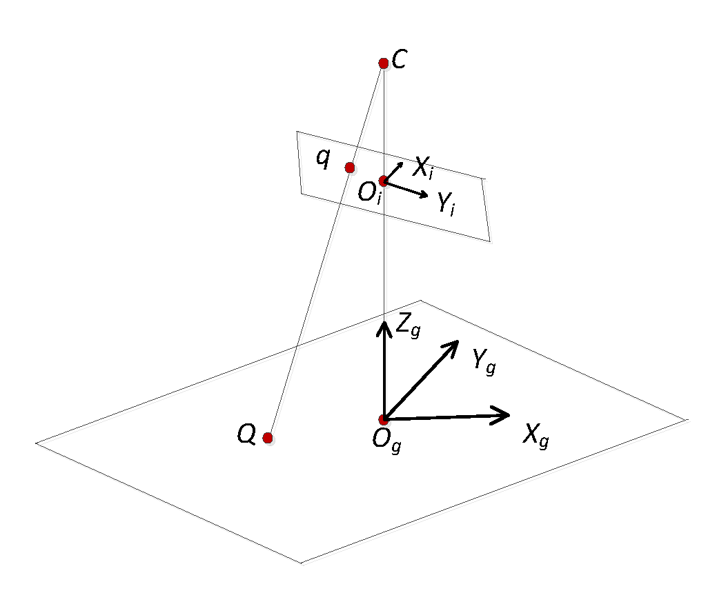
The mapping model M is established using the homography matrix method. The relationship between the geospatial coordinate system and the image space coordinate system is shown in Figure 2. The center of the station is denoted by C, the image space coordinate system is denoted by Oi, Xi, Yi, and the geospatial coordinate system is denoted by Og, Xg,Yg, Zg.
Based on the assumption that q is a point in the image spatial coordinate system, Q is a point in the geographic coordinate system, q and Q are a pair of points with the same name:
q = [x y 1]T,
Q = [X Y 1]T.
Let the homography matrix be M such that the relationship between q and Q is:
q = MQ.
M is represented as follows:
M has six unknowns; thus, at least three pairs of image and geospatial points should be determined to solve M. When M is determined, the coordinates of any point in the geographic space can be solved:
3.1.3. Clustering of Moving Object Trajectories
Classifying the trajectories prior to video synopsis is necessary to distinguish the moving object trajectories with different geographical directions. We employ the QT clustering method instead of prior knowledge classification to facilitate the application of the trajectory classification results to different scenes. The QT clustering method does not need a pre-specified number of clusters.
In this paper, the geospatial location of the entrance and exit of the trajectory is selected as the clustering target. The set of moving object trajectories Ψ is solved based on moving object trajectories, Ti. For ∀Ti, we mark its entry/exit point as t(i,0)/t(i,n), and the center point of the camera’s quadrilateral view as tcen. We still mark all trajectory entries as ten and all trajectory exits as tex, which are defined as follows:
ten = {t(i,0),(i = 1, 2, …, N)},
tex = {t(i,n),(i = 1, 2, …, N)}.
As shown in Figure 3, the angle α between the two exit/entry points t(i1,0), t(i2,0) of two moving objects and the center point of the camera’s quadrilateral view tcen is used as the track entry/exit similarity measurement between different trajectories. This angle could effectively set the object trajectories with similar geographical directions and movement trends into the same cluster. The elements in ten and tex are clustered. α is defined as follows:
α = cos−1∠(tcen, t(i1,0) ,t(i2,0)).
The clustering radius angle threshold is denoted as αthr. We use the QT clustering algorithm [45] to cluster trajectory entries and exits. Finally, the trajectory entry and exit clusters are obtained as Ψen and Ψex, respectively. Clusters Ψen and Ψex are matched with the trajectory of the same number. The set of moving object trajectories Ψ is defined as follows:
where κ denotes the number of trajectories obtained in the matching of clusters, and ρ denotes the number of trajectory elements in the εth class. Based on trajectory clustering, the expression of the moving object subgraph set S changes to the following form:
where Sλ denotes the set of all moving object subgraphs in the λth trajectory cluster, S(λ,ε) denotes the subgraph set of the εth moving object in the λth trajectory cluster, and υε denotes the number of subgraphs for a single moving object.
Ψ = {cλ,(cλ = {Tε,(ε = 0, …, ρ)},(λ = 1, 2, …, κ))},
3.2. Video Synopsis in Virtual Scene
The following steps are necessary to distinguish the moving objects from different clusters and show the geographic direction of the moving object trajectories in the process of video synopsis: generating the virtual field of vision, constructing the trajectory fitting centerline, taking the trajectory cluster with the geography direction as the basic expression unit, and constructing a specific expression model for video synopsis expression in a virtual geographic scene.
3.2.1. Virtual Field of Vision Generation
The virtual field of vision, which includes the geospatial horizon generation and virtual perspective generation of the camera, should be generated to fully and accurately express video synopsis in a virtual geographic scene.
The method of camera geospatial horizon generation is as follows. Based on the mapping matrix M and the assumption of flat ground in the horizon of the camera, the four corner points in an image space, namely b1(0, 0), b2(xmax, 0), b3(0, ymax), and b4(xmax, ymax), are obtained by substituting the corresponding geospatial mean points as B1(X1,Y1,Z0), B2(X2,Y2,Z0), B3(X3,Y3,Z0), and B4 (X4,Y4,Z0), respectively. The area surrounded by the plane quadrilateral B1B2B3B4 is the camera geospatial horizon.
Local visualization of the virtual scene dynamically represents moving objects through virtual perspective generation. The virtual scene view selection method is shown as follows. Based on the geospatial position and altitude of the surveillance camera, visual effects are created by selecting the appropriate virtual camera position and viewing angle in the virtual scene. Through field measurement of the scene elevation Z0 and the geospatial position of the camera, tcam = (Xcam,Ycam,Zcam) is obtained. From the mapping matrix M, the mean point tcen = (Xcen,Ycen,Z0) of the center point of the image in the geographic scene is obtained. The viewing angle of the virtual scene is denoted as view field angle (VFA). The minimum value of VFA as VFAmin (as shown Figure 4) should be determined to ensure that the view of the camera is included in the virtual scene:
where bi denotes the edge point of the horizon polygon, tcam denotes the camera locator in the virtual scene, and vector (tcam, tcen) denotes the centerline of the virtual camera. The scene view angle VFA is (VFA ≥ VFAmin), and the virtual perspective is displayed in the geographic scene as the background of video synopsis.
VFAmin = 2 × cos(−1)∠(tcen, tcam, tm),
tm = Max(dist(bi, tcen),(i = 1, 2, 3, 4)),
3.2.2. Trajectory Fitting Centerline Generation
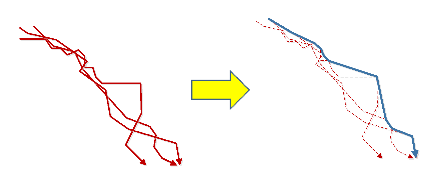
The trajectory fitting centerline method is applied and used as the common display trajectory to express moving objects from the same cluster and differentiate the moving objects from different trajectory clusters.
The trajectory cluster number is denoted as λ. The number of the moving object ε is sequentially taken from 0 to ρ to obtain the set of subgraphs as {S(λ,0), …, S(λ,ρ)}. Then, the number of subgraph j is sequentially taken from 0 to υε in each subgraph set I((λ,ε),j) and displayed in a virtual scene. By completing the construction of the trajectory cluster fitting centerline, the moving object subgraphs are dynamically displayed on the trajectory fitting centerline. The method is carried out as follows: each moving object trajectory cluster is marked as cλ and the corresponding fitting centerline as PLλ, as shown in Figure 5. PLλ is defined as follows:
where t(λ,start) is denoted as the start point of the center line, t(λ,end) is denoted as the end point of the fitting centerline, and cofλ is denoted as the fitting centerline polynomial coefficient set. Factor σ(λ,i) is denoted as the fitting polynomial coefficient set, and Ο is denoted as the order of the fitting polynomial. Factors t(λ,start) and t(λ,end) are obtained by calculating the gravity of all the entries and exits in each trajectory cluster:
where is obtained by the least squares polynomial fitting of the geospatial position of each sampling point in each trajectory for the current trajectory cluster. Variable is defined as follows:
where ρ is the number of elements for the trajectory cluster cλ. The elements σ(λ,ε,i) in the trajectory fitting coefficients cof(λ,ε) and elements σ(λ,i) of the corresponding fitting centerline polynomial are obtained. Then, the fitting centerline coefficients cofλ are obtained:
PLλ = {t(λ,start),t(λ,end), cofλ},
cofλ = {σ(λ,i),(i = 1, …, Ο)},
cof(λ,ε) = {σ(λ,ε,i) (i = 1, …, Ο)},(ε = 0, …, ρ),
3.2.3. Expression of Video Moving Object
During the display of the moving object subgraph I((λ,ε),j), display position should be considered in the virtual geographic scene and in the display synchronization between subgraphs from different moving objects. For each moving object subgraph I((λ,ε),j), we denote P((λ,ε),j) as its position in the virtual geographic scene. P((λ,ε),j) is calculated as follows:
where λ denotes the number of trajectory cluster, N denotes the number of sampling points displayed on the cluster fitting centerline, υ denotes the number of moving object subgraphs, j denotes the number of subgraphs for the specified moving object, and [...] denotes the left rounding process.
P((λ,ε),j) = (X(λ,n),Y(λ,n)),
n = [(N × j/υ)],
Different video moving objects must be synchronously displayed to reduce display frames and enhance the efficiency of video information expression. The display synchronization of video moving object subgraphs includes the synchronization of different moving objects within the same trajectory cluster and from different trajectory clusters. Two parameters are introduced to effectively address the preceding problems mentioned, namely object display synchronization rate (ODSR) and clusters display synchronization rate (CDSR), which are different subgraph display modes. ODSR represents the display synchronization rate of different moving object subgraphs in a single trajectory cluster, and CDSR represents the display synchronization rate of the moving object subgraphs in different trajectory clusters. The values of ODSR and CDSR, along with corresponding video synopsis modes are shown in Table 1.
When ODSR = 0, each cluster only simultaneously expresses one moving object subgraph. When all subgraphs of the previous moving object have been expressed, the subgraphs of the next moving object are then displayed. When ODSR = 1, pluralities of moving objects in each cluster are sequentially displayed in the order of original appearance. When CDSR = 0, the subgraphs of only one trajectory cluster are displayed; and when CDSR = 1, the subgraphs of multiple trajectory clusters are displayed.
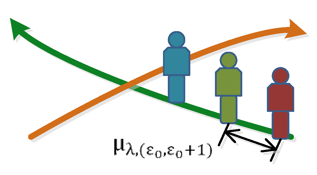
The minimum display frame interval number μ is an interactive definition parameter. Subgraphs I((λ,ε0),j), I((λ,ε0 + 1),j) are displayed in the virtual scene when the value of μ is determined, and the actual frame interval number between two moving object subgraphs in the same trajectory, which is denoted as μ(λ, (ε0,ε0 + 1)) (Figure 6), is calculated as follows:
where υε denotes the number of subgraphs for the εth moving object, and υ(ε + 1) denotes the number of frame subgraphs for the (ε + 1)th moving object.
μ(λ,(ε0,ε0 + 1)) = Max(υε − υ(ε + 1) + μ,μ),
4. Experimental Results
Through the programming experiment, the visualization effect and the timing compression rate of the surveillance video synopsis in GIS were analyzed. The sources of experimental data are as follows: the virtual geographic scene model was constructed by combining real-world images captured with manual 3D modeling while determining the camera position and camera field of view, as shown in Figure 7. The resolution of the experimental video is 1440 × 1080, with a total of 8045 frames. The experimental results are shown in the ArcScene control for visual expression.
4.1. Clustering of Moving Object Trajectories
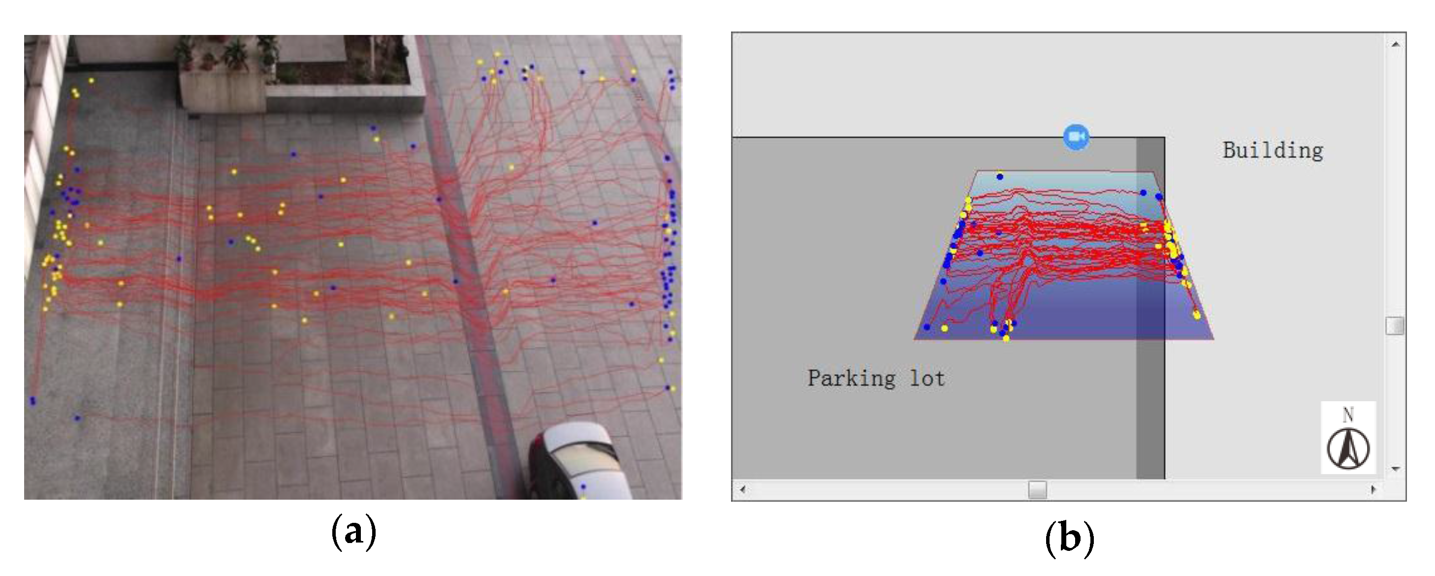
Based on the implementation of the geospatial mapping of the moving object trajectories (Figure 8), we cluster the moving target trajectories by applying the QT clustering algorithm. We set the clustering radius threshold of the trajectory entry/exit as αthr = 22.5°. Trajectories with the same entry and exit clustering number are clustered with similar trajectories, as shown in Figure 9 (yellow points represent entries, blue points represent exits). From the results of trajectory clustering, clusters calculated from the QT algorithm have a clear geographic direction. For example, cluster number one represents a set of moving objects moving from west to east, cluster number two represents a set of moving objects moving from southwest to east, cluster number three represents a set of moving objects moving from east to west, and cluster number four represents a set of moving objects moving from the east to southwest. The trajectory clustering extracts moving object trajectories with similar geographic direction, which is beneficial to the discrimination of moving objects in the video synopsis process.
4.2. Visualization of Surveillance Video Synopsis in GIS
For each trajectory cluster, we separately search for the centerline and display it in the virtual geographic scene, along with its corresponding moving object subgraphs, as shown in Figure 10. In the case of the minimum display frame interval number μ = 20, the synchronization parameters ODSR and CDSR values, as well as the corresponding video synopsis results, are obtained (Figure 11). Figure 11a shows the movement of the moving objects from east to west in the geographic space, and Figure 11b shows the moving objects in the geographic space. Figure 11c shows the moving objects in different directions individually displayed in accordance with their trajectory cluster. Figure 11d shows the moving objects in different directions, which are displayed in accordance with their trajectory cluster. Furthermore, when ODSR = 1 and CDSR = 0, the video synopsis result is obtained by taking different values of the minimum number of interval frames (Figure 12).
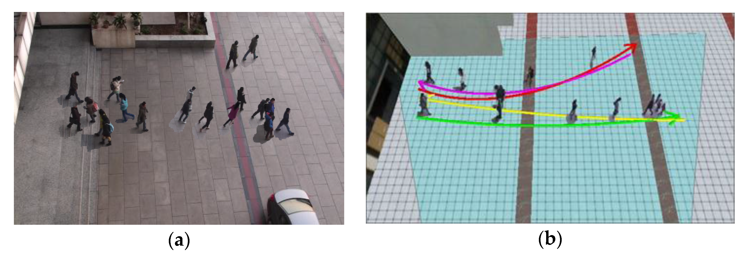
The visualization results between our approach and the image spatial video synopsis without trajectory clustering (Figure 13a) are compared to illustrate the superiority of our approach (Figure 13b). In comparison with the original approaches, video synopsis in GIS has the following advantages:
- (1)
- On the basis of georeferencing, the moving objects can be classified according to their geographical directions of the trajectory, which cannot be accurately carried out in image space.
- (2)
- There are definite display intervals and timing structural relationship between the moving objects, which avoids the crowding of the video moving objects.
- (3)
- Objects’ moving trajectories can be directly viewed and analyzed along with other geospatial targets in the geographic scene.
4.3. Evaluation of the Timing Compression Rate
In comparison to the original video, video synopsis has reduced playback time, which can be evaluated by comparing the ratio frequency between the frame number of moving object subgraphs and the original video frames. The specific evaluated content is divided into two levels: one analyzes each factor with reduction effects, and the second compares the different types of factors in different modes of expression with reduction effects. The specific method is as follows:
The frame number of the original video is marked as Nori, the expressing frame number of each subgraph is N(λ,ε) (λ = 1, 2, …, κ), and the two temporary nearby objects in the same trajectory cluster have the frame interval as μ(λ,(ε,ε + 1)) (ε = 0, …, ρ). Based on the preceding description provided, λ is the serial number of the trajectory, ε is the serial number of a moving object, κ is the number of the trajectory clusters, and ρ is the number of moving objects in the current cluster. By comparing the frame compression ratio in different moving object subgraph display modes, the length reduction performance is analyzed by using CDSR and ODSR. By comparing multiple μ values, the constrained frame compression ratio of the video for different moving object subgraph display modes, as well as the minimum number of intervals performed during the video synopsis, are analyzed.
From Table 2, when ODSR = 0, the moving objects of each trajectory cluster are separately displayed in the virtual scene. Under this circumstance, parameter μ is meaningless; hence, examining the video frame compression rate in two cases (CDSR = 0 and CDSR = 1) is necessary. When ODSR = 1, all the clusters are independently and simultaneously expressed in the virtual scene. At this point, the video frame compression rate should be calculated under different values of μ. The results are shown in Table 3.
Table 3 shows that the surveillance video synopsis in GIS significantly reduces display frame duration. Specifically, regardless of the value and μ, the frame compression ratio of is always higher than the rate of . Regardless of how the value of is taken, the frame compression rate of video synopsis always increases with the decrease of μ.
4.4. Evaluation of the Accuracy of Moving Object Retrieval
Video synopsis extracts moving objects from the original video and displays them in another form. Determining whether the moving objects in the video synopsis are similar to the objects from the original video is necessary. In this section, we quantitatively analyze this problem by proposing two characteristics, namely, the recall rate on trajectories and the match accuracy between the trajectory and the trajectory cluster. In our experiment, four trajectory clusters and 65 trajectories are extracted from the original video.
The recall rate on trajectories is put forward to check whether all the original trajectories have been assigned to the trajectory clusters in the process of trajectory clustering as follows:
where Nclu denotes the number of trajectories in all trajectory clusters and Nori denotes the number of trajectories extracted from the original video. After substituting the corresponding data, we obtain η = 98.5%, which is acceptable.
η = Nclu/Nori,
The match accuracy between the trajectory and the trajectory cluster is put forward to determine whether each of the original trajectories has been precisely assigned to the appropriate trajectory cluster. By traversing the set of all original trajectories and trajectory clusters, the match accuracy on each pair of trajectory and trajectory cluster is calculated. The calculation includes the following three steps: (1) construction of the trajectory cluster fitting boundary, (2) coincidence calculation between the trajectory and the trajectory cluster, and (3) determination of the match accuracy situation.
The construction of the trajectory cluster fitting boundary is carried out as follows. For a trajectory cluster Cλ, its fitting boundary line PL(λ,side) is defined as follows:
where side denotes the left/right direction of the trajectory cluster, t(λ,side,start) denotes the start point of the fitting boundary line, t(λ,side,end) denotes the end point of the fitting boundary line, cof(λ,side) denotes the polynomial coefficients of the fitting boundary line, and σ(λ,i) refers to the polynomial coefficients in different orders. The left/right scatter curves T(λ,left)/T(λ,right) of the trajectory cluster Cλ are calculated using the boundary line offset method for all trajectories in the trajectory cluster Cλ (as shown in Figure 14) to obtain these parameters. Then, the polynomial coefficients of the fitting boundary line are calculated on the scatter curve.
PL(λ,side) = {t(λ,side,start), t(λ,side,end), cof(λ,side)} (side = {left,right}),
cof(λ,side) = {σ(λ,i) (i = 1, …, Ο)},
The coincidence calculation between the trajectory and the trajectory cluster is carried out as follows: The fitting line of trajectory L is calculated and the polynomial coefficients are obtained as follows:
where σ(L,i) refers to the polynomial coefficients in different orders. Then, the abstract distance between the fitting trajectory line and the fitting boundary line is calculated as follows:
cofL = {σ(L,i) (i = 0, 1, …, Ο)},
If the following conditions are satisfied, then trajectory L and trajectory cluster Cλ are considered to be matched:
where β is a pre-specified threshold, and cof(λ,side) could be either left or right.
dis(cof(λ,side),cofL)/dis(cof(λ,left),cof(λ,right)) ≤ β (β < 1, side = {left,right}),
For each pair of trajectory and trajectory cluster, three types of situations could highlight match accuracy: “true positive,” “true negative,” and “false positive.” “True positive” means that the trajectory positively belongs to this trajectory cluster and that it has been assigned to this trajectory cluster. “True negative” indicates that the trajectory negatively belongs to this trajectory cluster but that it has been assigned to this trajectory cluster. “False positive” means that the trajectory positively belongs to this trajectory cluster but that it has not been assigned to this trajectory cluster. As previously illustrated, “True Positive” is the correct match situation, whereas “True negative” and “false positive” are the incorrect match situations. When the value of β is extremely small, determining match accuracy is difficult. In this experiment, β is valued starting from 0.7 and is increased by the step length of 0.05 (as shown in Table 4).
The experimental results show that regardless of the value of parameter β in the evaluation model, the ratio of “true negative” and “false positive” is sufficiently low in the clustering process of this method. The ratio of the “true positive” type is higher than 95%. The experimental results show the effectiveness of our method in classifying moving objects into different trajectory clusters and the credibility of the classification indexing and expression of moving objects in video synopsis.
5. Conclusions and Discussion
An approach called surveillance video synopsis in GIS is constructed in this paper. This approach comprehensively analyzes and integrates the expression between video and geospatial information while simultaneously improving video browsing efficiency. Based on the results of video moving object extraction and geospatial position, we constructed a moving object storage model, applied a virtual geographic scene as the background of video synopsis, and used the fusion expression mode on the geographical scene and moving object subgraphs. The moving object trajectories are clustered based on their geospatial directions to create a video synopsis. Our approach can sequentially and efficiently express video moving objects and integrate dynamic video information with geospatial information in GIS, thereby considerably reducing the display time. The main contributions of this work are as follows:
- (1)
- This study proposed an approach for video synopsis in GIS by extensively applying the model to the integration of video moving objects and GIS.
- (2)
- The proposed approach improves video browsing efficiency while integrating the expression of video and geospatial information.
- (3)
- This work describes the general process and technical details of video synopsis in GIS, discusses the characteristics of the moving object expression model, and evaluates the timing compression rate and moving object retrieval accuracy in the realization of video synopsis.
Notably, our method for video synopsis could only be applied to geographical scenes where crowd movements are dispersed. For geographical scenes with intensive pedestrian movement flow, our video synopsis method is not suitable for browsing videos in a short time. In the future, we will attempt to analyze geospatial video flow, traffic, and other sports streams. We will also attempt to jointly utilize mobile location cameras, multi-camera surveillance networks, and other related constraints in the field of video synopsis.
Acknowledgments
The work described in this paper was supported by the National Natural Science Foundation of China (NSFC) (grant nos. 41401442, 41771420, 41401436), the National High Technology Research and Development Program of China (grant no. 2015AA123901), the National Key Research and Development Program (grant no. 2016YFE0131600), the Sustainable Construction of Advantageous Subjects in Jiangsu Province (grant no. 164320H116), and the Priority Academic Program Development of Jiangsu Higher Education Institutions.
Author Contributions
Yujia Xie was principal to all phases of the investigation, including the giving of advice on the literature review, analysis, designing the approach, performing the experiments. Xuejue Liu and Meizhen Wang conceived the idea for the project, and supervised and coordinated the research activity. Yiguang Wu helped to support the experimental datasets and analyzed the data. All authors participated in the editing of the paper.
Conflicts of Interest
The authors declare no conflicts of interest.
References
- Pritch, Y.; Rav-Acha, A.; Peleg, S. Non-chronological video synopsis and indexing. IEEE Trans. Pattern Anal. Mach. Intell. 2008, 30, 1971–1984. [Google Scholar] [CrossRef] [PubMed]
- Sobral, A.; Vacavant, A. A comprehensive review of background subtraction algorithms evaluated with synthetic and real videos. Comput. Vis. Image Underst. 2014, 122, 4–21. [Google Scholar] [CrossRef]
- Bouwmans, T. Traditional and recent approaches in background modeling for foreground detection: An overview. Comput. Sci. Rev. 2014, 11, 31–66. [Google Scholar] [CrossRef]
- Cheng, Y.C.; Lin, K.Y.; Chen, Y.S.; Tarng, J.H.; Yuan, C.Y.; Kao, C.Y. Accurate planar image registration for an integrated video surveillance system. In Proceedings of the CIVI’09 IEEE Workshop on Computational Intelligence for Visual Intelligence, Nashville, TN, USA, 30 March–2 April 2009; pp. 37–43. [Google Scholar]
- Wu, C.; Zhu, Q.; Zhang, Y.T.; Du, Z.Q.; Zhou, Y.; Xie, X.; He, F. An Adaptive Organization Method of Geovideo Data for Spatio-Temporal Association Analysis. ISPRS Ann. Photogramm. Remote Sens. Spat. Inf. Sci. 2015, 2, 29–34. [Google Scholar] [CrossRef]
- Puletic, D. Generating and Visualizing Summarizations of Surveillance Videos; George Mason University: Fairfax, VA, USA, 2012. [Google Scholar]
- Gallo, N.; Thornton, J. Fast dynamic video content exploration. In Proceedings of the IEEE International Conference on Technologies for Homeland Security (HST), Waltham, MA, USA, 12–14 November 2013; pp. 271–277. [Google Scholar]
- Park, Y.; An, S.; Chang, U.; Kim, S. Region of Interest Based Video Synopsis. U.S. Patent 9,269,245, 23 February 2016. [Google Scholar]
- Lewis, J.; Grindstaff, G.; Whitaker, S. Open Geospatial Consortium Geo-Video Web Services; Open Geospatial Consortium: Wayland, MA, USA, 2006; pp. 1–36. [Google Scholar]
- Ma, Y.; Zhao, G.; He, B. Design and implementation of a fused system with 3DGIS and multiple-video. Comput. Appl. Softw. 2012, 29, 109–112. [Google Scholar]
- Takehara, T.; Nakashima, Y.; Nitta, N.; Babaguchi, N. Digital diorama: Sensing-based real-world visualization. In Proceedings of the International Conference on Information Processing and Management of Uncertainty in Knowledge-Based Systems, Dortmund, Germany, 28 June–2 July 2010; pp. 663–672. [Google Scholar]
- Roth, P.M.; Settgast, V.; Widhalm, P.; Lancelle, M.; Birchbauer, J.; Brandle, N.; Havemann, S.; Bischof, H. Next-generation 3D visualization for visual surveillance. In Proceedings of the 8th IEEE International Conference on Advanced Video and Signal-Based Surveillance (AVSS), Klagenfurt, Austria, 30 August–2 September 2011; pp. 343–348. [Google Scholar]
- Xie, Y.; Liu, X.; Wang, M.; Wu, Y. Integration of GIS and Moving Objects in Surveillance Video. ISPRS Int. Geo Inf. 2017, 6, 94. [Google Scholar] [CrossRef]
- Chen, Y.Y.; Huang, Y.H.; Cheng, Y.C.; Chen, Y.S. A 3-D surveillance system using multiple integrated cameras. In Proceedings of the IEEE International Conference on Information and Automation (ICIA), Harbin, China, 20–23 June 2010; pp. 1930–1935. [Google Scholar]
- Yang, Y.; Chang, M.C.; Tu, P.; Lyu, S. Seeing as it happens: Real time 3D video event visualization. In Proceedings of the IEEE International Conference on Image Processing (ICIP), Quebec City, QC, Canada, 27–30 September 2015; pp. 2875–2879. [Google Scholar]
- Ji, Z.; Su, Y.; Qian, R.; Ma, J. Surveillance video summarization based on moving object detection and trajectory extraction. In Proceedings of the IEEE 2nd International Conference on Signal Processing Systems (ICSPS), Dalian, China, 5–7 July 2010; Volume 2, pp. 250–253. [Google Scholar]
- Sun, L.; Ai, H.; Lao, S. The dynamic videobook: A hierarchical summarization for surveillance video. In Proceedings of the IEEE 20st International Conference on Image Processing (ICIP), Melbourne, Australia, 15–18 September 2013; pp. 3963–3966. [Google Scholar]
- Chiang, C.C.; Yang, H.F. Quick Browsing Approach for Surveillance Videos. Int. J. Comput. Technol. Appl. 2013, 4, 232–237. [Google Scholar]
- Chen, S.C.; Lin, K.; Lin, S.Y.; Chen, K.W.; Lin, C.W.; Chen, C.S.; Hung, Y.P. Target-driven video summarization in a camera network. In Proceedings of the IEEE 20st International Conference on Image Processing (ICIP), Melbourne, Australia, 15–18 September 2013; pp. 3577–3580. [Google Scholar]
- Chen, K.W.; Lee, P.J.; Hung, Y.P. Egocentric view transition for video monitoring in a distributed camera network. In Advances in Multimedia Modeling; Springer: Berlin/Heidelberg, Germany, 2011; pp. 171–181. [Google Scholar]
- Wang, Y.; Bowman, D.A. Effects of navigation design on Contextualized Video Interfaces. In Proceedings of the IEEE Symposium on 3D User Interfaces (3DUI), Singapore, 19–20 March 2011; pp. 27–34. [Google Scholar]
- Lewis, P.; Fotheringham, S.; Winstanley, A. Spatial video and GIS. Int. J. Geogr. Inf. Sci. 2011, 25, 697–716. [Google Scholar] [CrossRef]
- Wang, X. Intelligent multi-camera video surveillance: A review. Pattern Recognit. Lett. 2013, 34, 3–19. [Google Scholar] [CrossRef]
- Baklouti, M.; Chamfrault, M.; Boufarguine, M.; Guitteny, V. Virtu4D: A dynamic audio-video virtual representation for surveillance systems. In Proceedings of the IEEE 3rd International Conference on Signals, Circuits and Systems (SCS), Medenine, Tunisia, 6–8 November 2009; pp. 1–6. [Google Scholar]
- De Haan, G.; Piguillet, H.; Post, F. Spatial Navigation for Context-Aware Video Surveillance. IEEE Comput. Gr. Appl. 2010, 30, 20–31. [Google Scholar] [CrossRef] [PubMed]
- Hao, L.; Cao, J.; Li, C. Research of GrabCut algorithm for single camera video synopsis. In Proceedings of the IEEE Fourth International Conference on Intelligent Control and Information Processing (ICICIP), Beijing, China, 9–11 June 2013; pp. 632–637. [Google Scholar]
- Fu, W.; Wang, J.; Zhao, C.; Lu, H.; Ma, S. Object-centered narratives for video surveillance. In Proceedings of the 19th IEEE International Conference on Image Processing (ICIP), Orlando, FL, USA, 30 September–3 October 2012; pp. 29–32. [Google Scholar]
- Decombas, M.; Dufaux, F.; Pesquet-Popescu, B. Spatio-temporal grouping with constraint for seam carving in video summary application. In Proceedings of the IEEE 18th International Conference on Digital Signal Processing (DSP), Fira, Greece, 1–3 July 2013; pp. 1–8. [Google Scholar]
- Li, Z.; Ishwar, P.; Konrad, J. Video condensation by ribbon carving. IEEE Trans. Image Process. 2009, 18, 2572–2583. [Google Scholar] [PubMed]
- Huang, C.R.; Chen, H.C.; Chung, P.C. Online surveillance video synopsis. In Proceedings of the IEEE International Symposium on Circuits and Systems (ISCAS), Seoul, Korea, 20–23 May 2012; pp. 1843–1846. [Google Scholar]
- Chiang, C.C.; Yang, H.F. Quick browsing and retrieval for surveillance videos. Multimed. Tools Appl. 2015, 74, 2861–2877. [Google Scholar] [CrossRef]
- Wang, S.; Yang, J.; Zhao, Y.; Cai, A.; Li, S.Z. A surveillance video analysis and storage scheme for scalable synopsis browsing. In Proceedings of the IEEE International Conference on Computer Vision Workshops (ICCV Workshops), Barcelona, Spain, 6–13 November 2011; pp. 1947–1954. [Google Scholar]
- Wang, S.Z.; Wang, Z.Y.; Hu, R. Surveillance video synopsis in the compressed domain for fast video browsing. J. Vis. Commun. Image Represent. 2013, 24, 1431–1442. [Google Scholar] [CrossRef]
- Zhou, Y. Fast browser and index for large volume surveillance video. J. Comput. Appl. 2012, 32, 3185–3188. [Google Scholar] [CrossRef]
- Lu, S.P.; Zhang, S.H.; Wei, J.; Hu, S.M.; Martin, R.R. Timeline Editing of Objects in Video. IEEE Trans. Vis. Comput. Gr. 2013, 19, 1218–1227. [Google Scholar]
- Sun, L.; Xing, J.; Ai, H.; Lao, S. A tracking based fast online complete video synopsis approach. In Proceedings of the IEEE 21st International Conference on Pattern Recognition (ICPR), Tsukuba, Japan, 11–15 November 2012; pp. 1956–1959. [Google Scholar]
- Nie, Y.; Xiao, C.; Sun, H.; Li, P. Compact Video Synopsis via Global Spatiotemporal Optimization. IEEE Trans. Vis. Comput. Graphics 2013, 19, 1664–1676. [Google Scholar] [CrossRef] [PubMed]
- Huang, C.R.; Chung, P.C.J.; Yang, D.K.; Chen, H.C.; Huang, G.J. Maximum a posteriori probability estimation for online surveillance video synopsis. IEEE Trans. Circuits Syst. Video Technol. 2014, 24, 1417–1429. [Google Scholar] [CrossRef]
- Feng, S.; Lei, Z.; Yi, D.; Li, S.Z. Online content-aware video condensation. In Proceedings of the IEEE Conference on Computer Vision and Pattern Recognition (CVPR), Providence, RI, USA, 16–21 June 2012; pp. 2082–2087. [Google Scholar]
- Fu, W.; Wang, J.; Gui, L.; Lu, H.; Ma, S. Online video synopsis of structured motion. Neurocomputing 2014, 135, 155–162. [Google Scholar] [CrossRef]
- Xu, M.; Li, S.Z.; Li, B.; Yuan, X.T.; Xiang, S.M. A set theoretical method for video synopsis. In Proceedings of the 1st ACM international conference on Multimedia information retrieval, Vancouver, BC, Canada, 30–31 October 2008; pp. 366–370. [Google Scholar]
- Zhou, X.; Yang, C.; Yu, W. Moving object detection by detecting contiguous outliers in the low-rank representation. IEEE Trans. Pattern Anal. Mach. Intell. 2013, 35, 597–610. [Google Scholar] [CrossRef] [PubMed]
- Smeulders, A.; Chu, D.; Cucchiara, R.; Calderara, S.; Dehghan, A.; Shah, M. Visual tracking: An experimental survey. IEEE Trans. Pattern Anal. Mach. Intell. 2014, 36, 1442–1468. [Google Scholar] [PubMed]
- Zhang, X.; Liu, X.; Wang, S.; Yang, L. Mutual Mapping Between Surveillance Video and 2D Geospatial Data. Geomat. Inf. Sci. Wuhan Univ. 2015, 40, 1130–1136. [Google Scholar]
- Heyer, L.J.; Kruglyak, S.; Yooseph, S. Exploring Expression Data: Identification and Analysis of CoexpressedGenes. Genome Res. 1999, 9, 1106–1115. [Google Scholar] [CrossRef] [PubMed]
Figure 1.
Flowchart of key technologies of surveillance video synopsis in GIS.
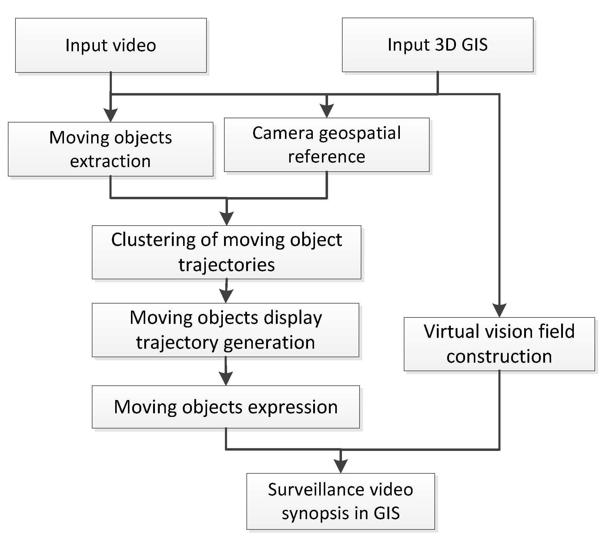
Figure 2.
Camera and geospatial coordinate system and image space coordinate system.

Figure 3.
Positional relationship between geospatial sight quadrilateral and central point and entry/exit point of the trajectories.
Figure 3.
Positional relationship between geospatial sight quadrilateral and central point and entry/exit point of the trajectories.
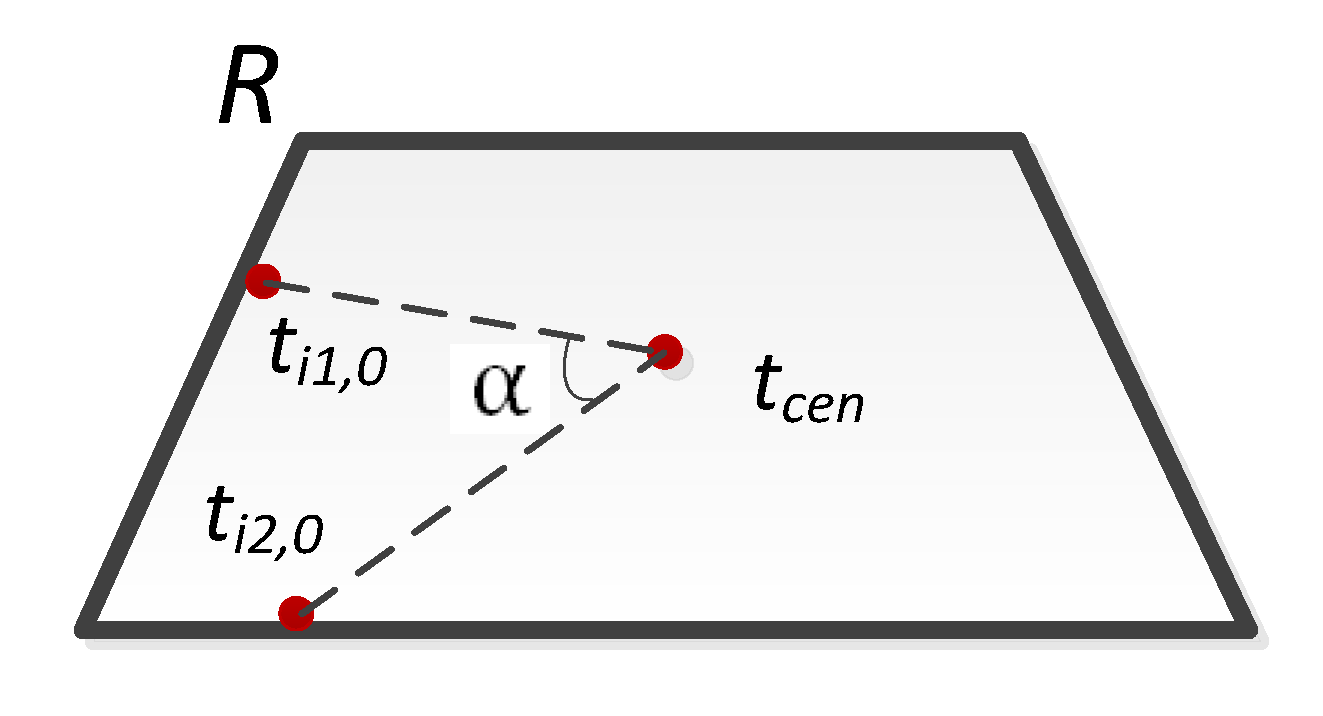
Figure 4.
Virtual scene viewpoint selection.
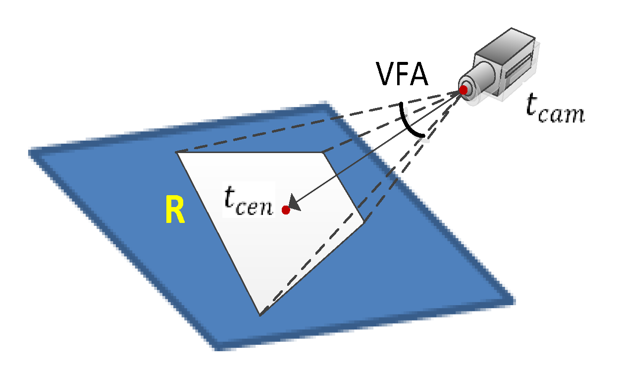
Figure 5.
Positional relationship between original scatterplot trajectories and fitting centerline.
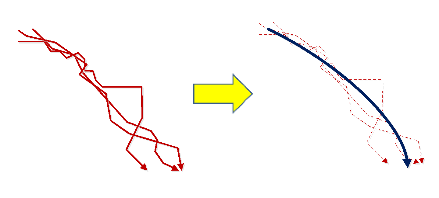
Figure 6.
Number of interval frames expression of moving objects.

Figure 7.
Background selection of video synopsis on geographic scene.
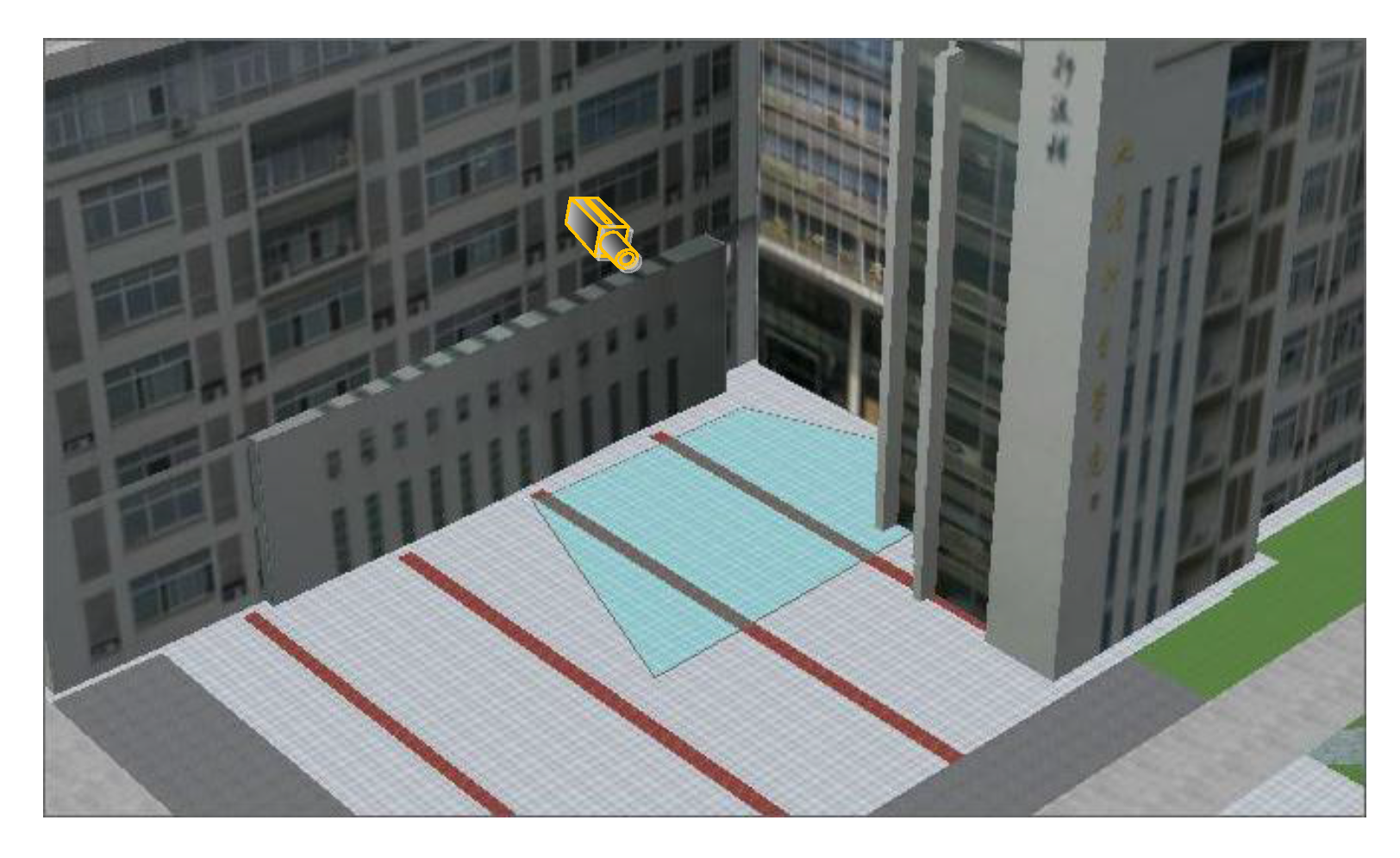
Figure 8.
Trajectories of moving objects. (a) Trajectories represented in image space; and (b) trajectories represented in geographic space.
Figure 8.
Trajectories of moving objects. (a) Trajectories represented in image space; and (b) trajectories represented in geographic space.

Figure 9.
Trajectory clustering results. (a) Cluster No. 1; (b) Cluster No. 2; (c) Cluster No. 3; and (d) Cluster No. 4.
Figure 9.
Trajectory clustering results. (a) Cluster No. 1; (b) Cluster No. 2; (c) Cluster No. 3; and (d) Cluster No. 4.
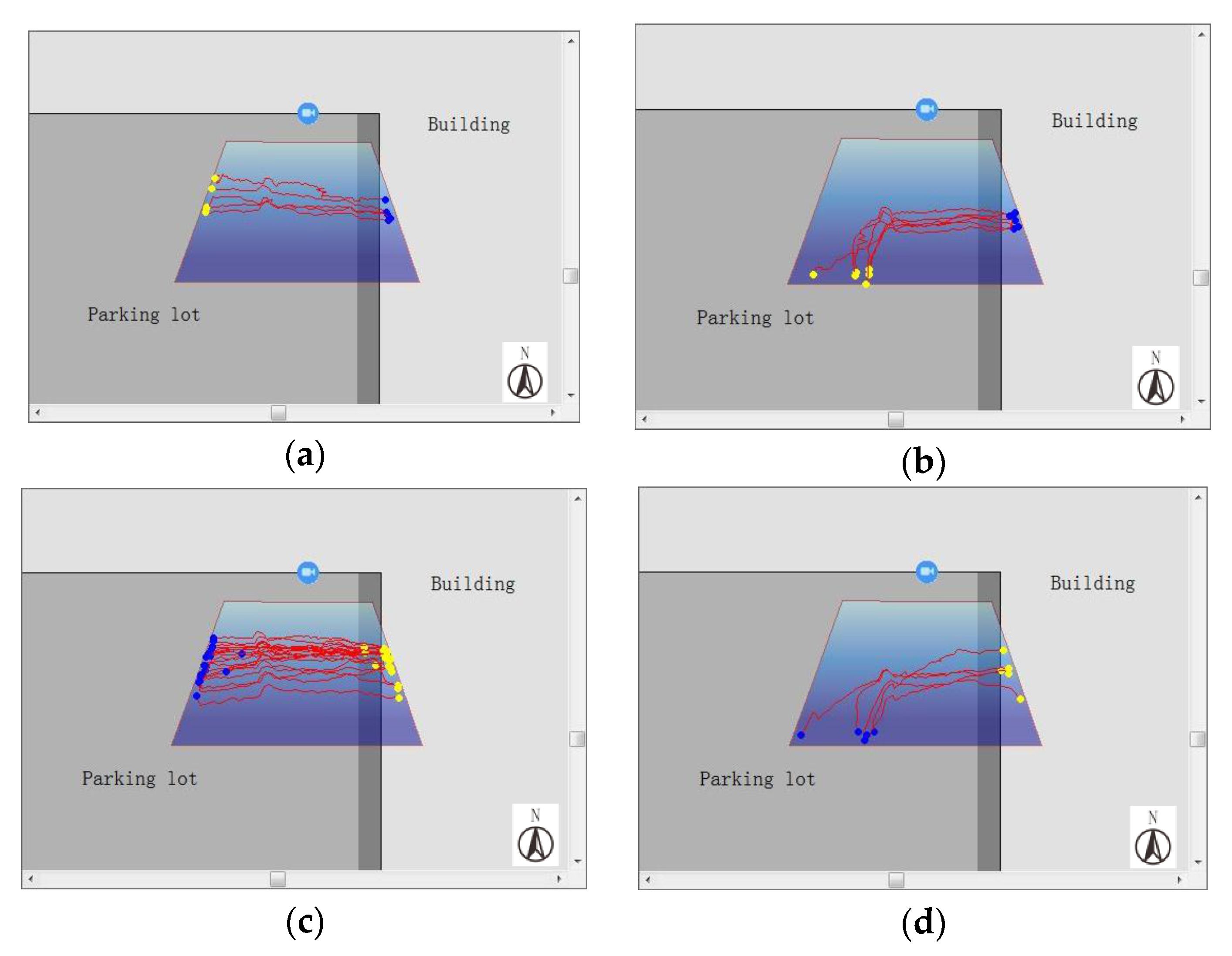
Figure 10.
Fitting central curve of trajectory clusters along with the corresponding moving object subgraphs: (a) pedestrians leaved from the building to the west; (b) pedestrians leaved from the building to the southwest; (c) pedestrians entered the building from the west; (d) pedestrians entered the building from the southwest.
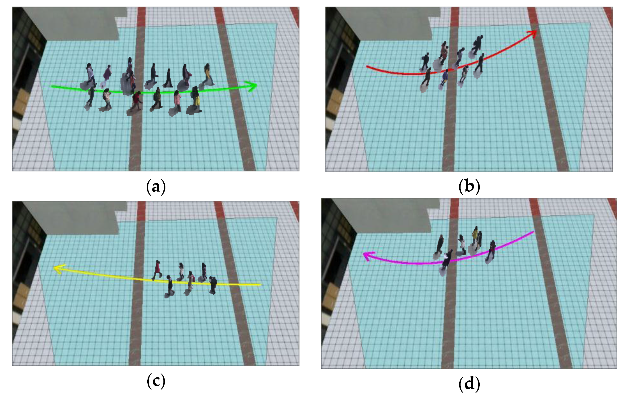
Figure 11.
Result of video synopsis in GIS (μ = 20): (a) ODSR = 0, CDSR = 0; (b) ODSR = 1, CDSR = 0; (c) ODSR = 0, CDSR = 1; and (d) ODSR = 1, CDSR = 1.
Figure 11.
Result of video synopsis in GIS (μ = 20): (a) ODSR = 0, CDSR = 0; (b) ODSR = 1, CDSR = 0; (c) ODSR = 0, CDSR = 1; and (d) ODSR = 1, CDSR = 1.
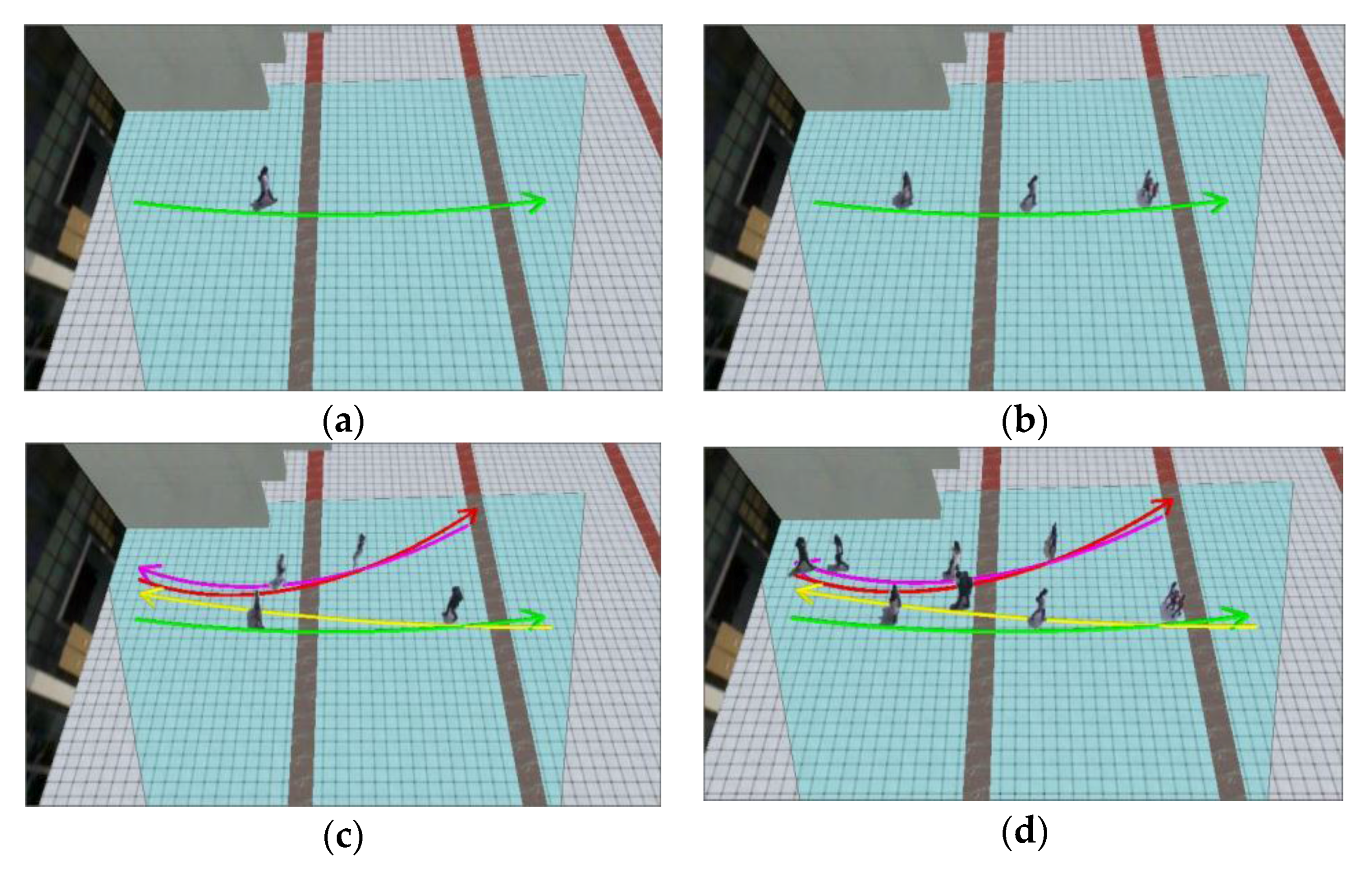
Figure 12.
Video synopsis result (ODSR = 1, CDSR = 0): (a) μ = 5; and (b) μ = 20.
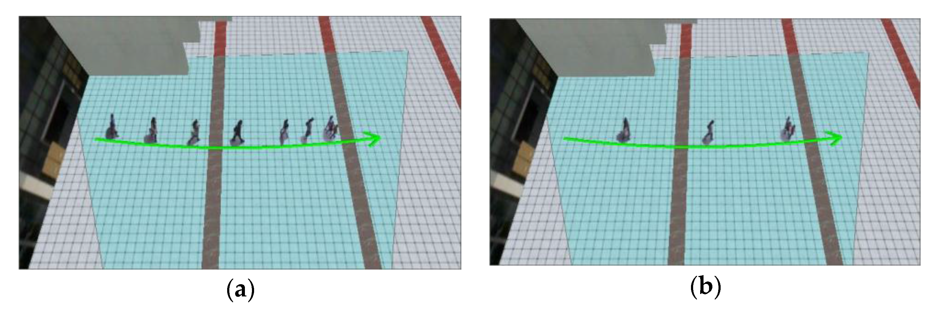
Figure 13.
Comparison of results of video synopsis on an image and on a geographic scene. (a) Video synopsis on a geographic scene; and (b) video synopsis on an image.
Figure 13.
Comparison of results of video synopsis on an image and on a geographic scene. (a) Video synopsis on a geographic scene; and (b) video synopsis on an image.

Figure 14.
Positional relationship between the original and the offset scatter curve.

Table 1.
Expression patterns of the trajectory clusters.
| ODSR | 0 | 1 | |
|---|---|---|---|
| CDSR | |||
| 0 |  |  | |
| 1 |  |  | |
Table 2.
Calculation method of frame compression rate of video synopsis.
| CDSR | ODSR = 0 | ODSR = 1 |
|---|---|---|
| 0 | ||
| 1 |
Table 3.
Calculation results of frame compression rate of video synopsis in different subgraph expression modes.
Table 3.
Calculation results of frame compression rate of video synopsis in different subgraph expression modes.
| ODSR | ODSR = 0 | ODSR = 1 = 5 | ODSR = 1 = 10 | ODSR = 1 = 20 | ODSR = 1 = 30 |
|---|---|---|---|---|---|
| 0 | 19.53% | 19.53% | 6.61% | 8.23% | 11.46% |
| 1 | 11.45% | 3.00% | 4.05% | 6.17% | 8.28% |
Table 4.
Values of every situation of match accuracy with different β.
| β | True Positive | True Negative | False Positive |
|---|---|---|---|
| 0.7 | 95.2% | 4.8% | 0 |
| 0.75 | 98.4% | 1.6% | 0 |
| 0.8 | 96.8% | 1.6% | 1.6% |
| 0.85 | 96.8% | 1.6% | 1.6% |
| 0.9 | 98.4% | 0 | 1.6% |
| 0.95 | 98.4% | 0 | 1.6% |
© 2017 by the authors. Licensee MDPI, Basel, Switzerland. This article is an open access article distributed under the terms and conditions of the Creative Commons Attribution (CC BY) license (http://creativecommons.org/licenses/by/4.0/).
Share and Cite
MDPI and ACS Style
Xie, Y.; Wang, M.; Liu, X.; Wu, Y. Surveillance Video Synopsis in GIS. ISPRS Int. J. Geo-Inf. 2017, 6, 333. https://doi.org/10.3390/ijgi6110333
AMA Style
Xie Y, Wang M, Liu X, Wu Y. Surveillance Video Synopsis in GIS. ISPRS International Journal of Geo-Information. 2017; 6(11):333. https://doi.org/10.3390/ijgi6110333
Chicago/Turabian StyleXie, Yujia, Meizhen Wang, Xuejun Liu, and Yiguang Wu. 2017. "Surveillance Video Synopsis in GIS" ISPRS International Journal of Geo-Information 6, no. 11: 333. https://doi.org/10.3390/ijgi6110333
Note that from the first issue of 2016, this journal uses article numbers instead of page numbers. See further details here.