Beyond Maximum Independent Set: An Extended Integer Programming Formulation for Point Labeling

1
Institute of Geodesy and Geoinformation, University of Bonn, 53115 Bonn, Germany
2
Institut für Informatik, Universität Würzburg, 97074 Würzburg, Germany
*
Authors to whom correspondence should be addressed.
ISPRS Int. J. Geo-Inf. 2017, 6(11), 342; https://doi.org/10.3390/ijgi6110342
Submission received: 6 September 2017
/
Revised: 20 October 2017
/
Accepted: 25 October 2017
/
Published: 6 November 2017
Abstract
:Map labeling is a classical problem of cartography that has frequently been approached by combinatorial optimization. Given a set of features in a map and for each feature a set of label candidates, a common problem is to select an independent set of labels (that is, a labeling without label–label intersections) that contains as many labels as possible and at most one label for each feature. To obtain solutions of high cartographic quality, the labels can be weighted and one can maximize the total weight (rather than the number) of the selected labels. We argue, however, that when maximizing the weight of the labeling, the influences of labels on other labels are insufficiently addressed. Furthermore, in a maximum-weight labeling, the labels tend to be densely packed and thus the map background can be occluded too much. We propose extensions of an existing model to overcome these limitations. Since even without our extensions the problem is NP-hard, we cannot hope for an efficient exact algorithm for the problem. Therefore, we present a formalization of our model as an integer linear program (ILP). This allows us to compute optimal solutions in reasonable time, which we demonstrate both for randomly generated point sets and an existing data set of cities. Moreover, a relaxation of our ILP allows for a simple and efficient heuristic, which yielded near-optimal solutions for our instances.
1. Introduction
Maps and technical drawings are usually annotated with textual or pictorial labels in order to help their users understand what they see. A natural requirement to ensure readability is that labels must not intersect. Especially in printed maps where extra information cannot be added on demand, it is reasonable to label as many features (such as cities, rivers, or countries) as possible. More generally, one may introduce a weight for every possible label to represent its priority. For example, labels occluding much important information of the map background can be associated with relatively low weights, labels of important features such as large cities with high weights. This idea leads to what we term the basic map-labeling problem: Given a set of features and, for each feature, a set of label candidates, each with a positive weight, select for each feature at most one label from the set of candidates such that (i) no two selected labels intersect and (ii) the sum of the weights of the selected labels is maximized. In this article, we focus on labeling point features, though labeling line features [1] or area features [2] is equally important. In a conference paper preceding this article, we have sketched our general ideas and presented first experiments [3].
When labeling points, a label candidate is usually a rectangle that contains the name of a feature and that is placed close to the corresponding point. In algorithmic terms, an optimal solution to the basic map-labeling problem is a maximum-weight independent subset of the given set of label candidates, where a set of labels is independent if it does not contain two intersecting labels. Additionally, if a point can have multiple non-intersecting label candidates, one has to require at most one label for each point.
For the above basic problem, highly sophisticated optimization methods have been developed, ranging from exact approaches based on mathematical programming [4], via approximation algorithms [5], to specialized heuristics [6]. We argue, however, that the basic map-labeling problem lacks expressiveness. In particular, to judge whether placing a label leads to ambiguous label–point associations, it is important to know which other labels are placed. Generally, a label candidate can be more or less favorable depending on which other label candidates are selected in its surroundings. Such influences are not modeled in the basic problem.
Furthermore, an optimal solution to the basic problem always has the property that no label can be added to it (without intersecting other labels). This means that optimal solutions tend to be densely packed and, thus, the resulting map can be rather illegible, even though no two labels intersect each other. For example, in his fundamental work, Bertin [7] suggested that the graphic density should not exceed ten symbols per cm. Such a requirement cannot be ensured by defining the weights of the symbols (in our case labels). Our new method, however, can handle it.
Kern and Brewer [8] and, more recently, Rylov and Reimer [9] have provided overviews of criteria that have been considered in the cartographic literature on map labeling. Thereby, Rylov and Reimer have developed what they call a “comprehensive multi-criteria model” for point labeling, which also deals with graphical clutter and ambiguous label–point associations. They have computed solutions with popular meta heuristics (a greedy algorithm, discrete gradient descent, and simulated annealing), which often yield solutions of high quality but do not guarantee an optimal solution. An exact method for a similarly comprehensive model, however, has not been developed yet.
To close the gap between sophisticated algorithmic techniques for the basic labeling problem and more comprehensive cartographic models for labeling, we focus on the development of an exact method for an extension of the basic labeling problem, in which graphical clutter and ambiguous label–point associations are considered. Developing such a method is challenging since computing a maximum independent subset of a set of rectangles is NP-hard [10], which means that it is very unlikely that an exact algorithm with a polynomial worst-case running time for the basic map-labeling problem (or for any generalization of it) exists. On the other hand, for some classes of NP-hard problems, mathematical solvers exist that often yield optimal solutions in reasonable time. Hence, we choose an approach that takes advantages of mathematical solvers, but we are well aware of the following general disadvantage of such an approach:
- The running time of an exact method for an NP-hard problem can be high and difficult to predict.
On the other hand, an exact method has multiple advantages:
- The quality of a solution obtained with a heuristic can be arbitrarily far away from optimum and difficult to predict.
- With our exact method, we directly profit from every algorithmic speedup that is introduced to mathematical solvers for the class of problems to which our problem belongs. Such improvements are being made constantly [11].
- Often, an exact method can be transformed into a faster inexact (that is, heuristic) method, without much engineering effort. Though the development of a heuristic is not our primary goal, we will present such a transformation for our method.
- Even though an exact method can be too slow, for example, for real-time applications, the optimal solutions obtained with it can be used as benchmarks to assess the quality of faster heuristics.
Due to the latter reason, heuristic and exact approaches can complement each other, meaning that we do not aim to replace the state-of-the-art heuristic methods for point labeling with our method but to add a useful method to an existing toolbox.
Our exact method is based on a formalization of the point-feature labeling problem as an integer linear program (ILP), which generally consists of a linear objective function and a set of linear inequality constraints, both of which are defined over a set of integer variables that encode a solution to the problem [12]. Often, the integer variables are restricted to values 0 and 1, in which case they are termed decision variables or 0–1 variables. For example, one may ask to find such that the constraints and are satisfied and the objective is minimized. By testing all variable assignments, it is easy to see that this ILP has an optimal solution of objective value 2 for . However, explicitly enumerating all possible solutions is prohibitive already for a relatively small number n of variables. Therefore, ILP solvers (for example, Gurobi or CPLEX) use much more sophisticated solution strategies such as branch and cut. Though solving an ILP is generally NP-hard, the existing problem solvers often yield optimal solutions for realistic-size problem instances in reasonable time. Therefore, we consider integer linear programming as a promising approach.
Before we summarize our contribution, we note that Rylov and Reimer [9] expressed their model in a form that is similar to an ILP but does not satisfy the definition of an ILP. In fact, they do not use the term integer (linear) program but the much more general term combinatorial optimization problem, which correctly describes their model. The authors’ model contains 0–1 variables to encode whether a label candidate i is selected as the label for a point feature j (in which case ) or not (). Each variable appears with a coefficient in the objective function and the aim is to maximize the sum of over all i and j. The model does not meet the definition of an ILP, however, since for computing the coefficient as defined by the authors one has to know which other label candidates are selected in a certain neighborhood of the label candidate i. For example, is influenced by a term that measures graphical clutter and “reflects proximity of placed labels to each other”—such a dependency between the solution (that is, the placed labels) and the coefficients of the variables is not allowed in an ILP and cannot be handled by existing ILP solvers. On the other hand, if one neglects some quality criteria of the authors’ model, the coefficients of the variables depend only on the input. Then, one obtains an ILP, but only for the basic map-labeling problem that we stated above. An interesting open question is how point-feature labeling can be modeled as an ILP if criteria involving geometric constellations of multiple labels have to be taken into account, for example, avoiding a high graphical density (clutter) or ambiguous label–point associations.
Our contribution is as follows. We present an ILP for point labeling that allows its users to control the graphic density of the output map and to penalize constellations of labels and points in which the label–feature associations are ambiguous. Our ILP extends an ILP for the basic map-labeling problem, which already forbids intersections of labels and allows for the consideration of all criteria that can be expressed as a weighted sum of 0–1 variables encoding the selection of label candidates. For example, we can increase the weights of variables for labels of important point features or decrease the weights of variables for labels at unfavorable positions. We require a discrete set of label candidates as input, but we do not make restricting assumptions with respect to how the label candidates are generated. Our model is thus flexible enough, for example, to deal with the popular four-position model or eight-position model [13], in which four or eight label candidates are constructed for each point feature; see Figure 1.
We suggest using exact algorithms implemented in ILP solvers (such as CPLEX or Gurobi) to compute optimal solutions to our model, but we also introduce a rounding heuristic to achieve a better running time. Furthermore, we discuss how to strengthen our ILP formulation in such a way that the rounding heuristic yields better solutions.
We present tests of our methods with randomly generated point sets and an existing data set of cities. In our tests, we focus on the running time of our methods, the quality of the rounding heuristic in comparison to the exact method, and the effectiveness of our model extensions concerning the graphic density and ambiguous label–point associations. On the other hand, we use very simple settings for constructing the set of label candidates and for defining the weights of the corresponding variables.
2. Related Work
First attempts to formalize the rules that govern the labeling of a map have been made by Imhof [14] and Alinhac [15]. First, cartographers [13], but later also computer scientists tried to automate the tedious process of labeling maps using heuristics, rule-based or expert systems [16]. Theoreticians focused on apparently simple special cases such as the point-feature label placement problem with four axis-aligned rectangular label candidates per point, the so-called four-position model (see Figure 1, left). Formann and Wagner [10] showed that deciding whether all points in a given instance can be labeled is NP-hard and gave approximation algorithms, which guarantee that a solution “weighs” at least a certain fraction of an (unknown) conflict-free solution of maximum weight. Around the same time, researchers such as Zoraster [4,17] started using integer linear programming for map labeling. Zoraster’s early ILP formulations were later refined by Verweij and Aardal [18]. In order to speed up the computation of optimal or near-optimal solutions, they suggested to employ so-called cutting plane techniques. Ribeiro et al. [6] presented a heuristic approach based on a relaxation of an ILP for the basic map-labeling problem. Other heuristic approaches to finding a feasible labeling of maximum total weight were based on simulated annealing [19] or used a small set of rules [20]. While most algorithms require a discrete set of candidate labels as input, the model of Van Kreveld et al. [21] allows the labels to slide, meaning that any label position is allowed where a label touches the corresponding point. Based on this model, Van Kreveld et al. [21] and Strijk and Van Kreveld [22] presented approximation algorithms for selecting a maximum independent set of labels. Meng et al. [23] and Wu et al. [24] used a model that allows a label to be placed some distance away from the corresponding point. In this model, the association between a point and its label is clarified by connecting them with a guiding line.
Been et al. [25] considered the case that a user changes the scale of the map by zooming in or out and, at any time, a conflict-free set of labels has to be presented. In this scenario, it is undesirable that labels flicker on and off, thus every label is allowed to be visible only in a single continuous range of scales, which is termed the label’s active range. Subject to this constraint and the requirement that selected labels never intersect, the authors presented approximation algorithms for maximizing the total length of all active ranges.
Several researchers considered labeling problems in which all points have to be labeled. Raidl [26] presented a heuristic approach to the problem of labeling all points such that overlaps are minimized and preferred label position are considered. Ribeiro and Lorena [27] gave two ILP formulations and ILP-based heuristics for a similar problem. Yamamoto and Lorena [28] and Alvim and Taillard [29] approached the problem using heuristic methods. Bae et al. [30] suggested charging different costs for label–label conflicts and label–point conflicts and presented a heuristic method. Gomes et al. [31,32] presented an ILP-based method and a heuristic method, respectively, for a problem in which the aim is to disperse conflicting labels as much as possible, meaning that the minimum distance between the reference points of two conflicting labels is maximized. Mauri et al. [33] developed ILP-based heuristics for the problem of labeling all points while maximizing a function that reflects both the sum of label-dependent profits and the total number of conflict-free labels. Also aiming to maximize the number of conflict-free labels, Rabello et al. [34] presented a heuristic method. We argue, however, that certain conflicts in a map must not be tolerated. In particular, a label occluding a second label is not acceptable. Therefore, we will develop our new model by extending the basic map-labeling problem, which asks to find a conflict-free labeling of maximum weight and, thus, allows some points to be left unlabeled.
Integer programming has also been applied to problems of cartography other than map labeling. For the aggregation of areas in map generalization, we [35] developed an ILP-based method and presented a comparison with an approach based on simulated annealing. Since the exact ILP-based method could not solve large problem instances, it was combined with a heuristic decomposition technique. This yielded clearly better solutions than simulated annealing for small and medium-size instances. For large instances, the two methods yielded results of similar quality.
3. Methodology
We start by recalling an ILP for the basic map-label problem, which was also used by Ribeiro et al. [6]. This ILP forms the basis for our extensions with respect to additional cartographic criteria (see Section 3.3, Section 3.4 and Section 3.5). Then, we introduce a heuristic to solve our model efficiently (see Section 3.6).
3.1. A Basic Integer Linear Program
In the basic map-labeling problem, we are given a set of features and, for each feature , a set of label candidates. The set of all label candidates is . The ILP contains a 0–1 variable for each label candidate:
Since we will later add another group of variables, we refer to the above variables as x-variables. Generally, if a variable is set to 1, the label candidate ℓ is selected; it becomes a label (For simplicity, in the sequel, by “labels” we will also mean label candidates.). Using these variables, the objective of the basic map-labeling problem is defined as follows:
where is the weight of label ℓ. The selection of intersecting labels is avoided by requiring
If the given labeling instance is such that any two label candidates of the same feature intersect, then Constraint (3) automatically ensures that any feature receives at most one label. If, however, a feature has label candidates that do not intersect each other, the following constraint needs to be added:
This ILP forms the basis for our extended model, which is why we term it the basic ILP. It has integer variables and constraints since we have to instantiate Constraint (3) at most once for each pair of label candidates.
3.2. Discussion of the Basic ILP
From a cartographic perspective, maximizing the total weight of a labeling can be reasonable since the weight of a label candidate can be defined as a function of multiple parameters. More precisely, the following criteria of the model of [9] can be modeled with label weights that depend only on the input:
- (C1)
- priorities of features,
- (C2)
- priorities of label positions,
- (C3)
- overlapping of labels or symbols for the corresponding features with other map features,
- (C4)
- percentage of water under a label for a point representing a coastal place.
An extension of the ILP for the basic map-labeling problem is necessary, however, to address the following two criteria of the model of [9]:
- (C5)
- magnitude of ambiguity between neighboring point features and their names,
- (C6)
- proximity of placed labels, which can lead to clutter.
To judge whether the association between a point label ℓ and its corresponding point p is unambiguous (see criterion (C5)), it is important to know which other points are labeled. This particularly holds if the rule is to display only those points that receive a label: With that rule, only if a point is labeled, a label ℓ can be misinterpreted as the label for . We could rule out ambiguous label–point associations by setting up hard constraints similar to Constraint (3), for example, to express that a label ℓ must never be placed together with a label for . Since such a constraint could be too strict, however, we suggest considering the clarity of associations in the objective function. This is not possible with a weighted sum of the x-variables.
A solution of the basic ILP can be cluttered and thus poor according to criterion (C6) since, among two feasible solutions and with , the solution containing more labels is always preferred. In other words, if a label can be added to a solution, then this solution cannot be optimal. Consequently, an optimal labeling tends to be densely packed with labels and may occlude the map background almost completely. In fact, in the optimization community, map labeling is referred to as a packing problem [10]. It is clearly not the objective of map labeling, however, to occlude the map background as much as possible.
Before we turn to an extension of the basic ILP, we need to admit that it is not as bad as it may seem.
First of all, every subset of an optimal solution to the basic ILP is a feasible solution. Therefore, it can be reasonable to first compute an optimal (or a close-to-optimal) solution to the basic ILP, to store this solution, and, at any time, to display only a selection of labels from S such that the map background is not occluded too much. This two-step approach of first computing a densely packed solution S without label–label intersections and then filtering S to obtain the actual labeling is particularly useful for real-time cartography. To compute a labeling in real time, the supposedly difficult part of the labeling problem—avoiding label–label intersections without losing too much information—arguably should be solved in a pre-processing step [36].
A second argument for the basic ILP is that the occlusion of the map background can be controlled by defining the labels larger than necessary. For example, the label holding a certain text can be defined by buffering the text’s bounding box with a certain distance . This in essence means that between any two displayed texts a minimum distance of is ensured. We argue that strictly requiring a minimum distance between two texts is important to ensure the legibility of each label. To avoid that large parts of the map are covered with labels, however, would have to be set to a relatively large value. This would have the undesirable effect that two points that are relatively close to each other are never labeled at the same time.
3.3. Penalizing Ambiguous Label–Feature Associations
In this section, we present an extension of the basic ILP to reduce the risk that a user interprets a label of some feature f as the label of a different feature . We first discuss this in a general context and then exemplify it for point-feature label placement.
Our model is based on a graph that contains a node for each label in L. Just as any graph, G models relationships between entities, in our case geometrical interferences between labels. Therefore, we term G the interference graph. The set E contains an edge between two labels a and b if placing both a and b is possible yet undesirable. Consequently, we term such an edge an interference.
To express how undesirable it is to place both a and b, we define a cost function . If for an edge both labels are selected at the same time, we charge the cost , meaning that the objective value is reduced by . For ease of notation, we write for with . To formalize the idea in linear terms, we introduce continuous variables
which we term y-variables. These are linked with the x-variables such that if both and for :
If at least one of the two labels is not selected, however, Constraint (6) does not have any influence on the variable . In this case, will receive the smallest possible value since, in the objective function, we will charge a cost that is proportional to . This ensures that will always receive the value 0 or 1, even though we defined as a continuous variable.
We conclude that our extended model does not need additional integer variables, which has computational advantages. Since our model has both integer variables and continuous variables, it is in fact a mixed integer linear program (MILP).
Finally, we complete our model by specifying the objective function as follows:
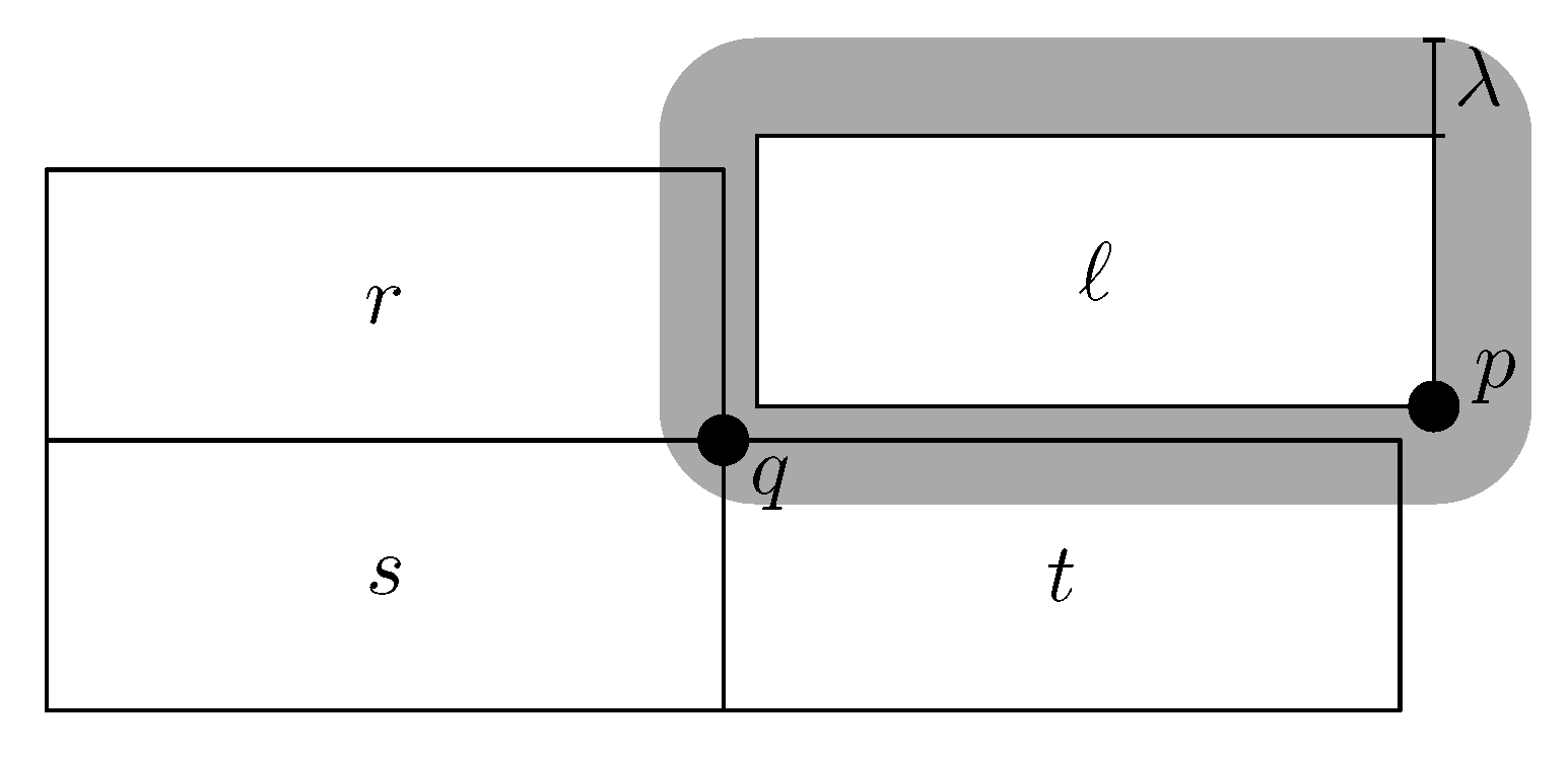
When labeling points in the four- or eight-position model, we use the following specification of the cost function c. In this case, we would like to prevent situations such as the one displayed in Figure 2. In this example, the rectangular label ℓ corresponds to the point p, yet a user may think that ℓ is the label for q, since q is within a specified distance from ℓ. Therefore, ℓ should not be displayed together with q. Assuming that q is displayed if and only if it receives a label, we can equally well say that ℓ should not be displayed together with one of the labels for q. Since the upper-right label for q is not possible in conjunction with ℓ, we add three edges to the graph G, namely , , and .
For edges and , we define the costs , where is a user-selectable parameter. For example, means that selecting ℓ with r or s is 40% less profitable than selecting ℓ without r or s. For edge , we define the cost since not only q is within distance from ℓ but also p is within distance from t. Note that , , , can be arbitrary positive numbers, which can be set to express preferences among the label candidates.
3.4. Controlling the Graphic Density of the Map
In Section 3.2, we argued that the graphic density of the map could be controlled to some degree by defining the labels larger than necessary, for example, by buffering the bounding boxes for the texts that are to be displayed. Because of Constraint (3), this in essence means that any two labels have to be separated with a certain amount of empty space between them. While Constraint (3) acts locally, we introduce a constraint that acts on a regional level to control the graphic density in an adequate way.
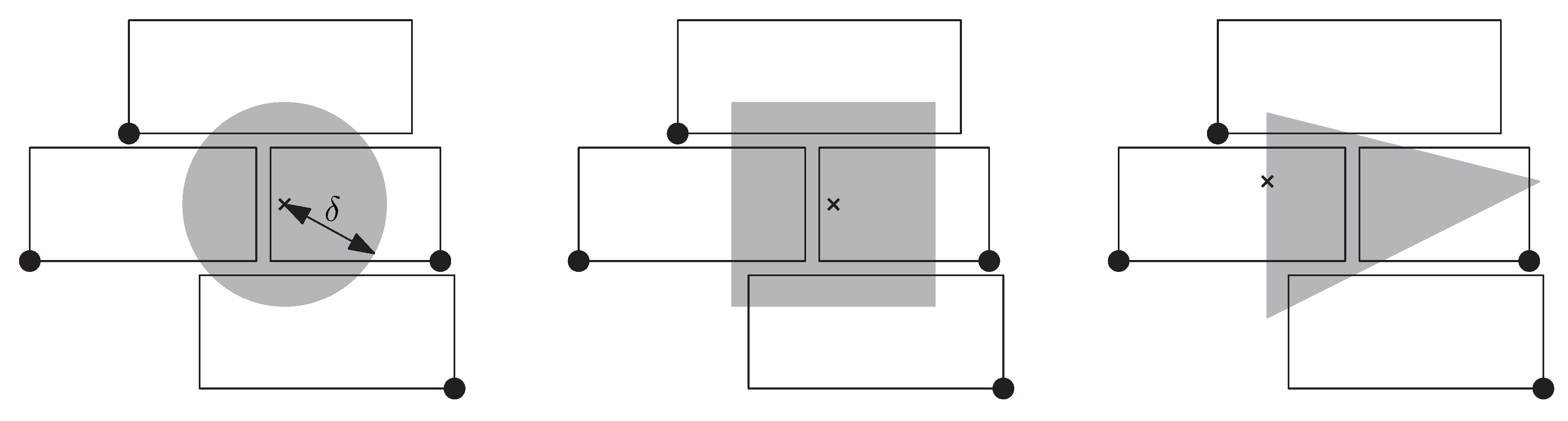
Our model relies on the definition of a region , for example, a disk of radius centered at . We require that, no matter how we translate , it never intersects more than a certain number of labels. If we define as a disk of radius , this requirement means that every disk of radius intersects at most labels; see Figure 3. We consider this requirement most promising to avoid densely packed solutions that often look like a wall of bricks, such as the one in Figure 3. To loosen up the masonry-like layout, we suggest defining slightly higher than the labels and choosing a relatively small number for , for example, 2 or 3.
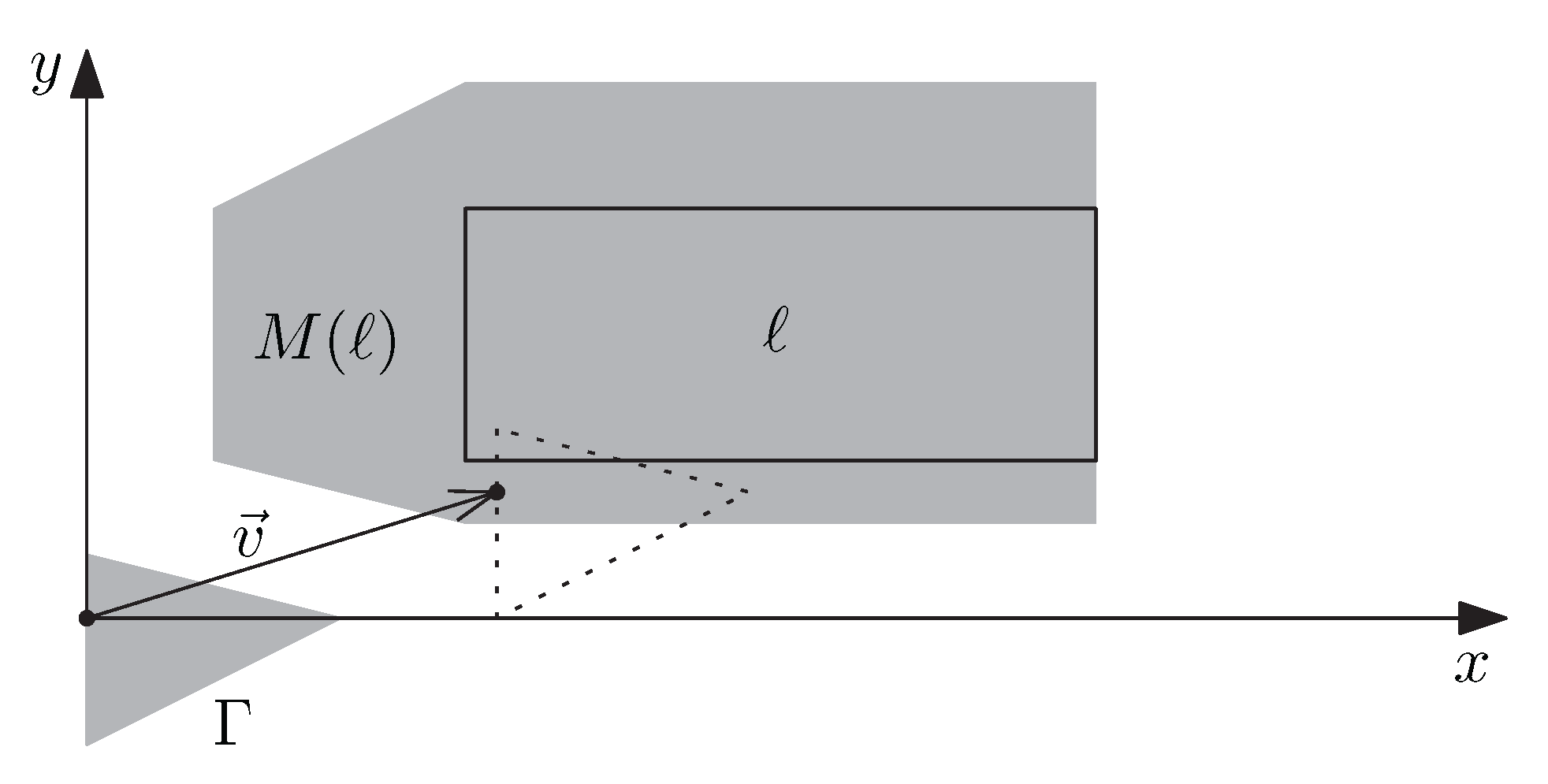
Though the number of possible translations of is infinite, we will see that our requirement can be formalized with a finite set of constraints. For this, we first introduce some notation. We denote the set of label candidates intersected by a region as . Furthermore, for each label , we define as the set of all vectors such that translating with yields a region intersecting ℓ; see Figure 4. Formally, this can be stated as
where ⊕ denotes the Minkowski sum [37]. That is, for any two sets of positions vectors,
For example, if ℓ is a rectangle and D is a disk of radius centered at the origin, then is the result of buffering ℓ with distance ; see Figure 2. Furthermore, if A is a polygon and a vector, then is the result of translating A with .
To set up the constraints of our model, we consider the arrangement formed by the boundaries of the region for each label ; see Figure 5. More formally, we consider a set of faces. For a face and any two vectors , it holds that the regions and obtained by translating with and , respectively, intersect the same labels, that is, . Hence, to ensure that, for any translation vector , intersects at most selected labels, we need only one constraint for each face of :
where is an arbitrary vector in F.
The number of instantiations of Constraint (8) equals the number of faces of . To ensure that the number of constraints is small, we require that the labels as well as the region have constant complexity, which is, for example, the case for axis-aligned rectangles (each described with four parameters) or disks (each described with three parameters). Consequently, has constant complexity, which yields that the total number of vertices and line segments of is . Since is planar, the number of faces is linear in the number of vertices, thus has faces.
We conclude that Constraint (8) requires instantiations—one for each face of —and thus (asymptotically) the extended model does not require more constraints than the basic ILP. Furthermore, our model requires the same integer variables ( for each ) as the basic ILP. On the other hand, we need additional continuous variables ( for each ), since we may need to charge a cost for each pair of labels. In practice, however, it is reasonable to assume that the graph G is sparse, since only few labels (probably a constant number of labels) will interfere with a label. Therefore, it is reasonable to assume that the number of edges of G is in and thus our ILP has the same size as the basic ILP. To set up Constraint (8), we need to compute the arrangement , which can be done efficiently using a plane-sweep algorithm [37].
3.5. An Alternative Constraint Formulation to Forbid Label–Label Conflicts
ILP solvers such as Gurobi or CPLEX are usually based on a method termed branch and cut, which is an extension of branch and bound. These solvers start solving a model by solving the model’s LP-relaxation. This generally means that the integer variables of the model are allowed to receive fractional values—for example, a variable is relaxed to . In terms of the objective function, an optimal solution to the ILP cannot be better than an optimal solution to the corresponding LP-relaxation. Therefore, if the aim is to maximize the objective function, the LP-relaxation offers an upper bound for the objective function of the ILP. An ILP formulation is termed strong if its LP-relaxation offers a bound that is close to the objective value of an optimal integer solution. Such an ILP formulation has two advantages:
- Given a good estimate of the optimal objective value, it is possible to prune large parts of the search tree (termed the branch-and-bound tree) that is explored to find an optimal integer solution. Therefore, a strong ILP formulation may result in lower running times.
- If the ILP formulation is strong, one can often find good integer solutions by solving the LP-relaxation of the ILP and rounding the fractional values of the variables. Generally, the resulting integer values do not constitute an optimal integer solution, but it is very common to use LP-based rounding as a heuristic.
The ILP formulation with Constraint (3) effectively rules out label–label conflicts. Nevertheless, we can find a stronger ILP formulation, that is, an ILP formulation whose LP-relaxation offers a better estimate of the optimal objective value.
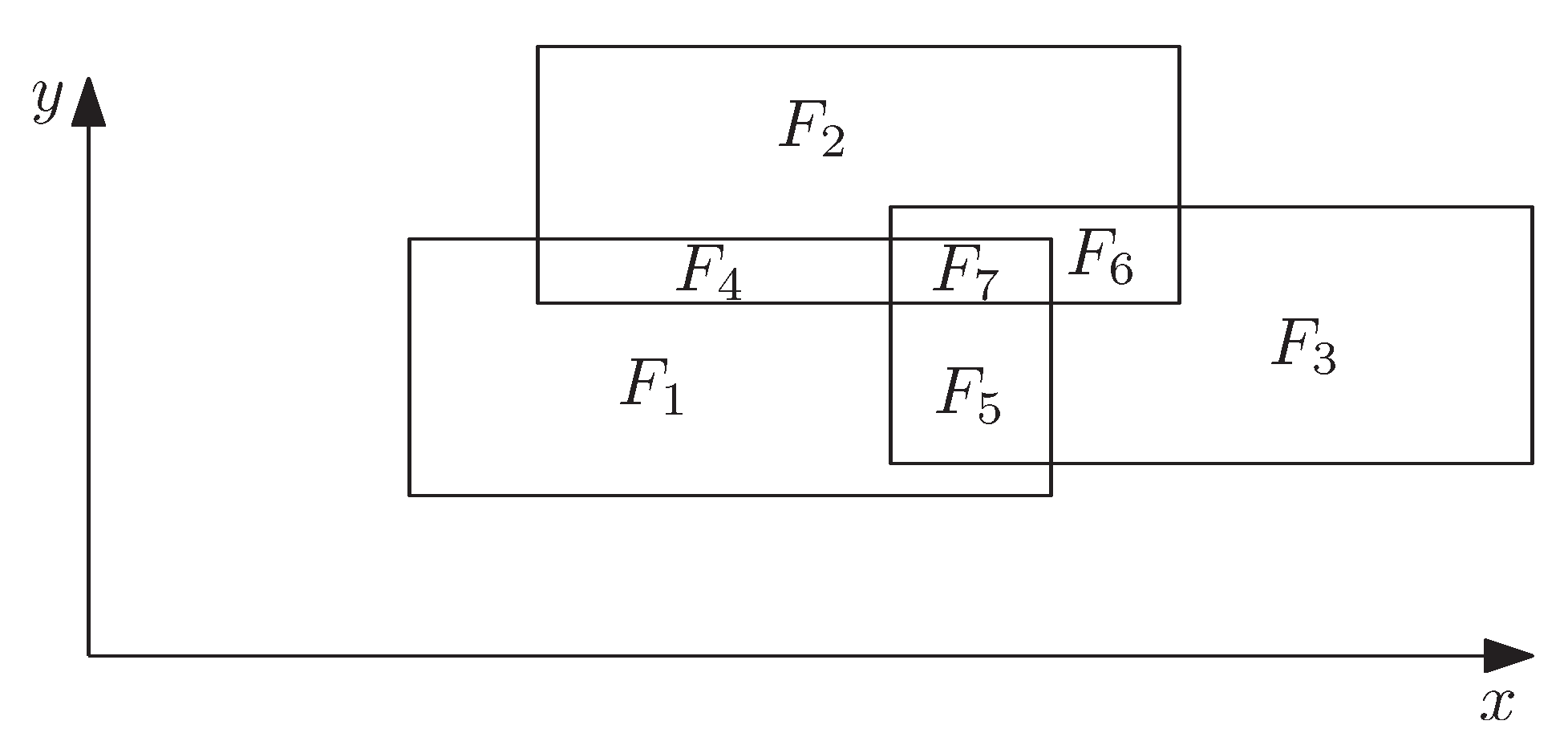
First, to see that the ILP formulation with Constraint (3) is rather weak, suppose that we need to solve the instance in Figure 5 with the three rectangular labels , , and , each of which belongs to a different feature. To rule out intersections between the labels, we need to instantiate Constraint (3) three times: , , and . Assuming unit weights (that is, for each ), an optimal integer solution is obtained by setting an arbitrary x-variable to 1. Such a solution has objective value 1. In the LP-relaxation, however, we can satisfy Constraint (3) by setting each of the three x-variables to . This solution has objective value , which is a rather poor estimate for the objective value of .
To strengthen our ILP formulation, we avoid label–label conflicts by setting up Constraint (8) with a particular choice of and . More precisely, we restrict to the origin of the coordinate system. This yields for every label , and the arrangement simply results from an overlay of all labels. By setting , we achieve that every face of is covered by at most one label. Hence, no two labels intersect. Using the same example as before, we obtain an arrangement of faces (not counting the unbounded exterior face); see Figure 6. This results in the following seven instantiations of Constraint (8): ; ; ; ; ; ; . Note that the inequality for implies all other inequalities, thus we can avoid intersections between labels with a single constraint. We say that the constraint for is a non-dominated constraint, whereas each other constraint is by the constraint for . In the LP-relaxation, this constraint clearly forbids setting all variables to . It turns out that, in this example, an optimal solution of the LP-relaxation (for example, the solution ) has the same value (that is, 1) as an optimal solution of the ILP.
Generally, the LP-relaxation of the ILP with this constraint yields an upper bound that is at least as tight as the upper bound yielded by the LP-relaxation of the ILP with Constraint (3). Therefore, it is a promising variant. To summarize, we define the following two ILP formulations, ILP 1 and ILP 2, which both encode the labeling problem with our model extensions.
- ILP 1 consists of
- ILP 2 differs from ILP 1 only as follows:
3.6. An LP-Based Rounding Heuristic
The existing ILP solvers allow us to compute optimal solutions to our model, yet the running time may be high. Additionally, to achieve a polynomial running time, we have developed an LP-rounding heuristic. This is based on the general assumption that a variable has similar values in an optimal solution of an ILP and in an optimal solution of the corresponding LP. Algorithm 1 summarizes our approach. We first solve the LP-relaxation of an ILP for our problem, that is, ILP 1 or ILP 2. This can be done with the same software (for example, CPLEX or Gurobi) that is used for solving ILPs. For example, the LP-relaxation can be solved with the simplex algorithm, which is an important subroutine in almost every ILP solver. Once we have obtained an optimal solution of the LP-relaxation, we sort the x-variables in decreasing order of their values. Then, we iterate through the resulting sequence of variables. In each iteration, we select the label corresponding to the current variable if this does not introduce a violation of a constraint. To identify a constraint violation when selecting a label ℓ, we check all constraints in which the variable occurs. Note that the number of such constraints can be quadratic in the number of labels. Since the for-loop in Algorithm 1 has iterations and each iteration may take time for checking the constraints, the algorithm needs time in the worst case (not including the time for solving the LP). In practice, however, we expect a better running time since each variable occurs only in a linear number of constraints if the given set of labels is not too dense.
| Algorithm 1: LP-based rounding heuristic |
 |
4. Experimental Results
We implemented our algorithms in Java and tested them with respect to their running times in practice and the quality of their results. Our code is provided online as supplementary material to our article. We used the solver Gurobi (www.gurobi.com, version 6.0) to solve our ILPs and LPs. All tests were performed on a Windows PC with an Intel Core i7-3770 CPU and 16 GB of RAM.
For setting up Constraint (8), which we defined based on the arrangement , we tested two different methods. Our first method computes a geometric representation of in terms of polygons with Cartesian coordinates. This is accomplished with the Java library JTS topology suite. However, this method turned out to be rather inefficient—in fact, for our densest problem instances, the time for computing was the dominating part of the total running time. Therefore, we implemented a second method for the special case that the region is an axis-aligned rectangle. For this, we used our own implementation of a plane-sweep algorithm that returns a list of all the faces of that correspond to non-dominated instances of Constraint (8). The algorithm does so without computing the polygonal boundaries of the faces. For each face f that it returns, it yields the list of labels for it. This method turned out to be much more efficient since it gets along with a minimum of geometric computations. The results that we present in this section were computed with this second method.
The instances for our tests were constructed based on point sets of different sizes, which were either randomly generated or retrieved from the Internet.
We conducted two test series with randomly generated instances, in which we defined four label candidates for each point according to the four-position model. In the first test series, we gradually increased the number of labels without changing their spatial density, which means that we increased the available area linearly with ; see Section 4.1. In the second test series, we gradually increased the number of labels without changing the available area; see Section 4.2. Finally, we present our experiments with real-world data, in which we tested both the four-position model and the eight-position model; see Section 4.3.
4.1. Randomly Generated Instances of Constant Density
In the first test series, we tested our methods for randomly generated instances with point features and rectangular labels. More precisely, for each instance, we sampled the points uniformly at random in the square , which implies on average one point per unit area, and we generated four rectangular labels of width 1 and height for each point, using the four-position model. Afterwards, we slightly enlarged the rectangles, by offsetting their sides units outwards. Due to this enlargement, any two labels for the same point intersect. As a consequence, Constraint (4) is automatically satisfied in every solution without intersecting labels. Therefore, we did not instantiate that constraint in our tests.
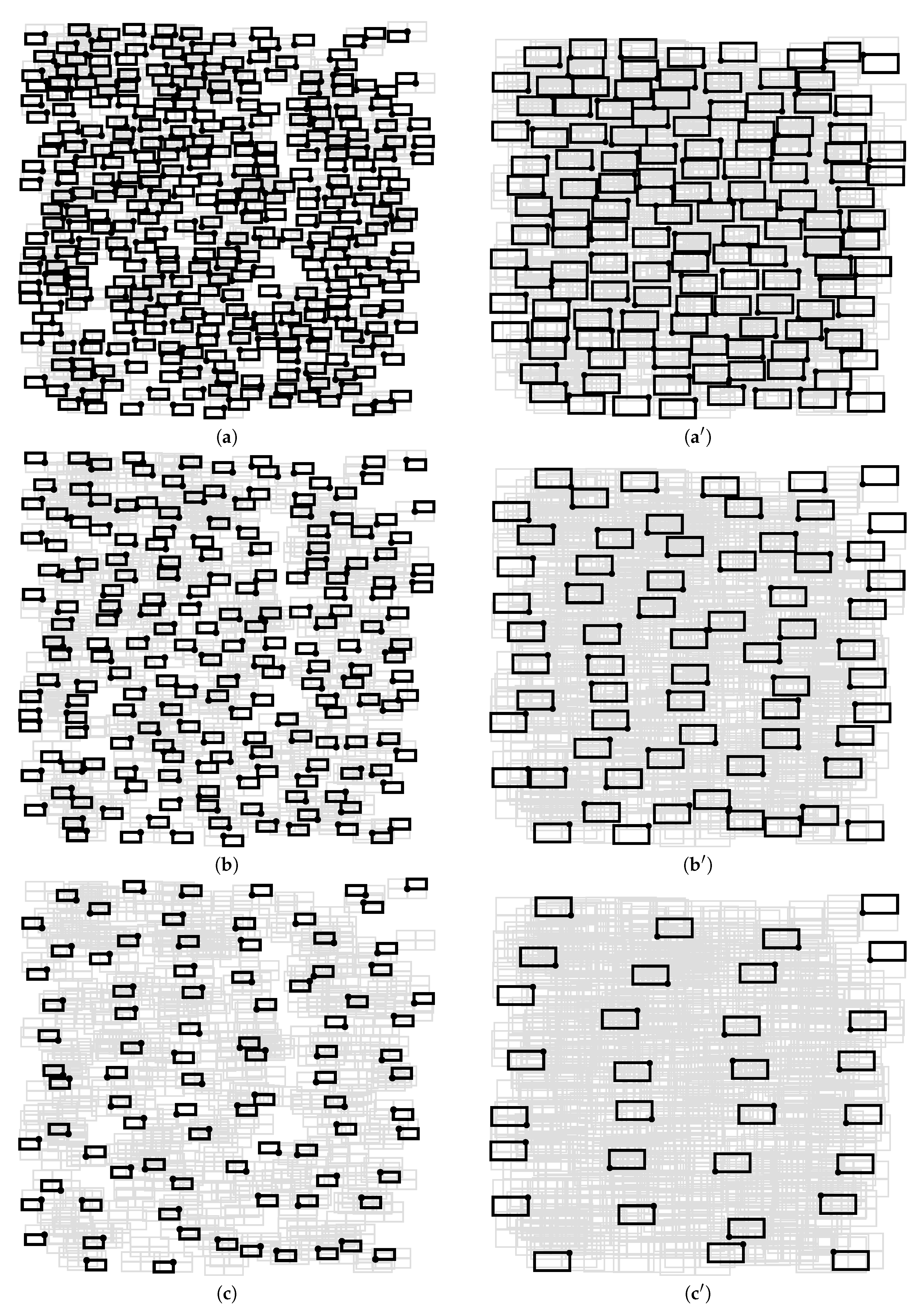
To define the quality of a solution, we sampled the weight for each label uniformly at random from the interval . Furthermore, we defined and , which influences the cost that we charge if a labeled point is within distance from a label of a different point. We tested Constraint (8) with different settings. In these tests, we observed that the desired effect is achieved already when defining as a relatively small region and assigning small values to . That is, while we obtained very densely packed solutions without our model extensions (see Figure 7a), we were able to loosen up the masonry-like layout of the labels by using Constraint (8) with a square of size for and with (see Figure 7b). By defining as a square of size , we were able to further decrease the label density (see Figure 7c).
We computed optimal solutions for all our instances using both ILP formulations of our extended model, that is, ILP 1 and ILP 2. Furthermore, we solved each of our problem instances without our model extensions.
Table 1 and Table 2 summarize the running times of our experiments and the performance of our rounding heuristic in comparison to the exact method. While, for the results in Table 1, we let be a square of size , we used a square of size for the results in Table 2. In both tables, the running times with ILP 1 and ILP 2 (which includes the time for setting up the objective and the constraints and solving the ILP) are summarized in the third and fourth column, respectively. These results do not reveal a clear advantage of one ILP formulation over the other. The longest running times were observed when solving the instances with 1600 labels and a square of size for with ILP 1; see the last row and third column of Table 4. With slightly more than 3 min, however, this running time was still moderate. When we tested our heuristic with the two ILP formulations, however, we observed a clear advantage of ILP 2 (that is, the alternative (strong) constraint formulation from Section 3.5) with respect to the objective value that we achieved. We refer to the ratio between the objective value of a solution and the optimal objective value as the quality of that solution. When combining the heuristic with ILP 2, we obtained solutions of very high quality, that is, they were merely 5% worse than the optimal solutions obtained with the exact solver; see the last columns of Table 1 and Table 2. For each of our instances, the heuristic needed only few seconds.
To summarize, our tests for instances of a rather moderate point density show that the methods with ILP 1 and ILP 2 allow us to solve instances of 1600 labels with proof of optimality and in reasonable time. Our LP-based rounding heuristic needs only few seconds for the same instances and, when used in conjunction with ILP 2, yields solutions with high objective values.
4.2. Randomly Generated Instances of a Constant Spatial Extent
In the second test series, we repeated our experiments from the first test series, except that this time we did not increase the size of the square containing all points. We sampled all points uniformly at random into the square and thus gradually increased the spatial density of the labels. Table 3 and Table 4 summarize these tests. Figure 7 (right) shows three solutions for one of our densest instances.
By sampling more points into the same area, both the size of the arrangement and the number of y-variables grow quadratically with . Therefore, in almost all cases, the running times were higher than in the first test series, which we documented in Section 4.1 (compare Table 1 with Table 3 and Table 2 with Table 4). Nevertheless, we were still able to solve all instances with proof of optimality. When letting be a square of size and solving the largest instances with ILP 2, the method needed on average 792.4 s, that is, slightly more than 13 min. This turned out to be the setting with which our method performed worst. When using the heuristic with ILP 2, we obtained solutions with objective values above 90% of the optimal objective value. When letting be a square of size , however, we obtained relatively low values compared to the other settings; see the last column of Table 3 with the lowest value of 90.4% in the last row.
To summarize, for very dense instances, our exact and heuristic methods are slower than for less dense instances. The running times of our exact methods may still be tolerable for the production of static maps, but, for time-critical applications, a processing time of 10 min for an instance of 400 point features can be unacceptable. Our experiments confirm the finding from Section 4.1 that the heuristic should be used in conjunction with the stronger ILP formulation, that is, ILP 2.
4.3. Instances with Existing Point Data
We tested our method for a global data set of populated places, which we took from the website Natural Earth (www.naturalearthdata.com/downloads/10m-cultural-vectors/10m-populated-places). This data set (version 3.3.1) contains 7322 points with attributes such as city names and a lower and an upper estimate (“pop_min” and “pop_max”, resp.) of each place’s population. Based on these estimates, ranks (“rank_min” and “rank_max”, resp.) have been assigned to the points, where each rank is an integer number in the range from 0 to 14. To ensure strictly positive weights and to give a high preference to labeling large cities, we define the weight of each label ℓ as
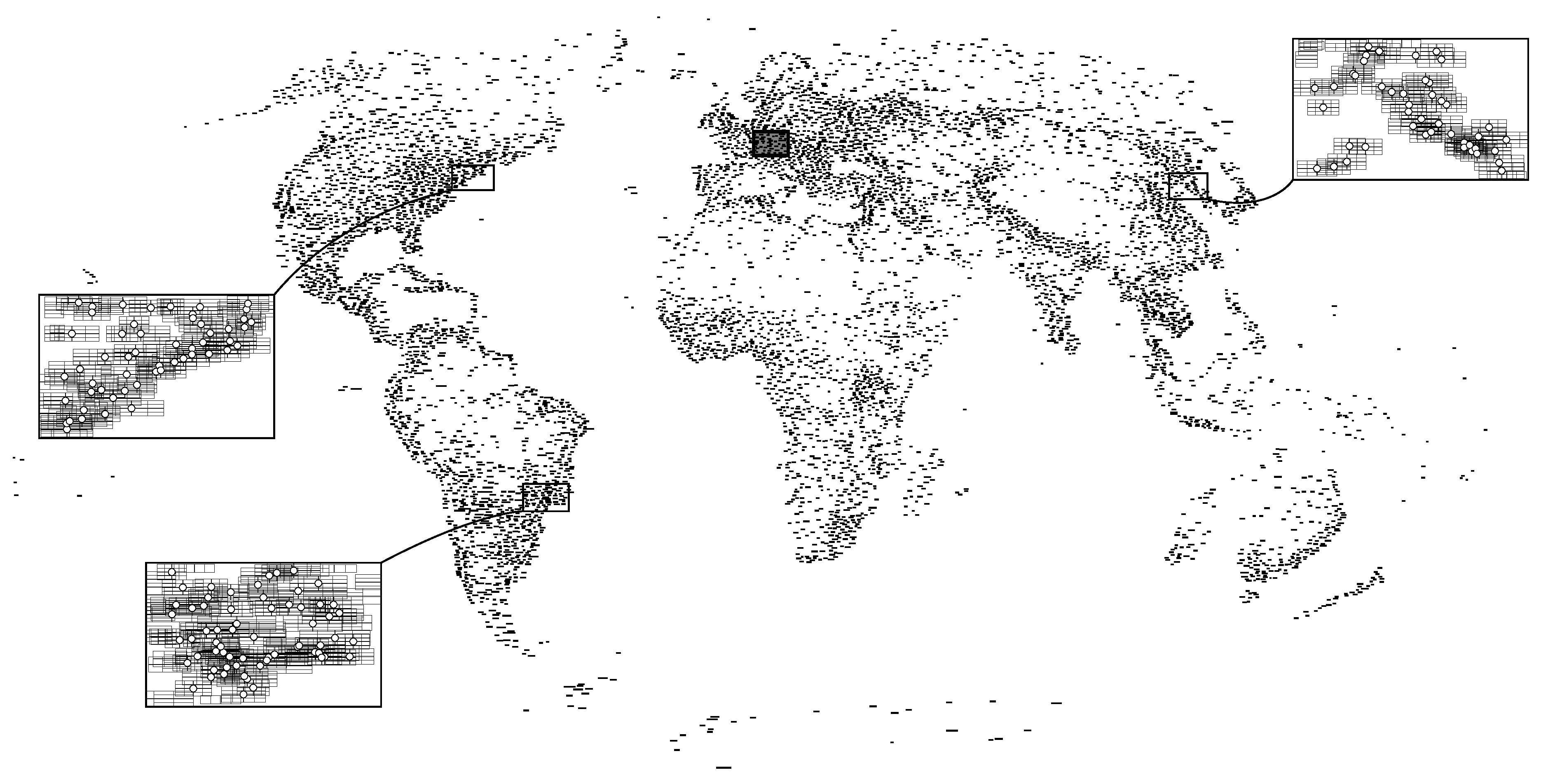
We projected the data set with a Mollweide projection and scaled it such that one unit of a screen coordinate system (that is, one pixel) corresponds to 2000 m in reality. For the label text, we rendered each place’s name using the font Times New Roman with font size 12. The bounding box of the rendered text was placed at different positions relative to the corresponding point, using the four-position model in a first test and the eight-position model in a second test. Each of the resulting rectangles was offset 0.5 units outwards to define the labels. This yielded rectangular labels with a height of approximately 32.4 km in world coordinates. Figure 8 shows a labeling for this instance.
To penalize ambiguous label–point associations, we set units (that is, 8 km) and . With this setting, our algorithm identified 8355 potential interferences between the labels with the four-position model and 25,755 with the eight-position model (which corresponds to the number of y-variables in our model). To avoid densely packed solutions in which the labels form a pattern that looks like a wall of densely packed bricks (see Figure 3), we required that every axis-aligned square of units must not intersect more than labels.
With the defined setting and ILP 1, we were able to compute a solution that is optimal according to our extended model in 229.4 s when using the four-position model and in 2092.8 s (that is, in slightly more than half an hour) with the eight-position model. The tests with ILP 2 and our heuristic confirmed our results from the previous section. That is, the exact method is slower with ILP 2, but combining the heuristic with ILP 2 instead of with ILP 1 offers a clear advantage in terms of quality; see Table 5.
To assess the optimal solutions of our model with respect to cartographic quality, we also solved the basic ILP for both the four-position model and the eight-position model. That is, we did not consider the y-variables in the objective function and we did not explicitly restrict the number of labels that intersect an axis-aligned square of units. Because of the height of our labels (which is approximately 16 units) and assuming that every label is wider than high, however, such a square can intersect with at most nine mutually non-intersecting labels.
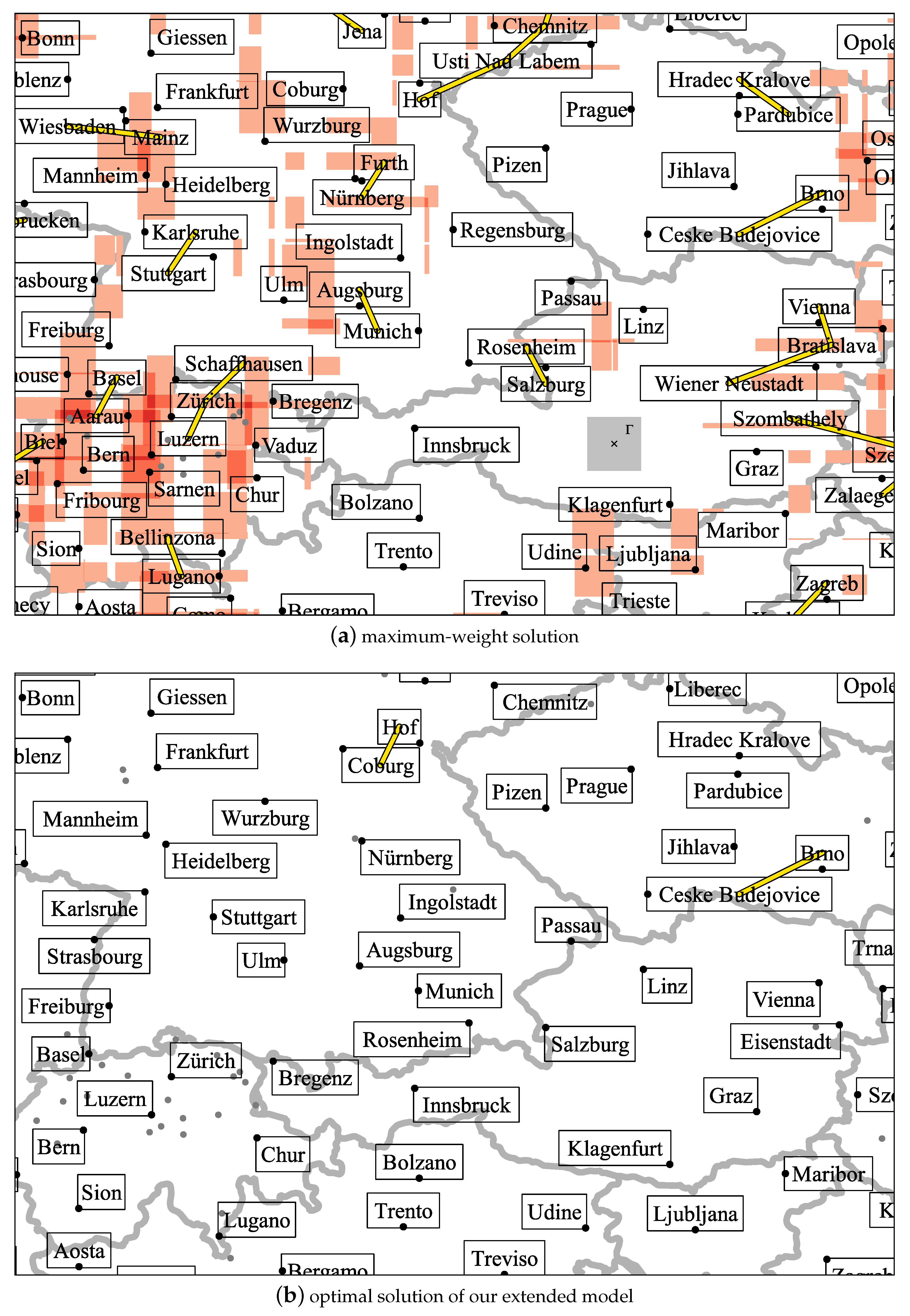
A solution of maximum weight, which we computed with the basic ILP, is shown in Figure 9a, and a solution that is optimal with respect to our extended model in Figure 9b.
We clearly observe that, in the maximum-weight solution, more places are labeled. Especially the north of Switzerland is almost completely covered with labels in Figure 9a, which can be undesirable. Placing the center of to the left of the Swiss town Zürich would cause intersections with the five labels for Aarau, Basel, Schaffhausen, Zug, and Zürich (which is indicated with dark red color in Figure 9a). Moreover, Figure 9a contains many interferences in the sense that a label could be associated with a wrong point. The label for Bratislava, for example, could be associated with the point representing Vienna. While in Figure 9b, more places are unlabeled (for example, Bellinzona and Fribourg), there is no point where centering a square of units would intersect more than two labels. Consequently, the labels appear to be much less densely packed. There are also two interferences in Figure 9b, for example, the label for Coburg could be associated with the point representing Hof. Overall, however, the number of interferences because of ambiguous label–point associations was greatly reduced.
We also assessed the quality of each solution in terms of the total weight of the labeling (that is, the objective function of the basic ILP) and the cost for interferences between labels. With the four-position model, our extended model resulted in a labeling of 0.7% less total weight compared to the solution of the basic ILP. The cost for interferences, however, was reduced by 82.1% with the extended model. Similarly, with the eight-position model, the weight of the labeling decreased by 0.5% and the cost for interferences by 85.0% when using the extended model instead of the basic model. This means that a relatively small weight reduction can lead to very large improvements in terms of interferences.
5. Conclusions
We have presented a new exact method for point-feature labeling that allows for the consideration and avoidance of ambiguous label–point associations and labels that are packed too densely. We are far from claiming that we have applied our model with a perfect choice of its parameters. A perfect setting of the parameters does not exist since different maps serve different purposes that require different densities of labels with place names—a weather map, for example, needs only few labels to provide sufficient geographical context, whereas a topographic map should display detailed information on places. By choosing the parameters of our model, however, we can effectively control the graphic density, thus our model extensions offer the possibility of producing maps for different applications.
If the input point set is not too dense, our ILP-based approach yields optimal solutions in reasonable time. For a world map with 7322 places and four label candidates for each point, we were able to compute an optimal labeling in less than 11 min, and in slightly more than half an hour when defining eight label candidates per point. We have also presented an LP-based rounding heuristic, which yields near-optimal solutions for our instances.
With respect to cartographic quality, it would be interesting to see how our model extension performs with a more sophisticated weight function such as the one by Rylov and Reimer [9]. For example, it would be reasonable to reduce the weight of a label candidate if it occludes much information of the map background. We also think that our model of graphic density could be extended. The current model allows us to bound the graphic density from above such that it does not exceed a given threshold. However, it may be reasonable to allow for a higher graphic density, for example, in highly populated areas. A reasonable approach to this problem would be to define an ideal graphic density for each point in the plane and to penalize deviations from this ideal graphic density in the objective function.
Supplementary Materials
The benchmark sets and the code used for the experiments in this paper are available at www.mdpi.com/2220-9964/6/11/342/s1.
Acknowledgments
This publication was funded by the German Research Foundation (DFG) and the University of Würzburg in the funding programme Open Access Publishing.
Author Contributions
J.H. initiated this research project, implemented the algorithms, did the experiments, and wrote most of the paper. A.W. contributed to the development of the mathematical model, gave feedback on the write-up, and helped polishing it.
Conflicts of Interest
The authors declare no conflicts of interest.
References
- Wolff, A.; Knipping, L.; van Kreveld, M.; Strijk, T.; Agarwal, P.K. A Simple and Efficient Algorithm for High-Quality Line Labeling. In Innovations in GIS VII: GeoComputation; Atkinson, P.M., Martin, D.J., Eds.; Taylor & Francis: London, UK, 2000; Chapter 11; pp. 147–159. [Google Scholar]
- Rylov, M.; Reimer, A. A Practical Algorithm for the External Annotation of Area Features. Cartogr. J. 2017, 54, 61–76. [Google Scholar] [CrossRef]
- Haunert, J.H.; Wolff, A. Beyond Maximum Independent Set: An Extended Model for Point-Feature Label Placement. In Proceedings of the International Archives of the Photogrammetry, Remote Sensing and Spatial Information Sciences, XXIII ISPRS Congress, Prague, Czech Republic, 12–19 July 2016; Volume XLI-B2, pp. 109–114. [Google Scholar]
- Zoraster, S. Integer Programming Applied to the Map Label Placement Problem. Cartographica 1986, 23, 16–27. [Google Scholar] [CrossRef]
- Agarwal, P.K.; van Kreveld, M.; Suri, S. Label Placement by Maximum Independent Set in Rectangles. Comput. Geom. Theory Appl. 1998, 11, 209–218. [Google Scholar] [CrossRef]
- Ribeiro, G.M.; Mauri, G.R.; Lorena, L.A.N. A Lagrangean Decomposition for the Maximum Independent Set Problem Applied to Map Labeling. Oper. Res. 2011, 11, 229–243. [Google Scholar] [CrossRef]
- Bertin, J. Semiology of Graphics: Diagrams, Networks, Maps, 1st ed.; The University of Wisconsin Press: Madison, WI, USA, 1983. [Google Scholar]
- Kern, J.P.; Brewer, C.A. Automation and the Map Label Placement Problem: A Comparison of Two GIS Implementations of Label Placement. Cartogr. Perspect. 2008, 60, 22–45. [Google Scholar] [CrossRef]
- Rylov, M.; Reimer, A. A Comprehensive Multi-criteria Model for High Cartographic Quality Point-Feature Label Placement. Cartographica 2014, 49, 52–68. [Google Scholar] [CrossRef]
- Formann, M.; Wagner, F. A Packing Problem with Applications to Lettering of Maps. In Proceedings of the 7th Annual ACM Symposium on Computation Geometry (SoCG’91), North Conway, NH, USA, 10–12 June 1991; pp. 281–288. [Google Scholar]
- Achterberg, T.; Wunderling, R. Mixed Integer Programming: Analyzing 12 Years of Progress. In Facets of Combinatorial Optimization: Festschrift for Martin Grötschel; Jünger, M., Reinelt, G., Eds.; Springer: Berlin, Germany, 2013; pp. 449–481. [Google Scholar]
- Nemhauser, G.L.; Wolsey, L. Integer and Combinatorial Optimization; John Wiley & Sons: Hoboken, NJ, USA, 1988. [Google Scholar]
- Yoeli, P. The Logic of Automated Map Lettering. Cartogr. J. 1972, 9, 99–108. [Google Scholar] [CrossRef]
- Imhof, E. Positioning Names on Maps. Am. Cartogr. 1975, 2, 128–144. [Google Scholar] [CrossRef]
- Alinhac, G. Cartographie Théorique et Technique; Institut Géographique National: Paris, France, 1962; Chapter IV. [Google Scholar]
- Doerschler, J.S.; Freeman, H. An Expert System for Dense-Map Name Placement. In Proceedings of the 9th International Symposium on Computer-Assisted Cartography (Auto-Carto 9), Baltimore, MD, USA, 2–7 April 1989; pp. 215–224. [Google Scholar]
- Zoraster, S. The Solution of Large 0–1 Integer Programming Problems Encountered in Automated Cartography. Oper. Res. 1990, 38, 752–759. [Google Scholar] [CrossRef]
- Verweij, B.; Aardal, K. An Optimisation Algorithm for Maximum Independent Set with Applications in Map Labelling. In Proceedings of the 7th Annual European Symposium on Algorithms (ESA’99), Prague, Czech Republic, 16–18 July 1999; Springer: Berlin, Germany, 1999; pp. 426–437. [Google Scholar]
- Christensen, J.; Marks, J.; Shieber, S. An Empirical Study of Algorithms for Point-Feature Label Placement. ACM Trans. Graph. 1995, 14, 203–232. [Google Scholar] [CrossRef] [Green Version]
- Wagner, F.; Wolff, A.; Kapoor, V.; Strijk, T. Three Rules Suffice for Good Label Placement. Algorithmica 2001, 30, 334–349. [Google Scholar] [CrossRef]
- Van Kreveld, M.; Strijk, T.; Wolff, A. Point Labeling with Sliding Labels. Comput. Geom. Theory Appl. 1999, 13, 21–47. [Google Scholar] [CrossRef]
- Strijk, T.; van Kreveld, M. Practical Extensions of Point Labeling in the Slider Model. GeoInformatica 2002, 6, 181–197. [Google Scholar] [CrossRef]
- Meng, Y.; Zhang, H.; Liu, M.; Liu, S. Clutter-aware label layout. In Proceedings of the IEEE Pacific Visualization Symposium (PacificVis 2015), Hangzhou, China, 14–17 April 2015; pp. 207–214. [Google Scholar]
- Wu, H.Y.; Takahashi, S.; Poon, S.H.; Arikawa, M. Introducing Leader Lines into Scale-Aware Consistent Labeling. In Advances in Cartography and GIScience: Selections from the International Cartographic Conference 2017; Peterson, M.P., Ed.; Springer International Publishing: Basel, Switzerland, 2017; pp. 117–130. [Google Scholar]
- Been, K.; Nöllenburg, M.; Poon, S.H.; Wolff, A. Optimizing Active Ranges for Consistent Dynamic Map Labeling. Comput. Geom. Theory Appl. 2010, 43, 312–328. [Google Scholar] [CrossRef]
- Raidl, G.R. A Genetic Algorithm for Labeling Point Features. In Proceedings of the International Conference on Imaging Science, Systems, and Technology (CISST’98), Las Vegas, NV, USA, 6–9 July 1998; pp. 189–196. [Google Scholar]
- Ribeiro, G.M.; Lorena, L.A.N. Lagrangean relaxation with clusters for point-feature cartographic label placement problems. Comput. Oper. Res. 2008, 35, 2129–2140. [Google Scholar] [CrossRef]
- Yamamoto, M.; Camara, G.; Lorena, L.A.N. Tabu Search Heuristic for Point-Feature Cartographic Label Placement. GeoInformatica 2002, 6, 77–90. [Google Scholar] [CrossRef]
- Alvim, A.C.F.; Taillard, É.D. POPMUSIC for the Point Feature Label Placement Problem. Eur. J. Oper. Res. 2009, 192, 396–413. [Google Scholar] [CrossRef]
- Bae, W.D.; Alkobaisi, S.; Narayanappa, S.; Vojtechovský, P.; Bae, K.Y. Optimizing Map Labeling of Point Features Based on an Onion Peeling Approach. J. Spat. Inf. Sci. 2011, 2, 3–28. [Google Scholar] [CrossRef]
- Gomes, S.P.; Ribeiro, G.M.; Lorena, L.A.N. Dispersion for the Point-Feature Cartographic Label Placement Problem. Expert Syst. Appl. 2013, 40, 5878–5883. [Google Scholar] [CrossRef]
- Gomes, S.P.; Lorena, L.A.N.; Ribeiro, G.M. A Constructive Genetic Algorithm for Discrete Dispersion on Point Feature Cartographic Label Placement Problems. Geogr. Anal. 2016, 48, 43–58. [Google Scholar] [CrossRef]
- Mauri, G.R.; Ribeiro, G.M.; Lorena, L.A.N. A New Mathematical Model and a Lagrangean Decomposition for the Point-Feature Cartographic Label Placement Problem. Comput. Oper. Res. 2010, 37, 2164–2172. [Google Scholar] [CrossRef]
- Rabello, R.L.; Mauri, G.R.; Ribeiro, G.M.; Lorena, L.A.N. A Clustering Search Metaheuristic for the Point-Feature Cartographic Label Placement Problem. Eur. J. Oper. Res. 2014, 234, 802–808. [Google Scholar] [CrossRef]
- Haunert, J.; Wolff, A. Area aggregation in map generalisation by mixed-integer programming. Int. J. Geogr. Inf. Sci. 2010, 24, 1871–1897. [Google Scholar] [CrossRef]
- Been, K.; Daiches, E.; Yap, C. Dynamic Map Labeling. IEEE Trans. Vis. Comput. Graph. 2006, 12, 773–780. [Google Scholar] [CrossRef] [PubMed]
- De Berg, M.; Cheong, O.; van Kreveld, M.; Overmars, M. Computational Geometry: Algorithms and Applications, 3rd ed.; Springer TELOS: Santa Clara, CA, USA, 2008. [Google Scholar]
Figure 1.
The four label candidates for a point in the four-position model (left) and the additional four label candidates in the eight-position model (right).
Figure 1.
The four label candidates for a point in the four-position model (left) and the additional four label candidates in the eight-position model (right).

Figure 2.
A point p with a label ℓ, which can be misinterpreted as the label for q, since q is within distance from ℓ. When labeling p with ℓ, the label for q can be r, s, or t.
Figure 2.
A point p with a label ℓ, which can be misinterpreted as the label for q, since q is within distance from ℓ. When labeling p with ℓ, the label for q can be r, s, or t.

Figure 3.
(left): a labeling of four labels that intersect a disk of radius ; such a solution can be avoided with our model by defining as a disk of radius centered in and ; (middle): the same situation with a square-shaped region , which is the setting that we used in our experiments; (right): the same situation with a triangular region —we use this setting in the following discussion to show that is not required to be symmetric.

Figure 4.
A label ℓ, a region , and the region . The definition of implies that translating with a vector yields a region intersecting ℓ.
Figure 4.
A label ℓ, a region , and the region . The definition of implies that translating with a vector yields a region intersecting ℓ.

Figure 5.
Three labels , , and with the regions , , and (top) as well as the faces of the arrangement resulting from the overlay of , , and (bottom).
Figure 5.
Three labels , , and with the regions , , and (top) as well as the faces of the arrangement resulting from the overlay of , , and (bottom).
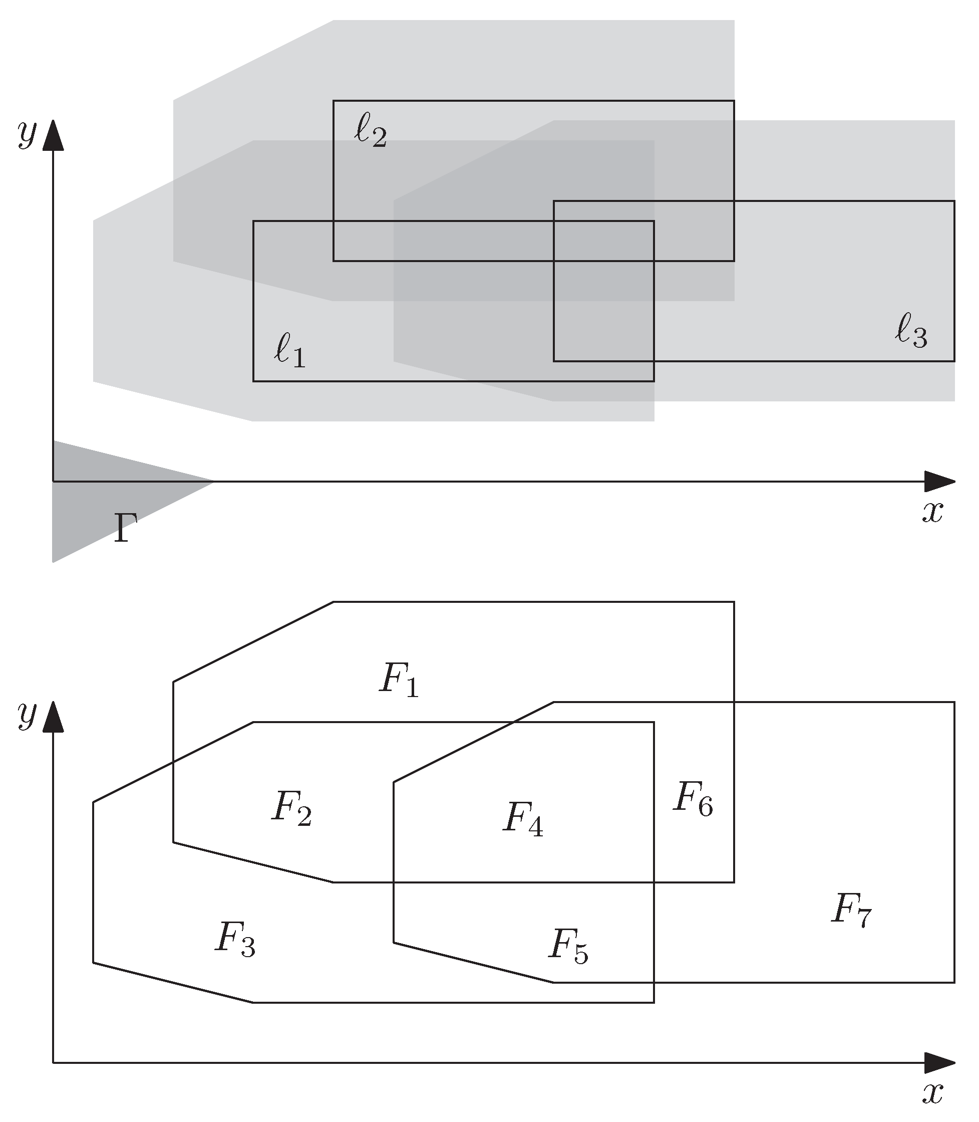
Figure 6.
The seven faces of the arrangement formed by the three labels in Figure 5.
Figure 6.
The seven faces of the arrangement formed by the three labels in Figure 5.

Figure 7.
Different labelings for an instance with 400 points in a square of size (left side) and in a square of size (right side). Selected labels are displayed with black boundaries, unselected labels with gray boundaries. (a, a) maximum-weight solution; (b, b) solution of the extended model; is a square of size and ; (c, c) solution of the extended model; is a square of size and .

Figure 8.
The labels of a solution for the instance that we generated from an existing data set, using the eight-position model. In the three magnified rectangles all point features and label candidates in the corresponding region of the map are displayed. The gray shaded rectangle is magnified in Figure 9.

Figure 9.
The two maps show the same section of two labelings for the instance in Figure 8. Yellow lines represent pairs of labels whose corresponding y-variables have been constrained to 1; only in the second labeling, costs for those variables have been charged to avoid ambiguous label–point associations. Red areas represent points where centering would cause intersections with more than two labels (from light red to dark red: three, four, five intersections). Because of Constraint (8), there are no such areas in the second solution. Unlabeled points are displayed gray and will not be visible in the final map. Country borders were not considered for labeling but are displayed to provide context.

Table 1.
Experimental results for instances with different numbers of points but a constant spatial density of one point per area unit. Four rectangles of size were generated for each point. Every square of size was required to intersect at most two labels. Running times are in seconds CPU time. Every value is the average over ten instances.
| ILP 1 | ILP 2 | ILP 1 & 2 | Heuristic with ILP 1 | Heuristic with ILP 2 | ||||
|---|---|---|---|---|---|---|---|---|
| Time (s) | Time (s) | Quality | Time (s) | Quality | Time (s) | Quality | ||
| 100 | 400 | 0.9 | 1.0 | 100% | 0.4 | 86.7% | 0.5 | 95.9% |
| 200 | 800 | 3.7 | 3.8 | 100% | 0.7 | 87.3% | 0.7 | 95.7% |
| 300 | 1200 | 26.9 | 30.1 | 100% | 1.2 | 86.7% | 1.1 | 95.9% |
| 400 | 1600 | 96.6 | 102.4 | 100% | 1.7 | 86.7% | 1.6 | 94.7% |
Table 2.
Experimental results with the same setting as in Table 1, except that this time every square of size was required to intersect at most two labels.
Table 2.
Experimental results with the same setting as in Table 1, except that this time every square of size was required to intersect at most two labels.
| ILP 1 | ILP 2 | ILP 1 & 2 | Heuristic with ILP 1 | Heuristic with ILP 2 | ||||
|---|---|---|---|---|---|---|---|---|
| Time (s) | Time (s) | Quality | Time (s) | Quality | Time (s) | Quality | ||
| 100 | 400 | 2.4 | 2.2 | 100% | 1.3 | 90.5% | 1.3 | 97.6% |
| 200 | 800 | 7.4 | 7.1 | 100% | 2.7 | 90.0% | 2.6 | 97.6% |
| 300 | 1200 | 43.5 | 46.1 | 100% | 4.5 | 89.2% | 4.4 | 95.3% |
| 400 | 1600 | 190.4 | 127.2 | 100% | 6.3 | 89.7% | 6.1 | 95.4% |
Table 3.
Experimental results for instances with different numbers of points in a constant-sized area of size and four labels of size for each point. Every square of size was required to intersect at most two labels. Running times are in seconds CPU time. Every value is an average over ten instances.
| ILP 1 | ILP 2 | ILP 1 & 2 | Heuristic with ILP 1 | Heuristic with ILP 2 | ||||
|---|---|---|---|---|---|---|---|---|
| Time (s) | Time (s) | Quality | Time (s) | Quality | Time (s) | Quality | ||
| 100 | 400 | 0.9 | 0.9 | 100% | 0.4 | 86.7% | 0.4 | 95.6% |
| 200 | 800 | 17.6 | 19.2 | 100% | 2.0 | 88.6% | 2.0 | 93.9% |
| 300 | 1200 | 185.9 | 229.2 | 100% | 6.4 | 88.1% | 6.2 | 93.2% |
| 400 | 1600 | 698.5 | 792.4 | 100% | 14.2 | 87.8% | 14.3 | 90.4% |
Table 4.
Experimental results with the same setting as in Table 3, except that this time every square of size was required to intersect at most two labels.
Table 4.
Experimental results with the same setting as in Table 3, except that this time every square of size was required to intersect at most two labels.
| ILP 1 | ILP 2 | ILP 1 & 2 | Heuristic with ILP 1 | Heuristic with ILP 2 | ||||
|---|---|---|---|---|---|---|---|---|
| Time (s) | Time (s) | Quality | Time (s) | Quality | Time (s) | Quality | ||
| 100 | 400 | 2.4 | 2.2 | 100% | 1.3 | 90.5% | 1.3 | 97.6% |
| 200 | 800 | 18.0 | 16.2 | 100% | 8.6 | 94.2% | 8.4 | 98.3% |
| 300 | 1200 | 72.6 | 59.1 | 100% | 31.3 | 93.6% | 30.7 | 98.1% |
| 400 | 1600 | 189.4 | 153.1 | 100% | 81.3 | 93.9% | 79.2 | 95.7% |
Table 5.
Experimental results for the data set of 7322 places from the Internet. The first row refers to experiments with the four-position model; for the second row, the eight-position model was used.
Table 5.
Experimental results for the data set of 7322 places from the Internet. The first row refers to experiments with the four-position model; for the second row, the eight-position model was used.
| ILP 1 | ILP 2 | ILP 1 & 2 | Heuristic with ILP 1 | Heuristic with ILP 2 | |||||
|---|---|---|---|---|---|---|---|---|---|
| pos. | Time (s) | Time (s) | Quality | Time (s) | Quality | Time (s) | Quality | ||
| 7322 | 4 | 29,288 | 229.4 | 463.0 | 100% | 5.2 | 89.9% | 5.9 | 96.8% |
| 7322 | 8 | 58,576 | 2092.8 | 31,770.0 | 100% | 30.6 | 89.6% | 28.7 | 96.8% |
© 2017 by the authors. Licensee MDPI, Basel, Switzerland. This article is an open access article distributed under the terms and conditions of the Creative Commons Attribution (CC BY) license (http://creativecommons.org/licenses/by/4.0/).
Share and Cite
MDPI and ACS Style
Haunert, J.-H.; Wolff, A. Beyond Maximum Independent Set: An Extended Integer Programming Formulation for Point Labeling. ISPRS Int. J. Geo-Inf. 2017, 6, 342. https://doi.org/10.3390/ijgi6110342
AMA Style
Haunert J-H, Wolff A. Beyond Maximum Independent Set: An Extended Integer Programming Formulation for Point Labeling. ISPRS International Journal of Geo-Information. 2017; 6(11):342. https://doi.org/10.3390/ijgi6110342
Chicago/Turabian StyleHaunert, Jan-Henrik, and Alexander Wolff. 2017. "Beyond Maximum Independent Set: An Extended Integer Programming Formulation for Point Labeling" ISPRS International Journal of Geo-Information 6, no. 11: 342. https://doi.org/10.3390/ijgi6110342
Note that from the first issue of 2016, this journal uses article numbers instead of page numbers. See further details here.