Accuracy Assessment of Landform Classification Approaches on Different Spatial Scales for the Iranian Loess Plateau

Abstract

An accurate geomorphometric description of the Iranian loess plateau landscape will further enhance our understanding of recent and past geomorphological processes in this strongly dissected landscape. Therefore, four different input datasets for four landform classification methods were used in order to derive the most accurate results in comparison to ground-truth data from a geomorphological field survey. The input datasets in 5 m and 10 m pixel resolution were derived from Pléiades stereo satellite imagery and the “Shuttle Radar Topography Mission” (SRTM), and “Advanced Spaceborne Thermal Emission and Reflection Radiometer” (ASTER GDEM) datasets with a spatial resolution of 30 m were additionally applied. The four classification approaches tested with this data include the stepwise approach after Dikau, the geomorphons, the topographical position index (TPI) and the object based approach. The results show that input datasets with higher spatial resolutions produced overall accuracies of greater than 70% for the TPI and geomorphons and greater than 60% for the other approaches. For the lower resolution datasets, only accuracies of about 40% were derived, 20–30% lower than for data derived from higher spatial resolutions. The results of the topographic position index and the geomorphons approach worked best for all selected input datasets.

1. Introduction

The description of the Earth’s surface by automatic classifications is important to derive insight into a landscape. Geomorphometry, as a quantitative analysis of landscape structures, is applied in several fields, such as hydrology, geomorphology, soil science, oceanography or civil engineering [1,2]. In practice, this valuable geomorphometric information can be used for map making, digital soil mapping [3,4,5], hydrologic simulations [6,7] and risk potential analysis [8,9]. Furthermore, this information is useful for the estimation of arable land, as well as areas endangered by soil erosion. Likewise, the achieved information allows estimating past landscape evolution [5].

To derive landform classifications, geomorphometric parameters, e.g., slope and curvature, of digital terrain models are used. These values are utilized for landform classification approaches in different ways and a multitude of different algorithms were developed for a systematic landform classification. Most of them are working with different terrain parameters and combinations of them to derive distinct landform types. For this purpose, most approaches use the assumption of landform types distinguishable by a comparison to the corresponding neighboring elements. The first approaches for a digital landform classification were conducted by Pennock et al. [10], who classified seven landform elements from the morphometric parameters slope, plan curvature and profile curvature. Dikau et al. [11] digitalized the landform classification scheme of Hammond [12,13]. Based on Hammond’s work, he calculated three morphometric values for each cell with a surrounding moving window and grouped them into different categories. Finally, he combined them into five different landform types.

In the following decades, a large number of alternative and modified classification methods were presented. Brabyn et al. [14] modified the classification system of Hammond and Dikau. MacMillan et al. [15] enhanced the classification scheme of Pennock et al. [10] and were able to derive 15 different landform classes instead of seven. In addition, more complex decision tree based approaches were tested to achieve a systematic landform classification [16,17]. Furthermore, besides these numerous landform classification schemes with “crisp, unambiguous boundaries” [18], fuzzy classification methods were introduced [18,19]. To consider the problem that different landform types mostly vary strongly in their sizes, Weiss [20] has developed the topographic position index (TPI). The TPI measures relative height positions of a certain point compared to its surrounding area in two different window sizes, whereas other approaches mostly use only one size for calculation. Thus, this approach is more suitable for heterogeneous landscapes [21]. Another promising approach was conducted by Jasiewicz and Stepinski [22]. Their geomorphons approach creates ternary patterns as a set of possible morphological landscape types from elevation differences in a certain neighborhood.

To take advantage of the segmentation technique over pixel based classification methods, Drǎguţ and Blaschke [23] introduced a new object-based approach. Pixel-based approaches ignore contextual information and only consider values of individual pixels in the classification process. In contrast, object-based approaches use segmentation algorithms prior to the classification to partition the data into sematic objects, which are much more able to divide the landscape in a comprehensible way. Therefore, object based image analysis (OBIA) approaches became very popular in geomorphometry and the number of applied approaches increased in the last decade [24,25,26,27].

Recently, all developed approaches were applied to many different thematic fields and landscapes. They have also become essential for mapping of natural landscapes at different scales. Besides classifications of terrestrial landscape [28] or undersea topography [29] on global scales, also small scale distinct landforms such as gullies [26], drumlins or volcanoes [24,30] were classified. All these approaches show very promising results. However, a thorough evaluation and comparison of the landform classifications schemes is missing. In addition, it is rarely shown how different scales and input datasets overall work with these approaches. The questions of accuracy and scaling arise in particular for areas with stronger relief variation as such landscapes are more sensitive for changes in digital elevation model (DEM) resolutions [31]. Generally, most experiences indicate that DEM pixel resolutions between 5 m and 30 m are most suitable for landform classifications [32,33]. Likewise, input terrain datasets in a higher spatial resolution are available, as satellites nowadays are enabled to record stereo-views of an area. This optical imagery for the derivation of DEMs now achieved a submeter pixel resolution, comparable to already available datasets derived by airborne laser scanning (LiDAR). Furthermore, a global DEM with a 12 m pixel resolution will be available from the TanDEM-X mission, which incorporated two radar satellites and is nearly finished [34].

In this contribution, the comparison of four different landform classification approaches was conducted by three different input datasets for a remote region, which is characterized by a strongly dissected relief, the Iranian loess plateau. The input datasets are the publicly available DEMs of the “Shuttle Radar Topography Mission” (SRTM) and “Advanced Spaceborne Thermal Emission and Reflection Radiometer” (ASTER) (30 m pixel resolution) and two digital elevation models derived from Pléiades stereo imagery aggregated to a 5 m and 10 m pixel resolution. Based on the presented approaches by Dikau et al. [11], Weiss [20], Jasiewicz and Stepinski [22], as well as Drǎguţ and Blaschke [23], landforms were classified in four different ways for each digital elevation model. These methods were applied in two different study areas of the Iranian loess plateau. Both study sites have slightly varying relief characteristics. One is situated in the western part of the loess plateau and has a strongly dissected relief with small valleys and steeply rising hills. The second study area has a flatter relief with some deeply incised valleys and is located in the eastern part of the plateau. To evaluate the results of the conducted landform classifications, geo-located pictures taken on a field campaign in this area were used. The accuracy of the DEMs themselves are compared to measurements of DGPS profiling. However, the precision and accuracy of the DEMs is not considered here, due to the accessibility of the area and only relative heights are used in the selected approaches.

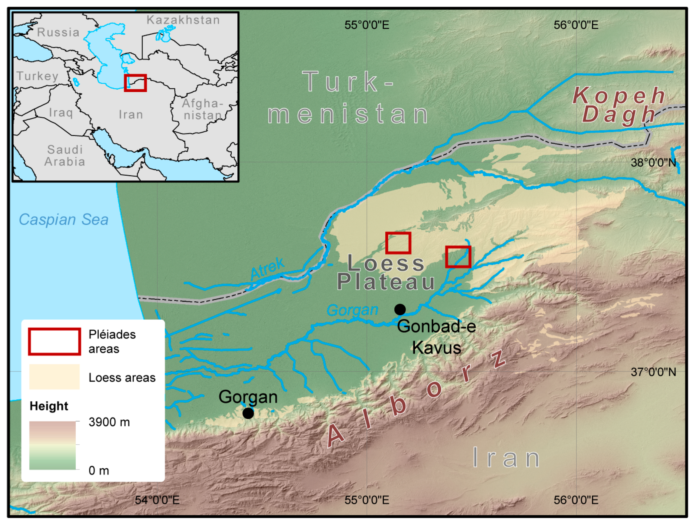
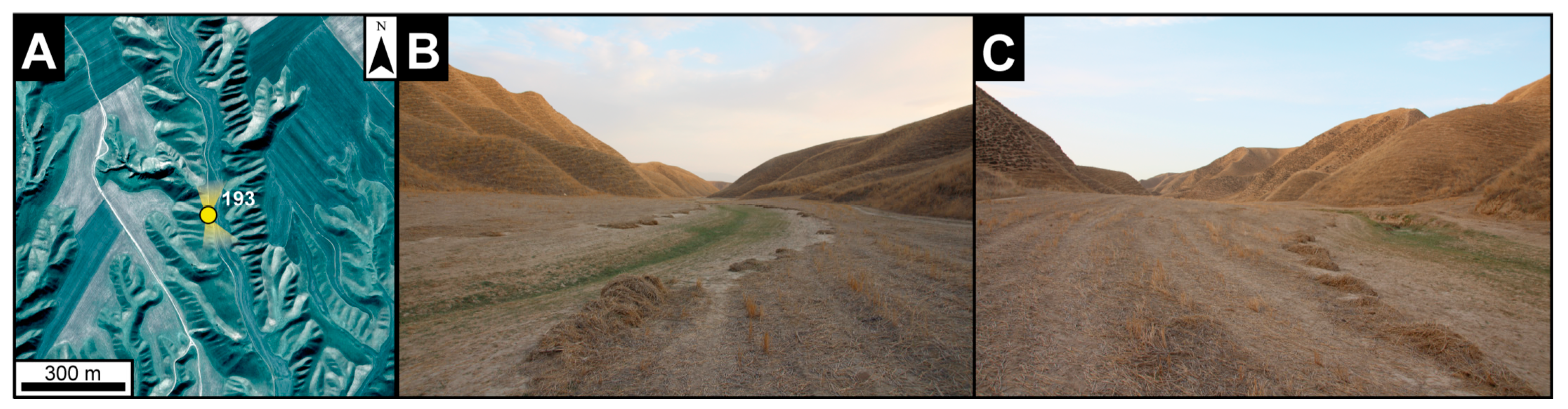
2. Study Area

The Iranian loess plateau is a unique landscape covered by mineral dust, up to at least 70 m thick [35]. Recent sedimentological and geochronological investigations show that these loess deposits have high value as records of Quaternary landscape evolution and climate change. These deposits provide a link between the loess deposits in Southeastern Europe and Central Asia [35,36,37,38]. However, little information is available on its soil, plant cover and the geomorphological evolution of the plateau, as well as on potentials and problems in land use.

The loess plateau covers an area of about 2250 km² in the Turkmen steppe of northern Iran (Figure 1). It is located at altitudes between about 45 m and 300 m above mean sea level. The base of the loess plateau belongs to the western part of the Kopeh Dagh Mountains. It is dissected in several fault blocks [39]. Differential tectonic uplift is expressed in several escarpments and in the sudden altitudinal rise at the boundary of the plateau. Tectonic uplift triggered deep erosion and valley incision into the loess and underlying strata, causing the pronounced relief of the loess plateau. It is characterized by steep slopes frequently dissected by deeply incised v-shaped side-valleys opening to larger valleys with broad floors. Both types are dry valleys with episodic runoff. The ridges in between the valleys rise to about 80 m above the valley floors and mostly consist of loess. Frequent loess wells, sinkholes, pipes and gullies reflect intense erosion processes at the land surface and below. Small scarp faces and hummocky toes indicate local slumping. In addition, the slope surfaces are covered by dense networks of sheep and goat tracks related to severe overgrazing in the area [38].

3. Materials and Methods

3.1. Low Resolution Digital Elevation Models

For the comparison of the different landform classifications the two global digital elevation models (GDEM) in a resolution of 30 m were used. The ASTER sensor is a multispectral imaging system that is on board NASA’s ERA (Earth Observing System) TERRA satellite. The mission was launched in 1999 and was primarily used to collect multispectral data of the Earth [40]. In addition to the multispectral bands, the ASTER sensor has an additional near infrared sensor, which is inclined by 27.6°. These sensors enable a stereoscopic recording according to the “as-track” principle [41]. In 2009, NASA and the Japanese Ministry of International Trade and Industry published a global digital terrain model for the first time. This ASTER global digital elevation model (GDEM) was generated from all stereo images collected. It has a geometric resolution of one arc second, which corresponds to a pixel resolution of about 30 m [42,43]. In 2011, the second version of the ASTER GDEM was released. For the ASTER GDEM 2 used in this contribution, further recordings and enhancements were made available [42]. The accuracy of the ASTER GDEM2 was assessed by the ASTER GDEM Validation Team [42] with an average vertical root mean square error (RMSE) of 8.86 m. Additionally, they reported an RMSE of 6.1 m in flatter areas and of 15.1 m in mountainous regions. The horizontal average error was conducted by a shift of 0.13 arc-seconds to west and 0.19 arc-seconds to north.

In contrast to the previously described passive DEM derivation of the Earth’s surface, it was actively recorded in February 2000 by the SRTM, with the aid of radar systems by the InSAR principle [44]. A DEM from the C-band data was first made available by the USGS in 2003 in a one arc second geometric resolution for the US and a three arc second resolution for the whole Earth. In the course of the year 2015, SRTM data with a geometric resolution of one arc second were made available for the rest of the Earth’s surface. Thus, SRTM data for the region of northern Iran with a geometric resolution of 30 m was also available for the analysis in this contribution. According to Farr et al. [44], the accuracy of the SRTM DEM is determined with an absolute vertical height error of 6.2 m and a relative height error of less than 8.7 m for Eurasia. The horizontal positional accuracy was assessed with a circular absolute geolocation error of 8.8 m.

3.2. High Resolution Digital Elevation Models

In contrast to the previously presented low resolution models, different models in a higher spatial resolution from Pléiades satellite imagery were derived. Pléiades is a satellite system operated by the French Space Center (CNES). The first of the two satellites (Pléiades 1A) was brought into a sun-synchronous orbit on 16 December 2011. One year later, Pléiades 1B followed as the second satellite on 2 December 2012, which completed the system [45]. This system is equipped with optoelectronic CCD scanners, which scan the Earth’s surface transversely to the direction of flight and convert the measured radiation into a measurable electrical signal. It is recorded in a panchromatic channel and four multispectral channels each with five line sensors [46,47]. The line sensors of the panchromatic sensor have a width of more than 6000 pixels and the multispectral sensors have a resolution of 1500 pixels. Thus, the geometric resolution of the satellite is 50 cm in the panchromatic channel and 2 m in the multi-spectral channels [45]. The Pléiades satellites thus belong to the satellite systems with a very high spatial resolution. The panchromatic channel operates in a wavelength range between 480 nm and 830 nm. The positional accuracy is indicated with 8.5 m at nadir and 10.5 m within an angle of 30° [45]. The Pléiades data used in this study are two stereoscopic images, which were recorded over the investigation areas on 28 March 2015, each representing an area of about 10 by 10 km. From these stereo image pairs, the digital terrain models with a pixel resolution of 50 cm were established with the ENVI software. The generation of the Pléiades DEMs was conducted with 25 tie-points for relative orientation. No georeferenced ground control points (GCPs) were used, due to the accessibility. Therefore, only a DEM with relative heights was used in the classification process. From the high-resolution dataset, two datasets with lower pixel resolution (5 m and 10 m) were resampled by the “nearest neighbor” sampling method, which served as the basis for the compilation of the landform classifications.

3.3. Applied Landform Classifications

3.3.1. The Approach of Dikau

Following the approach of Dikau in the 1990s, a stepwise classification was conducted, subdivided in the derivation of slope, local relief and profile type classifications. The whole procedure is computed in ArcMap 10.3 (ESRI) as an automatic tool, implemented with the model builder. Major functions used in ArcMap are slope, focal statistics and map algebra. The first step of this approach is to derive slope classes for each pixel by an adjustable number of neighboring pixels building a rectangle containing a slope of less than 8%. Class breaks are 20%, 50% and 80%, resulting in four classes. The number of neighboring pixels is adjusted to the spatial resolution of the input data, as assigned in

Table 1. Parameters of the moving window sizes in pixels (px) used in this approach for the three different pixel resolutions. Cell size in meters are shown in parentheses.

Moving Window	5 m	10 m	30 m
Slope gradient (rectangle)	3 × 3 (15 m)	3 × 3 (30 m)	3 × 3 (90 m)
Local relief window (circle radius)	15 (75 m)	10 (100 m)	5 (150 m)
Profile type (rectangle)	10 × 10 (50 m)	10 × 10 (100 m)	10 × 10 (300 m)

.

The calculation of the local relief is conducted by building height differences for each pixel and the previously mentioned neighboring pixels (Table 1). In this case, the neighboring pixels are determined by a circle. Classes are built upon the height differences in six classes with class breaks at 30 m, 60 m, 100 m, 150 m and 300 m. Likewise, the profile type is calculated by assigning pixels to upland or lowland and further using classes of flatness, as described before. The assignment to upland or lowland is depending on the position of the pixel in relation to overall height range of the surrounding pixels. A pixel with a height higher than the half of the height range of all pixels is in upland class, a pixel with a height smaller than the half of the height range of all pixels is in the lowland class. Four classes are built by the combination of these calculations, where low- or upland pixels with an amount of slope pixels smaller or higher than 75% are used.

All possible classes of each classification were serially numbered from one to four for the slope and profile type classification and from one to six for the local relief classification. Consequently, each pixel became three numbers depending on their assigned class. A combination of these results in 96 possible combinations for each pixel (

Table 2. Reclassification scheme of the derived landform subclasses to final landform classes.

Landform Sub-Classes Code	Landform Type
111, 112, 121, 122, 131, 132, 141, 142, 151, 152, 161, 162, 211, 212, 221, 222	Plains
113, 114, 123, 124, 133, 134, 143, 144, 153, 154, 163, 164, 213, 214, 223, 224	Plateau
231, 232, 233, 234, 241, 242, 243, 244, 251, 252, 253, 254, 261, 262, 263, 264, 311, 312, 313, 314, 321, 322, 323, 324, 331, 332, 333, 334, 341, 342, 343, 344, 351, 352, 353, 354, 361, 362, 363, 364	Irregular Plains
411, 412, 413, 414, 421, 422, 423, 424	Low Hills
431, 432, 433, 434, 441, 442, 443, 444, 451, 452, 453, 454, 461, 462, 463, 464	Moderate Hills

), in which the first digit represents the slope classification, the second one the local relief and the third one the profile type. Finally, these sub classes are remapped here to five major landform classes (plains, plateau, irregular plains, low hills, and moderate hills) that fit to the results of the other classification approaches.

3.3.2. The Topographic Position Index

The topographic position index was implemented as a tool with ArcMap 10.3 model builder (ESRI) after the concept of Weiss [20]. The TPI uses two different scales in order to derive different landform classes. The standardized index is built on each scale by comparing the current cell value to the moving mean of the neighboring cells. In this case, neighboring cells are selected by an annulus with an inner and outer cell radius. As previously described, these sizes are selected based on the pixel resolution of the input data. As recommended by de Reu et al. [21], the size of the radius for the inner annulus was oriented on the dimensions of the smaller landforms in the study area. The values are listed in

Table 3. Parameters of the moving window sizes in pixels (px) used in this approach for the three different pixel resolutions. Cell sizes in meters are shown in parentheses.

	5 m		10 m		30 m
	Inner Radius	Outer Radius	Inner Radius	Outer Radius	Inner Radius	Outer Radius
TPI 300	5 (25 m)	10 (50 m)	3 (30 m)	5 (50 m)	3 (90 m)	5 (150 m)
annulus
TPI 2000	62 (310 m)	67 (335 m)	30 (300 m)	33 (330 m)	10 (300 m)	12 (360 m)
annulus

. Positive index values are assigned as ridge, negative values are assigned as valley. In combination with a slope analysis, a differentiation in two classes with values smaller or bigger than 5%, as well as the two different scales, this results in ten classes. In this contribution, the number of classes is reduced to seven classes by integrating ridges and drainage classes.

3.3.3. The Object Based Approach

For the object-based approach, slope and curvature are first calculated as further input datasets for the segmentation. The segmentation is conducted in eCognition Developer 9.0 (Trimble) by the multiresolution segmentation tool. The weighting for each parameter is similar, as well as smoothness and compactness in the segmentation process. The scale parameter is set to 20, 10 and 5 for the pixel resolution of 5 m, 10 m and 30 m. Classes are built by using the mean value of profile curvature (<−0.5, −0.5 to 0.5, and >0.5) and slope (<2°, >35°) of each derived object. In addition, a peak class is built for all segments higher than their surrounding segments, and footslope segments are selected from valley segments with neighboring plain segments. Thus, seven classes are derived by this approach: ridge, hillslope, valley, plains, steep slope, peak and footslope.

3.3.4. Geomorphons

The applied geomorphons approach was developed by Jasiewicz and Stepinski [22] for the open source GIS Software GRASS GIS (GRASS Development Team). It is a pattern recognition approach that compares height values of cells in eight different directions to the regarding cell. The approach uses input parameters for an inner and outer search radius to set the distance, which is considered for the calculation of the height differences. These height differences were calculated after the “line-of-sight” principle by Yokoyama et al. [48]. In addition, a parameter flatness threshold is necessary as a threshold for flat terrain. The used parameters in this contribution are displayed in

Table 4. Parameters of the moving window sizes in pixels (px) used in this approach for the three different pixel resolutions. Cell sizes in meters are shown in parentheses.

Parameters	5 m	10 m	30 m
Outer search radius (px)	20 (100 m)	10 (100 m)	10 (300 m)
Inner search radius (px)	10 (50 m)	5 (50 m)	5 (150 m)
Flatness threshold (degrees)	3	3	3

. The original approach results into ten different landform classes. For a better comparability to the other approaches in this contribution, the classes spur, slope and hollow were combined to one class and all classes were renamed (

Table 5. Reclassification scheme of the derived landform to final landform classes used in this contribution for comparison of the approaches.

Geomorphons Class Names	Used Class Names
flat	plains
peak	peak
ridge	ridge
shoulder	plateau
spur, slope, hollow	hillslope
pit	gully
valley	valley
footslope	footslope

).

3.4. Methodology of Accuracy Assessment

For an accuracy assessment of the derived landform classes, as well as for a determination of DEM error in the selected areas, a field campaign for ground-truth capture was conducted in September 2015. Therefore, a Trimble R3 DGPS was used for measuring some trenches inside the coverage of the Pléiades imagery. Due to the rougher relief of the western coverage area, the DGPS profiles were measured at steeper slopes at this location and contain height differences up to 60 m. In contrast, the measured points in the eastern area depict flatter terrain by only containing height differences of less than 20 m. Likewise, 66 geolocations based on the classification results were chosen and measured with a handheld GPS. At these locations, pictures were taken with the according orientation. Thus, approximately 150 landforms could be identified. As an example, Figure 2 shows the picture location 193 with the according pictures to the North and South.

4. Results

4.1. DEM Accuracy

To evaluate the accuracy of the utilized DEMs, 314 DGPS points were measured during the field campaign at six locations (western part: 281 points; eastern part: 33 points). For each point, the altitudes of the datasets were compared to the DGPS heights. Hence, a root mean square error value was calculated for each dataset. For the Pléiades dataset, the originally achieved version with a pixel resolution of 0.5 m was used. The results are listed in

Table 6. Calculated root mean square error (RMSE) of DGPS and digital elevation model (DEM) heights for both areas.

	West [m]	East [m]
Pléiades	11.7	3.2
ASTER	13.3	4.5
SRTM	9	2.9

. Generally, they show much higher deviations for the western, than for the eastern study area. For the ASTER GDEM the highest RMSE values were determined in both sites. In contrast, the altitude differences of the SRTM dataset were lowest compared to the others.

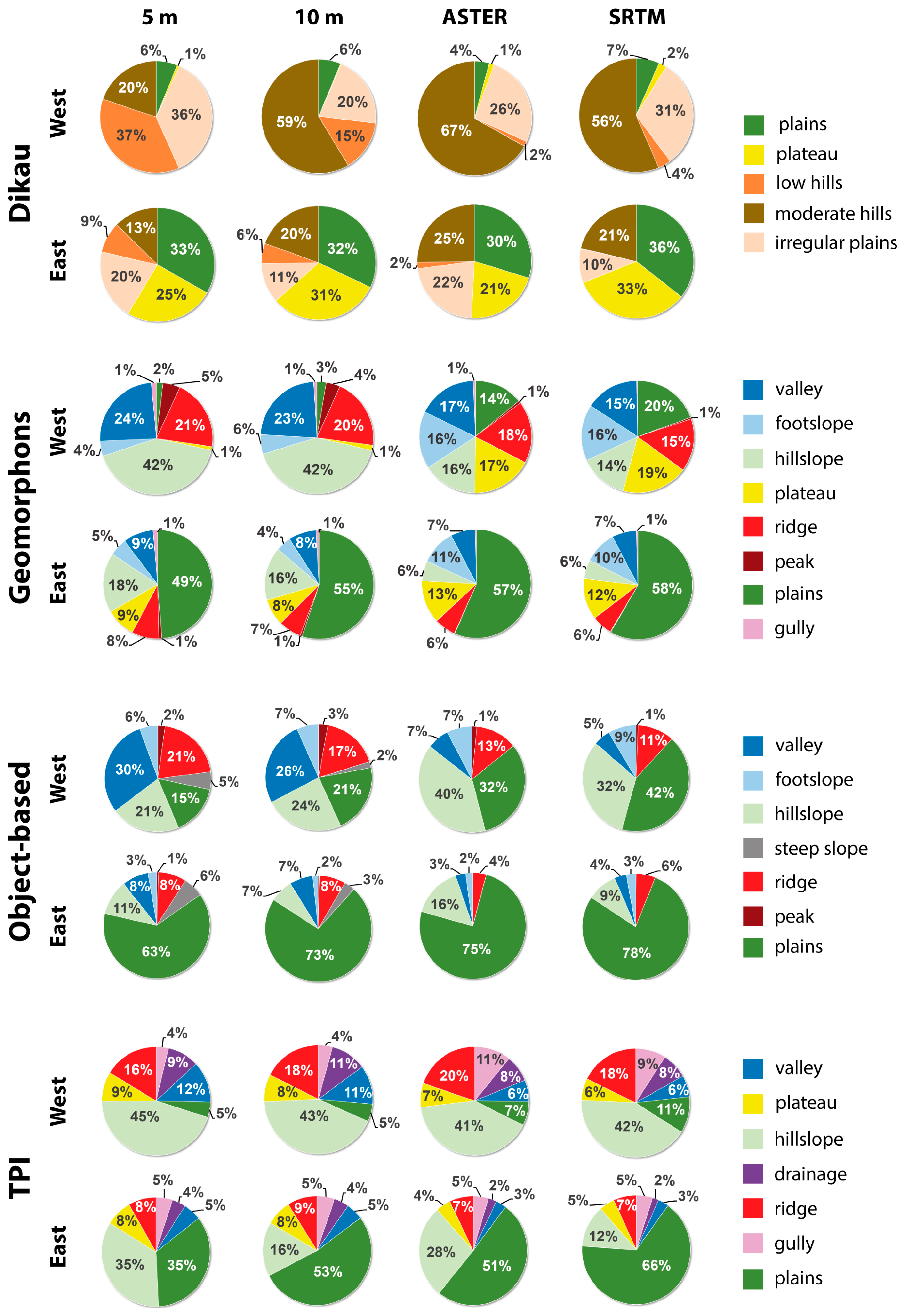
4.2. Classification Results

Figure 3 presents the percentage of the classified area for each landform class. All approaches indicate significant differences between the western and eastern study areas. Generally, they show more flat terrain in the eastern area, whereas the western area is dominated by landform classes that represent hilly landforms. Therefore, in the eastern site, the flat landscape representing the classes plains and plateau have the highest percentages and more than half of the pixels were classified by these classes. However, considerable differences between all approaches exist. While the proportion of the class plains with approximately 30% is relatively low for Dikau’s scheme, up to three-fourths of the pixels were classified as plains by the object based approach. In contrast, in the western study area, less than 20% were classified as flat areas in high geometric resolution datasets. There, only 15% were classified as plains by the object based approach and less than 6% by the others. The proportion of this class is largely stable in all spatial resolutions for Dikau’s approach, whereby it is strongly increasing for all other approaches in low resolution.

In the western study area, the majority of pixels were classified into landform classes that represent hilly areas or incised valley landforms. Over one-fourth of the pixels were classified as valleys, gullies or drainage by all approaches in high spatial resolution datasets. In Dikau’s approach the class irregular plains is the best suitable class for valleys. By this approach, 36% were classified as irregular plains, which is the highest rate for incised landforms compared to the other approaches. The results in low pixel resolution reveal a strong decrease of classified valleys for the object-based approach. Only 5% and 7% were classified as valleys with ASTER and SRTM DEM, respectively. For all other approaches, there is only a slight decrease of percentages. In the eastern study area, the percentages of valleys are slightly lower than in the western site. Apart from that, the results show the same properties in both sites.

Hills are the predominant landforms of the western study area. Therefore, all approaches classified the majority of pixels correctly into landforms, which represent hilly landforms. The percentage of these landforms with around 73% is the highest for geomorphons with a high geometric resolution DEM. The other approaches classify between 55% and 61% as hills. Most of these areas were classified as low and moderate hills by Dikau’s scheme and as hillslopes by the others. The percentage of hillslope with around 42–45% is relatively high for geomorphons and TPI, whereas only an area of just over 20% was classified with this landform class by the object based approach in high spatial resolution. However, in low spatial resolution, the percentage of hillslope pixels is strongly increasing for the object-based approach, whereas it decreases for the geomorphons approach. By Dikau’s approach, the majority was classified with the class low hills in the western area with a pixel resolution of 5 m. With low pixel resolutions, a significant increase of the percentage of the class moderate hills can be observed, whereas the class low hills is almost completely missing. The percentage of uprising landforms is significantly lower in the eastern study area. There, only 20–30% were classified as hilly landforms. Only the TPI shows for the results of 5 m and ASTER a higher proportion of 43% and 35%, respectively. This is mainly due to a disproportionately high rate of hillslope landforms.

In Figure 4, an exemplary section of the classified landform maps of the eastern classification result is illustrated. It compares the results of the four approaches with the different DEMs. Some differences in the relief subdivision are noticeable. Generally, the approach after Dikau shows the least relief differentiation. All other approaches have more classes to subdivide the relief, whereby a more detailed classification result can be achieved. In particular, the TPI and the geomorphons classify the landscape in a line-like way, which accents the structure of the landscape best. For the object-based approach, the results reveal for the strongly fragmented parts of the landscape some weaknesses of the segmentation technique. Some segments seem to be too big, which leads to a less accurately classification of the landforms in some areas.

A comparison of the different geometric resolutions reveals for all approaches the weakest results for both 30 m classifications. Compared to the results with high pixel resolution it is apparent that the landforms are classified spatially less accurately and small structures of the landscape were not detected. In contrast, the classification results with a pixel resolution of 5 m and 10 m show a much more differentiated subdivision of the landscape. Besides, they are less different from each other for three of the four approaches. Only for Dikau’s approach, significant changes in the results can be observed between all spatial resolution levels.

The classified landscape can be divided into three general landform elements: Flat areas, valleys and hills. The results of all approaches are compared in the following in detail for these areas.

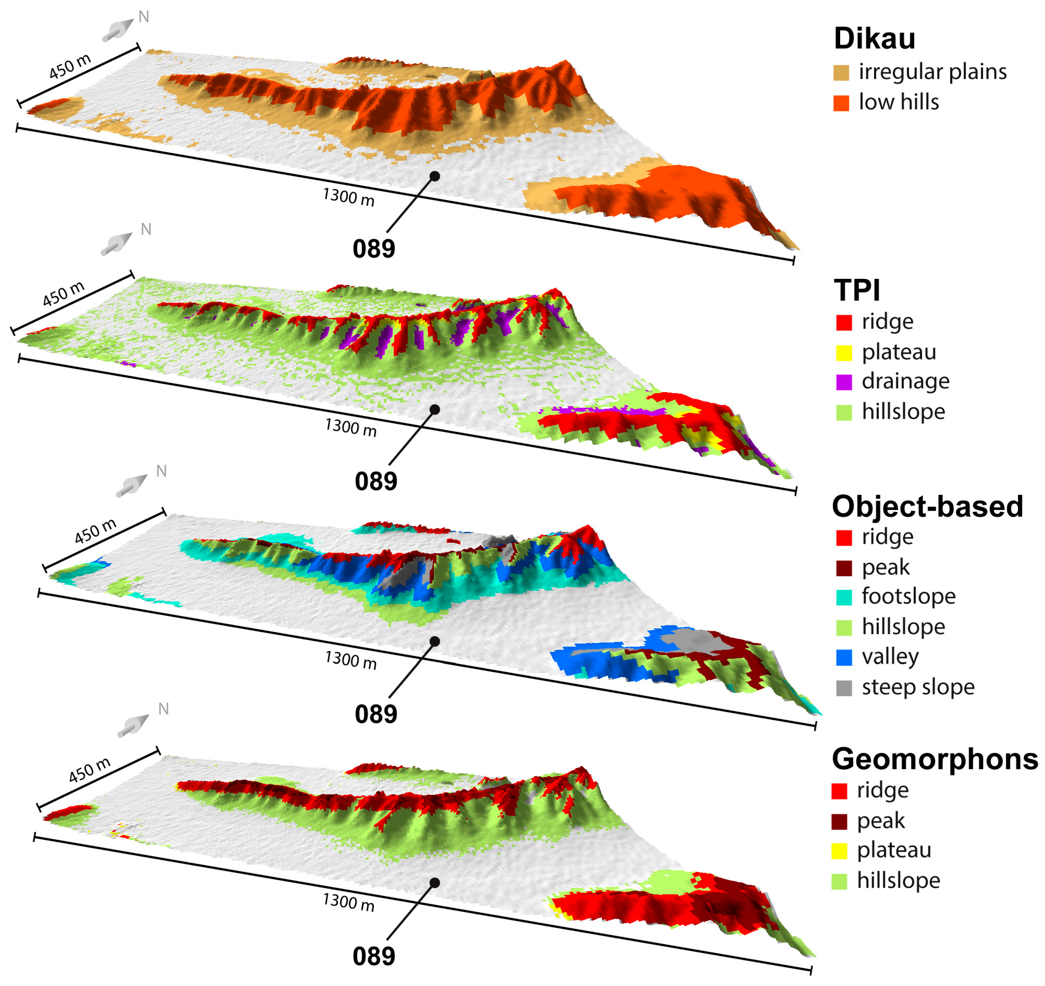
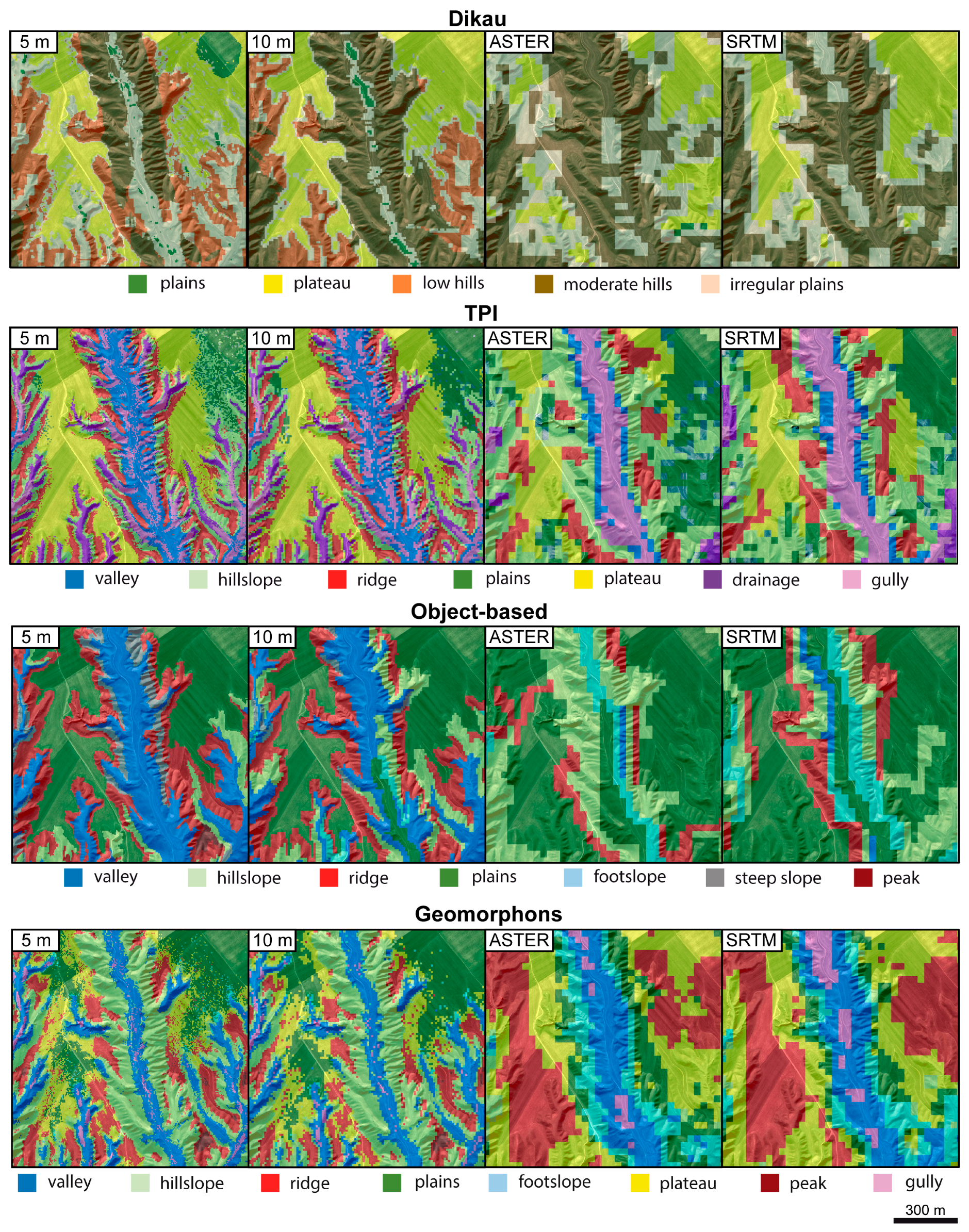
• Flat areas: With the highest spatial resolution DEM, the TPI approach yielded the weakest results for flat areas in both regions due to a very inhomogeneous classification with the classes plains and hillslope. The best results here can be observed by the object-based approach. Especially the segmentation technique leads to a very homogenous classification in wider areas. The geomorphons approach also produces relative homogenous results, but only in very large flat areas, as they exist in the Eastern study area. If the flat area is relatively small, the results demonstrate many misclassifications with the class footslope. Contrary to that, Dikau’s approach seems to be the best to classify small flat areas. Here the results of the Western study area show very homogenous and spatially accurate results, whereas in wider areas many mixtures with the class plateau can be observed.
• Valleys: All results reveal that small valleys only were classified with spatially high-resolution DEMs. With both 30 m terrain models only the most distinct valleys were detected by all classification methods. The approach of Dikau classifies them barely even with a pixel resolution of 10 m. Only with a pixel resolution of 5 m this approach is able to classify valleys with the landform class irregular plains. With lower pixel resolutions, this approach is hardly able to detect them. Generally, the results of the TPI have the most diversification in the classification of valleys, caused by the largest variety of classes to divide these landform elements. Therefore, the TPI is the only approach that can distinguish different valley types and assign them to different classes. An observable weakness of this approach is that valleys were classified too broadly and some areas of the neighboring hills were also classified as valleys (see Figure 4). It is also noticeable for this approach that both 30 m results classified the majority of valleys with the class gully, while they were assigned to the class valley in spatially high-resolution results. The weakness of too wide classified areas of the class valley can also be observed in the results of the object-based approach. Furthermore, the built segments seem to be spatially inaccurate in some places. In contrast, the most accurate classification of valley widths was achieved by the geomorphons approach with a high pixel resolution DEM. Furthermore, small incisions can be shown separately with the class gully by this approach. However, the general subdivision of different incision types is less differentiated than by the TPI.
• Hills: A comparison of the classification results of hilly landforms indicates the least differentiation of the relief with Dikau’s approach, caused by the fact that it just classifies these areas with the classes low hills and moderate hills. Furthermore, the results of Dikau’s classification show a systematic change in the amount of classified landforms with the class low hills. Whereby with a pixel resolution of 5 m the lower hills of the western part of the plateau were assigned correctly as low hills, with both 30 m DEMs almost all hills were classified as moderate hills. All other approaches produce much more diversity in their results, because their classification scheme is able to subdivide the hills into smaller sub elements. Figure 5 depicts the classification schemes of the four approaches in spatially high-resolution on a typical range of hills in the western study area. In particular, the object-based approach has many suitable classes for a systematic classification of hills. However, the results reveal that the extremely fragmented structure of the hills is often not depicted accurate enough by the segments. Therefore, many classified landforms do not fit properly to the relief and overlap with areas, which should be better classified with another landform class. This leads to the effect that the classification result of the object-based approach seems to be coarser than the results of the TPI and geomorphons approach. A specific feature of the object-based approach is the differentiation between different slope gradients by the classes steep slope and hillslope. The results demonstrate that the subdivision works properly only with a spatially high-resolution DEM. It is observed that the amount of classified steep slope areas decreases strongly for lower pixel resolutions. With a geometric resolution of 30 m nearly no steep slope landforms were detected. The geomorphons approach generally classifies hills with the classes hillslope and the upper parts with the classes ridge and peak. Noticeable is that lower parts were not classified with the class footslope in the results with high pixel resolutions, although this class would be more suitable. A comparison of high and low resolution results reveals a changed system in the classification of hillsides. Whereas the slopes were assigned to the class hillslope in spatially high-resolution results, most areas were classified with the classes footslope and plateau with a low pixel resolution DEM. Furthermore, it is conspicuous that the classified landforms are much coarser with both 30 m DEMs.

The spatially high-resolution results of the TPI generally point out a largely reasonable and accurate landform classification of hills. It has minor class diversity from the geomorphons and object-based approach, but especially the classification of hillslope and ridges is highly consistent and accurate. Only the classification of some upper parts of the hills with the class plateau in the western study area seems not meaningful. It seems that this class classifies different landform types in the eastern, but not in the western area. Therefore, the class name here is only suitable for the eastern part.

4.3. Accuracy Assessment

The final classification results were compared with landforms depicted in 66 pictures from both areas.

Table 7. Overall accuracy of the four approaches and the four different datasets derived as the relation of correctly classified to all classified elements from the confusion matrices (Table A1, Table A2, Table A3 and Table A4).

	5 m	10 m	Aster 30 m	SRTM 30 m
Dikau	63%	58%	33%	42%
TPI	72%	71%	44%	41%
Object-based	63%	63%	42%	40%
Geomorphons	70%	65%	39%	39%

gives an overview of all achieved overall accuracies. The results show as expected a minor accuracy for the DEM with a pixel resolution of 30 m. The variation of the results is higher for the ASTER dataset than for the SRTM dataset. This is mainly due to the very low accuracy of Dikau’s approach for this specific area. The higher pixel resolution of the Pléiades dataset results in an increase of 20–30% of the classification accuracy. In addition, the differences in the accuracy between the 5 m and 10 m pixel resolution results are very low. Especially the TPI and the object-based approach achieve nearly the same accuracies in both spatial resolutions. Generally, the accuracy of the TPI approach is the best, followed by the geomorphons approach. The approach of Dikau generated the lowest accuracy, except for the SRTM dataset.

The error matrices of the four approaches, as listed in

Table A1. Error matrix based on classified landform units for Dikau’s approach for the four different DEMs (5 = 5 m, 10 = 10 m, A = Aster 30 m, S = SRTM 30 m) with producer’s accuracy (PA) and user’s accuracy (UA).

		Reference Data
Classification	Landform Class	Plains				Plateau				Irregular Plains				Low Hills				Moderate Hills				Total				UA (%)
		5	10	A	S	5	10	A	S	5	10	A	S	5	10	A	S	5	10	A	S	5	10	A	S	5	10	A	S
	plains	11	11	5	9	1	2	3	3	2	3	5	7	0	0	0	2	0	0	0	0	14	16	13	21	79	69	38	43
	plateau	3	3	0	0	4	3	2	2	0	1	0	0	0	0	0	1	0	0	0	1	7	7	2	4	57	43	100	50
	irregular plains	9	6	8	6	2	1	2	2	18	13	9	13	3	4	4	6	0	0	7	8	32	24	30	35	56	54	30	37
	low hills	0	0	0	0	0	0	0	0	0	0	0	0	15	11	0	1	9	1	0	0	24	12	0	1	63	92	-	100
	moderate hills	1	1	5	2	0	2	2	1	3	9	12	5	4	8	16	13	16	18	16	16	24	38	51	37	67	47	31	43
	Total	24	21	18	17	7	8	9	8	23	26	26	25	22	23	20	23	25	19	23	25	101	97	96	98
	PA (%)	46	52	28	53	57	38	22	25	78	50	35	52	68	48	0	4	64	95	70	64

,

Table A2. Error matrix based on classified landform units for the TPI approach for the four different DEMs (5 = 5 m, 10 = 10 m, A = Aster 30 m, S = SRTM 30 m) with producer’s accuracy (PA) and user’s accuracy (UA).

		Reference Data
Classification	Landform Class	Gully				Drainage				Valley				Plains				Hillslope				Plateau				Ridge				Total				UA (%)
		5	10	A	S	5	10	A	S	5	10	A	S	5	10	A	S	5	10	A	S	5	10	A	S	5	10	A	S	5	10	A	S	5	10	A	S
	gully	13	12	9	9	2	1	2	2	4	3	12	12	0	1	5	3	3	1	5	4	0	0	1	1	0	0	3	1	22	18	37	32	59	67	24	28
	drainage	1	1	1	1	9	8	1	1	1	0	2	1	1	0	2	3	4	3	2	1	0	0	0	0	0	0	0	0	16	12	8	7	56	67	13	14
	valley	3	2	2	2	0	0	0	0	13	12	2	2	10	8	2	6	6	8	3	3	0	0	0	0	2	1	3	4	34	31	12	17	38	39	17	12
	plains	0	0	1	1	0	0	0	0	2	1	1	1	11	12	8	8	1	1	1	3	0	0	0	0	0	0	1	3	14	14	12	16	79	86	67	50
	hillslope	0	0	1	0	0	0	3	4	1	0	0	0	3	4	3	2	24	18	15	14	2	2	2	2	0	3	10	10	30	27	34	32	80	67	44	44
	plateau	0	0	0	0	0	0	1	2	0	0	0	0	0	0	0	0	1	2	2	3	7	5	3	3	0	0	1	4	8	7	7	12	88	71	43	25
	ridge	0	0	0	0	0	0	3	2	0	0	0	0	0	0	1	0	1	0	2	2	0	1	1	1	47	38	23	21	48	39	30	26	98	97	77	81
	Total	17	15	14	13	11	9	10	11	21	16	17	16	25	25	21	22	40	33	30	30	9	8	7	7	49	42	41	43	172	148	140	142
	PA (%)	76	80	64	69	82	89	10	9	62	75	12	13	44	48	38	36	60	55	50	47	78	63	43	43	96	90	56	49

,

Table A3. Error matrix based on classified landform units for the object-based approach for the four different DEMs (5 = 5 m, 10 = 10 m, A = Aster 30 m, S = SRTM 30 m) with producer’s accuracy (PA) and user’s accuracy (UA).

		Reference Data
Classification	Landform Class	Peak				Ridge				Steep Slope				Plains				Hillslope				Valley				Footslope				Total				UA (%)
		5	10	A	S	5	10	A	S	5	10	A	S	5	10	A	S	5	10	A	S	5	10	A	S	5	10	A	S	5	10	A	S	5	10	A	S
	peak	5	6	4	0	5	4	0	0	0	0	0	0	0	0	0	0	0	0	1	0	0	0	0	0	0	0	0	0	10	10	5	0	50	60	80	-
	ridge	7	6	8	8	21	21	13	10	0	1	1	4	0	0	0	0	3	4	3	1	0	0	2	0	0	0	1	0	31	32	28	23	68	66	46	43
	steep slope	0	0	0	0	0	0	0	0	6	5	0	0	0	0	0	0	4	3	0	0	0	0	0	0	0	0	0	0	10	8	0	0	60	63	-	-
	plains	0	0	0	1	0	0	7	8	0	0	0	0	22	23	17	25	0	0	5	11	2	4	2	12	0	0	2	3	24	27	33	60	92	85	52	42
	hillslope	0	0	0	1	3	2	8	10	3	3	7	3	2	0	10	1	11	13	12	12	3	0	8	2	0	1	2	3	22	19	47	32	50	68	26	38
	valley	0	0	0	0	2	1	0	0	0	0	0	3	2	1	3	1	10	12	2	3	18	18	12	7	3	3	1	0	35	35	18	14	51	51	67	50
	footslope	0	0	0	0	1	1	1	0	0	1	1	1	2	3	2	1	1	0	5	3	2	4	4	4	9	7	4	3	15	16	17	12	60	44	24	25
	Total	12	12	12	10	32	29	29	28	9	10	9	11	28	27	32	28	29	32	28	30	25	26	28	25	12	11	10	9	147	147	148	141
	PA (%)	42	50	33	0	66	72	45	36	67	50	0	0	79	85	53	89	38	41	43	40	72	69	43	28	75	64	40	33

and

Table A4. Error matrix based on classified landform units for the geomorphons approach for the four different DEMs (5 = 5 m, 10 = 10 m, A = Aster 30 m, S = SRTM 30 m) with producer’s accuracy (PA) and user’s accuracy (UA).

		Reference Data
Classification	Landform Class	Plains				Peak				Ridge				Plateau				Hillslope				Footslope				Valley				Gully				Total				UA (%)
		5	10	A	S	5	10	A	S	5	10	A	S	5	10	A	S	5	10	A	S	5	10	A	S	5	10	A	S	5	10	A	S	5	10	A	S	5	10	A	S
	plains	9	7	4	5	0	0	0	0	0	0	1	1	0	0	0	1	0	0	2	3	0	0	0	0	0	0	0	1	0	0	0	0	9	7	7	11	100	100	57	45
	peak	0	0	0	0	8	8	1	1	6	7	0	0	0	0	0	0	0	0	1	0	0	0	0	0	0	0	0	0	0	0	0	0	14	15	2	1	57	53	50	100
	ridge	1	1	0	0	2	1	4	6	24	19	13	9	0	1	1	1	4	6	3	2	0	0	0	0	0	0	2	0	0	0	0	0	31	28	23	18	77	68	57	50
	plateau	0	0	0	0	0	0	1	0	0	0	3	8	3	2	3	1	0	0	6	6	0	0	0	0	0	0	2	1	0	0	0	0	3	2	15	16	100	100	20	6
	hillslope	4	3	1	0	0	0	0	0	3	3	3	2	2	0	0	1	23	20	5	9	2	3	1	0	0	1	0	0	0	0	0	0	34	30	10	12	68	67	50	75
	footslope	6	5	7	7	0	0	1	1	0	0	3	2	0	0	1	1	0	2	6	5	5	2	6	6	2	0	7	8	0	0	0	0	13	9	31	30	38	22	19	20
	valley	3	8	8	8	0	0	2	1	1	1	2	5	0	1	2	0	5	1	5	4	0	0	0	0	30	31	24	24	3	5	8	8	42	47	51	50	71	66	47	48
	gully	0	0	0	1	0	0	0	0	0	0	1	0	0	0	0	0	0	0	1	0	0	0	0	0	6	3	4	3	12	9	1	0	18	12	7	4	67	75	14	0
	Total	23	24	20	21	10	9	9	9	34	30	26	27	5	4	7	5	32	29	29	29	7	5	7	6	38	35	39	37	15	14	9	8	164	150	146	142
	PA (%)	39	29	20	24	80	89	11	11	71	63	50	33	60	50	43	20	72	69	17	31	71	40	86	100	79	89	62	65	80	64	11	0

, generally underline the presented results. For the datasets with a lower spatial resolution, the accuracy decreases by about 20% to 30%. For Dikau’s scheme (Table A1), the user’s accuracy is decreasing on lower pixel resolutions and SRTM shows slightly better results than the ASTER based classification. Plains and low hills are best classified. Likewise, the producer’s accuracy points out a decrease to lower pixel resolutions and the classes of irregular plains, low hills, and moderate hills show the best fit. In particular, irregular plains and moderate hills are mixed.

For the TPI approach (Table A2), the results of the spatially high-resolution Pleiades DEMs produced low user’s accuracies for the class of valleys, due to their strong mixture with other flat areas. For the other classes the majority of ground truth landforms were identified correctly by the TPI approach. Similar to the other approaches the accuracies decrease strongly for both 30 m datasets for most classes.

The results of the object-based classification (Table A3) indicate generally more stable results over all geometric resolutions. In particular, plains were classified very well in the datasets with 5 m and 10 m pixel resolution. In contrast, in the classification results of the ASTER and SRTM dataset all steep slope landforms were classified into other landforms and the class was not used at all. Similar results can be recognized for the class peak, which was also classified rarely for 30 m pixel resolution datasets. Although the class was relatively often misclassified into the class ridge, the accuracies are generally low. Noticeable is also a strong increase of the amount of classified landforms with the classes plains and hillslope in both 30 m datasets, due to misclassifications of other landforms into these classes.

The error matrix of the geomorphons approach in Table A4 shows a general decline of the user’s accuracy with both 30 m datasets. The decline between 5 m and 10 m is very small. The classification of the class footslope works less and was mixed with classifications of plains and valleys mostly. Interestingly, the accuracy rises for the classes of peaks and hillslopes.

5. Discussion

A comparison of the different landform classification results reveals strengths and weaknesses for all approaches. Overall, the TPI and the geomorphons approach achieved the highest accuracies. In addition, their classification results give the best visual feedback of the landscape structure of the Iranian loess plateau due to their spatially accurate classification of landforms. In particular, the TPI seems most suitable for a meaningful classification, as it has the highest class diversity for the classification of hills, hillslopes and valleys. However, it revealed some weaknesses in flat landscapes due to a very inhomogeneous classification of these areas with high pixel resolution datasets. In contrast, the geomorphons approach achieves higher accuracies in the classification of plains and valleys. However, it classifies the structures of hilly landforms less detailed compared to the TPI, although the number of suitable classes is similar. Nonetheless, both approaches seem to have the highest suitability to classify such a distinct relief at this scale.

In this study, Dikau’s approach achieved the lowest accuracies. Moreover, the classification results reveal the least relief differentiation compared to the other approaches. Overall, this approach seems to be least suitable for the classification of such a strongly dissected landscape. Due to its possible landform classes, it is probably more appropriate for the classification of landforms in other spatial scales. In addition, many authors demonstrated in their work a better suitability of the Dikau approach for landscapes on macroscales [11,49,50,51].

The object based classification produced ambivalent results. The advances of the segmentation technique can only be confirmed here for landforms, which extend over larger areas. Especially flat areas were classified best by this approach because of a high degree of homogeneity. In contrast, weaknesses by the classification of smaller landforms are recognizable in parts with rougher relief. Mainly this is the result of a minor spatial accuracy of the built segments in those areas. As a result, the classified landform boundaries are spatially less accurate compared to the applied pixel based approaches. A more complex segmentation process on different scales would probably avoid this problem. For example, a segmentation on different scale levels as postulated by Drǎguţ and Eisank [28] accounts the issue of under-segmentation of small objects or over-segmentation of the larger ones.

A comparison of the results in different spatial resolutions clearly demonstrates poor results for all approaches with both 30 m DEMs. Small landforms were not detected and the spatial accuracy of landform borders is less accurate. Only in extensive flat areas of the eastern part, a lower pixel resolution appears to result in a more homogenous classification compared to the high-resolution results. However, differences between the ASTER and the SRTM DEMs are recognizable. Generally, a higher suitability of the SRTM dataset for landform classifications was postulated by several authors [52,53,54]. This can be confirmed here as the use of the SRTM DEM results into a more homogeneous landform classification.

Nevertheless, both datasets are not able to achieve promising results in the majority of evaluated areas in this contribution. This is basically due to two main reasons. One reason lies in the DEM itself as the strongly dissected relief structure is already insufficiently contained in the input dataset. Generally, lower spatial resolutions lead to a smoother representation of the topography and the relief seems in the DEM much gentler and more rounded as it is in reality [31]. Therefore, neither the ASTER GDEM nor the SRTM dataset include enough information to classify the very small landscape structures.

The second reason lies in the characteristic of the moving windows, which were used by most approaches in some way to classify landforms. The moving window defines the number of surrounding pixels, which were included into the classification process to classify a certain pixel. A suitable definition is difficult due to different landscape characteristics and landform sizes. In the ideal case, it contains only landscape elements which directly affect the landform of the considered pixel. Bigger window sizes result in too many considered pixels by the classification processes, which have no influence on the considered landform. Thus, the choice of the best possible window size depends strongly on the scale of landforms and uneven landscapes mostly require smaller window sizes to represent small features [21,22]. Due to the very small landform elements in the study area it was necessary for Dikau’s approach to define a very small 3 × 3 pixel window already for the 5 m pixel resolution DEM. Thus, a further reduction of contemplated pixels was not possible for lower resolutions, which leads to an enlargement of the window size. The TPI and geomorphons approaches were affected by the same problem as the minimum window size was reached with a 10 m DEM. As a result, the window size also gets too big with a 30 m pixel resolution DEM. In consequence, small landforms were not classified and bigger landforms were interpreted in false dimensions and assigned to incorrect classes. This effect is clearly recognizable in the results of the TPI where landforms, which were classified as valleys with a high-pixel resolution DEM, were assigned to class gully in lower resolutions. Hence, a differentiation between gullies and valleys was not possible. In addition, the amount of classified peaks decreases significantly in lower resolutions in the results of the geomorphons approach.

The results clearly point out that a geometric resolution of at least 10 m is necessary for an accurate classification of such a strongly dissected relief. With both 30 m DEMs, no approaches are able to achieve sufficient results. A comparison of the classification results of the western and eastern study area indicate that flatter areas are less sensitive to resolution changes. Furthermore, low spatial resolutions lead to an increase of homogeneity. Thus, it can be confirmed here that the flatter the landscape is, the lower the spatial DEM resolution can be to achieve accurate classification results. In this contribution, the best results were achieved with a pixel resolution of 5 m. For such a strongly varying landscape also a higher pixel resolution of around 3 m would probably effectuate results of similar quality, but higher pixel resolutions increase the risk of an over-classification of landforms. With a decreasing pixel size, too many micro-scaled landforms were identified, which were not necessary for further landscape interpretations [55].

The accuracy assessment method conducted in this contribution provides reproducible results. However, a quantitative evaluation of landform classifications is still problematic. First, the acquisition of ground truth data is often time consuming and depends on the suitability of the terrain [23,56]. Second, in this contribution, a relatively high number of photos were required to collect enough ground truth data for all classes to produce a statistically valid dataset. Furthermore, weaknesses still exist in the evaluation methodology itself. Several studies have shown that an accuracy assessment with ground truth based error matrices is able to produce suitable results for geomorphometric classifications. However, a quantitative accuracy assessment of landform classifications is problematic as there still exists a lack of standardized applicable methods. Several authors have found different solutions to extract their ground truth data and to compare them with their results. Some studies interpreted landforms from aerial or ground taken photos and generated ground truth samples to conduct an evaluation landform. Schneevoigt et al. [27] also defined test areas for each landform from photo material but evaluated them pixel-based. Others generated a reference map from map data or field investigations and compared it pixel-wise to their results [24,57].

A pixel-wise comparison seemed unsuitable in this study, as this would have overrepresented some landforms due to their spatial extent. Landforms vary strongly in their extent, as there exist point-based, line-based and areal landforms [58]. Consequently, in a pixel-wise evaluation the class plains, as an areal landform, would have contained much more pixels in the error matrix than the class peak as a point based landform. This would have led to a significant overrepresentation of some landforms in a pixel-wise evaluation process. Therefore, a landform-wise comparison method was applied here to avoid the influence of the spatial extent of landforms. In addition, the comparison is not biased by positional errors of the input datasets or the varying notation and detail of the applied approaches.

A major problem in geomorphometric analyses is that a clear delimitation of landforms is often not possible, as they do not have distinct boundaries [23,58]. Hence, the interpretation of these landforms is rather subjective. Moreover, a standardization of the classes between the different approaches was not completely possible in this contribution due to diverse creation processes of the different approaches. Landform classes with the same name potentially do not exactly represent the same real landform, what makes them not completely comparable. In consequence, a high effort and dependency on the knowledge of the interpreter is still necessary in the interpretation and delineation of landforms. Furthermore, some influence of subjectivity on the evaluation process cannot be prevented.

6. Conclusions

Landform classifications can be derived by a high diversity of possible input data, different approaches and result in a multiplicity of landform classes. In this contribution, a comparison of four prominent approaches was conducted with four input datasets with different spatial resolutions and different measurement methods. The results show for the selected areas of the Iranian loess plateau, which is highly dissected that higher resolution datasets are necessary to achieve satisfying overall accuracies. With the 5 m Pleiades DEM the TPI and geomorphons approach achieved accuracies of greater than 70% and the two other approaches reached overall accuracies of greater than 60%. SRTM data worked generally better than ASTER GDEM data, but both elevation models are not able to generate accurate classification results here and only achieved accuracies of about 40%. Thus, a decrease of 20%–30% for the lower spatial resolution datasets is detected. This variety in accuracy needs to be regarded before applying the derived landforms for further calculations. We expect that the applied methodological approach will lead to similar results concerning the accuracy of landform classifications if applied to other areas with similar landform characteristics. As shown here, differences between the approaches and resolutions are smaller for areas with more flat terrain. All selected approaches show weaknesses; in this case, the TPI and geomorphons approach revealed the best results and are more detailed in terms of derivable landform types. The approach of Dikau is generally less suitable for these areas and the approach based on the object segmentation is less accurate for areas with a rougher relief. However, the selection of moving window size and the accurate derivation of objects influences the results. The accuracy assessment of these classifications and the delineation between different landforms is influenced by the user.

References

- Pike, R.J.; Park, M. Geomorphometry—Progress, practice and prospect. Z. Geomorphol. 1995, 101, 221–235. [Google Scholar]
- Florinsky, I. Digital Terrain Analysis in Soil Science and Geology; Academic Press: Amsterdam, The Netherlands, 2011. [Google Scholar]
- Behrens, T.; Zhu, A.X.; Schmidt, K.; Scholten, T. Multi-scale digital terrain analysis and feature selection for digital soil mapping. Geoderma 2010, 155, 175–185. [Google Scholar] [CrossRef]
- Behrens, T.; Schmidt, K.; Ramirez-Lopez, L.; Gallant, J.; Zhu, A.X.; Scholten, T. Hyper-scale digital soil mapping and soil formation analysis. Geoderma 2014, 213, 578–588. [Google Scholar] [CrossRef]
- Bishop, M.P.; James, L.A.; Shroder, J.F.; Walsh, S.J. Geospatial technologies and digital geomorphological mapping: Concepts, issues and research. Geomorphology 2012, 137, 5–26. [Google Scholar] [CrossRef]
- Armstrong, R.N.; Martz, L.W. Topographic parameterization in continental hydrology: A study in scale. Hydrol. Process. 2003, 17, 3763–3781. [Google Scholar] [CrossRef]
- Schwanghart, W.; Groom, G.; Kuhn, N.J.; Heckrath, G. Flow network derivation from a high resolution DEM in a low relief, agrarian landscape. Earth Surf. Process. Landf. 2013, 38, 1576–1586. [Google Scholar] [CrossRef]
- Barka, I.; Vladovic, J.; Máli, Š. Landform Classification and Its Application in Predictive Mapping of Soil and Forest Units. In Proceedings of the GIS Ostrava, Ostrava, Czech Republic, 24–26 January 2011; p. 11. [Google Scholar]
- Wood, S.W.; Murphy, B.P.; Bowman, D.M.J.S. Firescape ecology: How topography determines the contrasting distribution of fire and rain forest in the south-west of the Tasmanian Wilderness World Heritage Area. J. Biogeogr. 2011, 38, 1807–1820. [Google Scholar] [CrossRef]
- Pennock, D.J.; Zebarth, B.J.; De Jong, E. Landform classification and soil distribution in hummocky terrain, Saskatchewan, Canada. Geoderma 1987, 40, 297–315. [Google Scholar] [CrossRef]
- Dikau, R.; Brabb, E.; Mark, R.K.; Pike, R.J. Morphometric landform analysis of New Mexico. Z. Geomorphol. Suppl. 1995, 101, 109–126. [Google Scholar]
- Hammond, E.H. Small-Scale Continental Landform Maps. Ann. Assoc. Am. Geogr. 1954, 44, 33–42. [Google Scholar] [CrossRef]
- Hammond, E.H. Analysis of Properties in Land Form Geography: An Application to Broad-Scale Land Form Mapping. Ann. Assoc. Am. Geogr. 1964, 54, 11–19. [Google Scholar] [CrossRef]
- Brabyn, L. GIS Analysis of Macro Landform. In Proceedings of the 10th Colloquium of the Spatial Information Research Centre, Dunedin, New Zealand, 16–19 November 1998; pp. 35–48. [Google Scholar]
- MacMillan, R.A.; Pettapiece, W.W.; Nolan, S.C.; Goddard, T.W. A generic procedure for automatically segmenting landforms into landform elements using DEMs, heuristic rules and fuzzy logic. Fuzzy Sets Syst. 2000, 113, 81–109. [Google Scholar] [CrossRef]
- Iwahashi, J.; Pike, R.J. Automated classifications of topography from DEMs by an unsupervised nested-means algorithm and a three-part geometric signature. Geomorphology 2007, 86, 409–440. [Google Scholar] [CrossRef]
- Klingseisen, B.; Metternicht, G.; Paulus, G. Geomorphometric landscape analysis using a semi-automated GIS-approach. Environ. Model. Softw. 2008, 23, 109–121. [Google Scholar] [CrossRef]
- Burrough, P.A.; Van Gaans, P.F.M.; MacMillan, R.A. High-resolution landform classification using fuzzy k-means. Fuzzy Sets Syst. 2000, 113, 37–52. [Google Scholar] [CrossRef]
- Schmidt, J.; Hewitt, A. Fuzzy land element classification from DTMs based on geometry and terrain position. Geoderma 2004, 121, 243–256. [Google Scholar] [CrossRef]
- Weiss, A.D. Topographic position and landforms analysis. In Proceedings of the ESRI User Conference, San Diego, CA, USA, 9–13 July 2001. [Google Scholar]
- De Reu, J.; Bourgeois, J.; Bats, M.; Zwertvaegher, A.; Gelorini, V.; De Smedt, P.; Chu, W.; Antrop, M.; De Maeyer, P.; Finke, P.; et al. Application of the topographic position index to heterogeneous landscapes. Geomorphology 2013, 186, 39–49. [Google Scholar] [CrossRef]
- Jasiewicz, J.; Stepinski, T.F. Geomorphons—A pattern recognition approach to classification and mapping of landforms. Geomorphology 2013, 182, 147–156. [Google Scholar] [CrossRef]
- Drǎguţ, L.; Blaschke, T. Automated classification of landform elements using object-based image analysis. Geomorphology 2006, 81, 330–344. [Google Scholar] [CrossRef]
- Pedersen, G.B.M. Semi-automatic classification of glaciovolcanic landforms: An object-based mapping approach based on geomorphometry. J. Volcanol. Geotherm. Res. 2016, 311, 29–40. [Google Scholar] [CrossRef]
- Van Asselen, S.; Seijmonsbergen, A.C. Expert-driven semi-automated geomorphological mapping for a mountainous area using a laser DTM. Geomorphology 2006, 78, 309–320. [Google Scholar] [CrossRef]
- D’Oleire-Oltmanns, S.; Eisank, C.; Drǎgut, L.; Blaschke, T. An object-based workflow to extract landforms at multiple scales from two distinct data types. IEEE Geosci. Remote Sens. Lett. 2013, 10, 947–951. [Google Scholar] [CrossRef]
- Schneevoigt, N.J.; van der Linden, S.; Thamm, H.P.; Schrott, L. Detecting Alpine landforms from remotely sensed imagery. A pilot study in the Bavarian Alps. Geomorphology 2008, 93, 104–119. [Google Scholar] [CrossRef]
- Drǎguţ, L.; Eisank, C. Automated object-based classification of topography from SRTM data. Geomorphology 2012, 141–142, 21–33. [Google Scholar] [CrossRef] [PubMed]
- Dekavalla, M.; Argialas, D. Object-based classification of global undersea topography and geomorphological features from the SRTM30_PLUS data. Geomorphology 2017, 288, 66–82. [Google Scholar] [CrossRef]
- Camiz, S.; Poscolieri, M.; Roverato, M. Geomorphometric comparative analysis of Latin-American volcanoes. J. South Am. Earth Sci. 2017, 76, 47–62. [Google Scholar] [CrossRef]
- Deng, Y.; Wilson, J.P.; Bauer, B.O. DEM resolution dependencies of terrain attributes across a landscape. Int. J. Geogr. Inf. Sci. 2007, 21, 187–213. [Google Scholar] [CrossRef]
- Zhang, W.; Montgomery, D.R. Digital elevation model grid size, landscape representation, and hydrologic simulations. Water Resour. Res. 1994, 30, 1019–1028. [Google Scholar] [CrossRef]
- Kienzle, S. The Effect of DEM Raster Resolution on First Order, Second Order and Compound Terrain Derivatives. Trans. GIS 2004, 8, 83–111. [Google Scholar] [CrossRef]
- Zink, M.; Bachmann, M.; Brautigam, B.; Fritz, T.; Hajnsek, I.; Moreira, A.; Wessel, B.; Krieger, G. TanDEM-X: The New Global DEM Takes Shape. IEEE Geosci. Remote Sens. Mag. 2014, 2, 8–23. [Google Scholar] [CrossRef]
- Frechen, M.; Kehl, M.; Rolf, C.; Sarvati, R.; Skowronek, A. Loess chronology of the Caspian Lowland in Northern Iran. Quat. Int. 2009, 198, 220–233. [Google Scholar] [CrossRef]
- Khormali, F.; Kehl, M. Micromorphology and development of loess-derived surface and buried soils along a precipitation gradient in Northern Iran. Quat. Int. 2011, 234, 109–123. [Google Scholar] [CrossRef]
- Lauer, T.; Vlaminck, S.; Frechen, M.; Rolf, C.; Kehl, M.; Shari, J.; Lehndorff, E.; Khormali, F. The Agh Band loess-palaeosol sequence—A terrestrial archive for climatic shifts during the last and penultimate glacial–interglacial cycles in a semiarid region in Northern Iran. Quat. Int. 2017, 429, 13–30. [Google Scholar] [CrossRef]
- Kehl, M. Quaternary Loesses, Loess-Like Sediments, Soils and Climate Change in Iran; Gebrüder Borntraeger Verlagsbuchhandlung: Stuttgart, Germany, 2010. [Google Scholar]
- Bretis, B.; Grasemann, B.; Conradi, F. An active fault zone in the Western Kopeh Dagh (Iran). Austrian J. Earth Sci. 2012, 105, 95–107. [Google Scholar]
- Abrams, M. The Advanced Spaceborne Thermal Emission and Reflection Radiometer (ASTER): Data products for the high spatial resolution imager on NASA’s Terra platform. Int. J. Remote Sens. 2000, 21, 847–859. [Google Scholar] [CrossRef]
- Hirano, A.; Welch, R.; Lang, H. Mapping from ASTER stereo image data: DEM validation and accuracy assessment. ISPRS J. Photogramm. Remote Sens. 2003, 57, 356–370. [Google Scholar] [CrossRef]
- Tachikawa, T.; Kaku, M.; Iwasaki, A.; Gesch, D.B.; Oimoen, M.J.; Zhang, Z.; Danielson, J.J.; Krieger, T.; Curtis, B.; Haase, J.; et al. ASTER Global Digital Elevation Model Version 2—Summary of Validation Results, 2nd ed.; NASA: Washington, DC, USA, 2011.
- Abrams, M.; Tsu, H.; Hulley, G.; Iwao, K.; Pieri, D.; Cudahy, T.; Kargel, J. The Advanced Spaceborne Thermal Emission and Reflection Radiometer (ASTER) after fifteen years: Review of global products. Int. J. Appl. Earth Obs. Geoinf. 2015, 38, 292–301. [Google Scholar] [CrossRef]
- Farr, T.G.; Rosen, P.A.; Caro, E.; Crippen, R.; Duren, R.; Hensley, S.; Kobrick, M.; Paller, M.; Rodriguez, E.; Roth, L.; et al. The Shuttle Radar Topography Mission. Rev. Geophys. 2007, 45. [Google Scholar] [CrossRef]
- Astrium GEO-Information Services. Pléiades Imagery User Guide V 2.0; Astrium: Paris, France, 2012. [Google Scholar]
- De Lussy, F.; Kubik, P.; Greslou, D.; Pascal, V.; Gigord, P.; Cantou, J.P. Pleiades-HR image system products and quality Pleiades-HR image system products and geometric accuracy. In Proceedings of the ISPRS Hannover Workshop, Hannover, Germany, 17–20 May 2005. [Google Scholar]
- Gleyzes, M.A.; Perret, L.; Kubik, P. Pleiades system architecture and main performances. Int. Arch. Photogramm. Remote Sens. Spat. Inf. Sci. 2012, 39, 537–542. [Google Scholar] [CrossRef]
- Yokoyama, R.; Shlrasawa, M.; Pike, R.J. Visualizing Topography by Openness: A New Application of Image Processing to Digital Elevation Models. Photogramm. Eng. Remote Sens. 2002, 68, 257–265. [Google Scholar]
- Gallant, A.L.; Brown, D.D.; Hoffer, R.M. Automated mapping of Hammond’s landforms. IEEE Geosci. Remote Sens. Lett. 2005, 2, 384–388. [Google Scholar] [CrossRef]
- Hrvatin, M.; Perko, D. Suitability of Hammond’s Method for Determining Landform Units in Slovenia. Acta Geogr. Slov. 2009, 49, 343–366. [Google Scholar] [CrossRef]
- Martins, F.M.G.; Fernandez, H.M.; Isidoro, J.M.G.P.; Jordán, A.; Zavala, L. Classification of landforms in Southern Portugal (Ria Formosa Basin). J. Maps 2016, 12, 422–430. [Google Scholar] [CrossRef]
- Mashimbye, Z.E.; De Clercq, W.P.; Van Niekerk, A. An evaluation of digital elevation models (DEMs) for delineating land components. Geoderma 2014, 213, 312–319. [Google Scholar] [CrossRef]
- Rexer, M.; Hirt, C. Comparison of free high resolution digital elevation data sets (ASTER GDEM2, SRTM v2.1/v4.1) and validation against accurate heights from the Australian National Gravity Database. Aust. J. Earth Sci. 2014, 61, 213–226. [Google Scholar] [CrossRef]
- Thomas, J.; Joseph, S.; Thrivikramji, K.P.; Arunkumar, K.S. Sensitivity of digital elevation models: The scenario from two tropical mountain river basins of the Western Ghats, India. Geosci. Front. 2014, 5, 893–909. [Google Scholar] [CrossRef]
- Libohova, Z.; Winzeler, H.E.; Lee, B.; Schoeneberger, P.J.; Datta, J.; Owens, P.R. Geomorphons: Landform and property predictions in a glacial moraine in Indiana landscapes. Catena 2016, 142, 66–76. [Google Scholar] [CrossRef]
- Saadat, H.; Bonnell, R.; Sharifi, F.; Mehuys, G.; Namdar, M.; Ale-Ebrahim, S. Landform classification from a digital elevation model and satellite imagery. Geomorphology 2008, 100, 453–464. [Google Scholar] [CrossRef]
- Vannametee, E.; Babel, L.V.; Hendriks, M.R.; Schuur, J.; de Jong, S.M.; Bierkens, M.F.P.; Karssenberg, D. Semi-automated mapping of landforms using multiple point geostatistics. Geomorphology 2014, 221, 298–319. [Google Scholar] [CrossRef]
- Evans, I.S. Geomorphometry and landform mapping: What is a landform? Geomorphology 2012, 137, 94–106. [Google Scholar] [CrossRef]