Article

Elastic Spatial Query Processing in OpenStack Cloud Computing Environment for Time-Constraint Data Analysis

School of Remote Sensing and Information Engineering, Wuhan University, Wuhan 430079, China
*
Author to whom correspondence should be addressed.
ISPRS Int. J. Geo-Inf. 2017, 6(3), 84; https://doi.org/10.3390/ijgi6030084
Submission received: 12 January 2017 / Revised: 2 March 2017 / Accepted: 13 March 2017 / Published: 15 March 2017

Abstract

:
Geospatial big data analysis (GBDA) is extremely significant for time-constraint applications such as disaster response. However, the time-constraint analysis is not yet a trivial task in the cloud computing environment. Spatial query processing (SQP) is typical computation-intensive and indispensable for GBDA, and the spatial range query, join query, and the nearest neighbor query algorithms are not scalable without using MapReduce-liked frameworks. Parallel SQP algorithms (PSQPAs) are trapped in screw-processing, which is a known issue in Geoscience. To satisfy time-constrained GBDA, we propose an elastic SQP approach in this paper. First, Spark is used to implement PSQPAs. Second, Kubernetes-managed Core Operation System (CoreOS) clusters provide self-healing Docker containers for running Spark clusters in the cloud. Spark-based PSQPAs are submitted to Docker containers, where Spark master instances reside. Finally, the horizontal pod auto-scaler (HPA) would scale-out and scale-in Docker containers for supporting on-demand computing resources. Combined with an auto-scaling group of virtual instances, HPA helps to find each of the five nearest neighbors for 46,139,532 query objects from 834,158 spatial data objects in less than 300 s. The experiments conducted on an OpenStack cloud demonstrate that auto-scaling containers can satisfy time-constraint GBDA in clouds.

1. Introduction

With the volume of spatial datasets collected from ubiquitous sensors exceeding the capacity of current infrastructures, a new direction called Geospatial big data (GBD) has drawn great attention from academia and industry in recent years [1,2]. Analyzing spatial datasets can be valuable for many societal applications such as transport planning and management, disaster response, and climate change research [3]. However, efficient processing of them is still a challenging task, especially when obtaining timely results is preliminary for emergency responses [4,5].
Regardless of the data source, parallel spatial query processing (SQP) is indispensable for GBD analysis and a must for most spatial databases [6,7]. Since a (Graphics Processing Unit) GPU-based parallel requires significant effort in redesigning relevant algorithms, t state-of-art research directs parallel SQP (PSQP) for handling big spatial data in the cloud computing environment [8,9]. For example, Zhong et al. [9] implemented several MapReduce-based spatial query operators for parallel SQP algorithms (PSQPAs). Although MapReduce-based PSQPAs perform well with enhanced scalability, the efficiency of the PSQPAs depends on their Hadoop-based property system. Moreover, MapReduce-based algorithms used in Hadoop suffer dense disk Input/Output (I/O) and network communication costs and are thus inappropriate for timely data analysis [10]. To achieve higher performance, You et al. [8] designed a prototype system, SpatialSpark, based on Spark for large-scale spatial join queries in cloud computing. Spark is an advanced computing model (CM) similar to but different from Hadoop MapReduce. Through transferring transformation to in-memory datasets with resilient distributed datasets (RDDs) abstraction [11], Spark has become the leading in-memory big data analysis paradigm in recent years [12]. The extensible nature of RDDs cultivates useful frameworks like GeoSpark and LocationSpark to efficiently process big spatial data [13,14]. The computing model has shown a potential for high performance GBD computing in a 207 nodes composed of a Hadoop cluster on the Amazon EC2 cloud, as reported in [12]. However, geometry objects are multidimensional, and the geometry computation on big spatial datasets would aggressively deplete limited computing resources. Moreover, the property cloud computing environment only poses ‘vendor-lock-in’ limitation for private cloud users. Further, even building sophisticated spatial indexes and spatially declustering the huge datasets, the screw-processing caused by the size or density of the geometry objects may introduce long latency [15].
Cloud computing emerged as a paradigm with the promise of provisioning theoretically infinite computing resources for cloud applications. Elasticity, one of the main characteristics of cloud computing, represents the capability to scale up and down the number of allocated resources for applications on demand [16]. Both the vertical and the horizontal elasticity provide improvement in applications performance and cost reduction [17]. The vertical elasticity means that the computing resource of a single virtual server such as memory and virtual Central Processing Units (VCPUs) can be scaled up and down on demand, while the horizontal elasticity means the capability to scale in and out virtual resources on demand. The ‘pay-as-you-go’ paradigm encourages users to reduce costs by offloading the investment of infrastructures. However, it’s a difficult task for cloud users to identify the right amount of virtual resources to use, and cloud service providers often cannot satisfy the Service Level Agreement (SLA) contracts for cloud users [18]. Diversified auto-scaling techniques for elastic applications in clouds have been proposed [19]. However, there is some geoscience research that leverages the auto-scaling technologies in the cloud computing environment [20].
The purpose of this paper is to investigate auto-scaling strategies to support time-constraint spatial query processing in clouds. To the best of our knowledge, we can find a single work that is a little similar to ours [20]. They suggested using auto-scaling groups in OpenStack clouds with Heat for defining the rules for adding or removing virtual machines (VMs) on demand. We focus on horizontal auto-scaling containers, which would be more valuable for cloud applications. Compared with hypervisor-based virtualization, container-based virtualization has been considered an alternative for providing isolated environments for applications [21]. Application containers can be regarded as lightweight VMs that share the same kernel of the underlying operating system. Applications running inside traditional hypervisor-based VMs depend on the scheduling capacity of gust Operation System (OS), which introduces an extra level of abstraction [22]. Horizontal auto-scaling VMs often take several minutes to build virtual computing clusters, which may be unsuitable for time-constraint computational tasks. In fact, the efficiency of PSQPAs is not only determined by the volume of data but is also highly relevant with internal parameters and underlying CMs. To reduce the time costs of PSQPAs, we first introduce the implementation of Spark-based PSQPAs and identify the parameters that impact the efficiency of the PSQPAs in Section 2. After introducing Docker for container management on a single computing node, we detail Kubernetes-based container management and scheduling for auto-scaling containers across cloud computing nodes. Then, some auto-scaling strategies and a spatial query processing case are given in Section 3. The experiments and results are described in Section 4, followed by a discussion in Section 5. Finally, we conclude and mention our future works in Section 6.

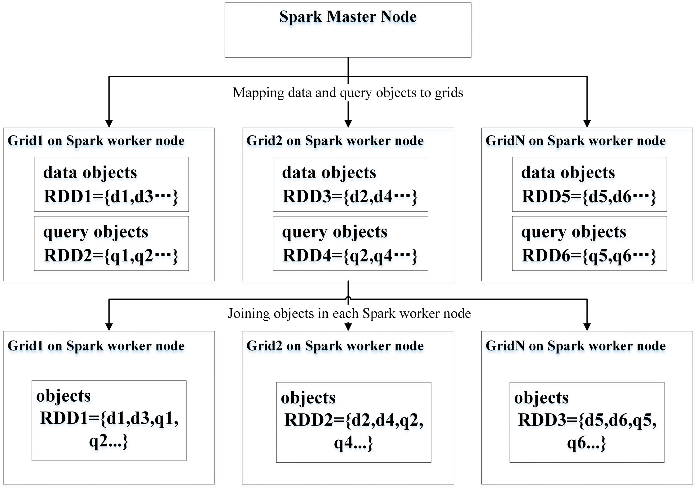
2. Parallel SQPAs Using Spark CM

Let D and Q be a data object collection and a query object collection respectively. Spatial range query (SRQ) represents searching data objects of D related to query objects of Q within a certain distance. The Nearest neighbor query (NNQ) searches the closest data objects to a given query object. The query ‘find the nearest hotels close to a given space’ is an example of NNQ, where the hotels are the data objects and the space is the query object. Spatial join query (SJQ) combines pairs of objects from the two datasets based on their spatial relationships [23]. Before identifying the parameters impacting the efficiency of Spark-based PSQPAs, we briefly introduce the implementation and execution of them.

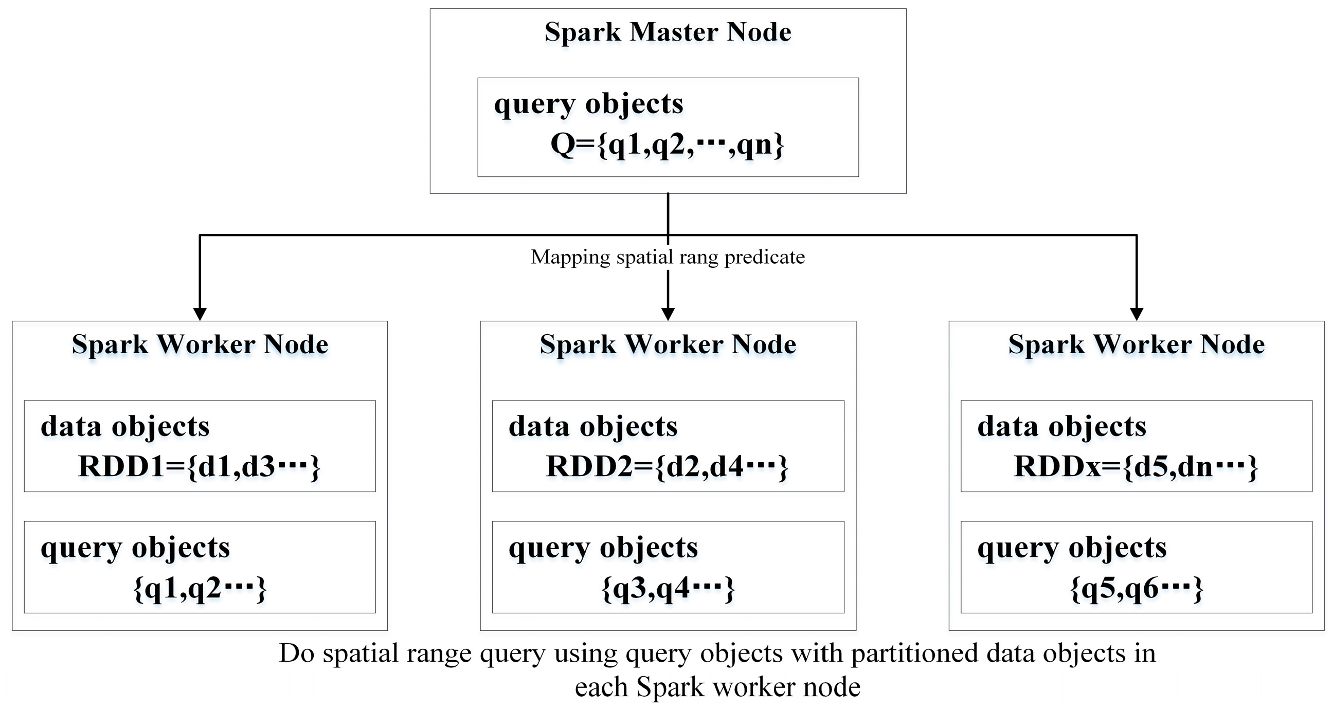
2.1. PSQPAs Using Spark CM

Figure 1 shows the execution of a Spark-based SRQ algorithm (SSRQA). First, spatial data objects are partitioned and stored in distributed nodes. Then, the query objects are broadcast to the nodes where the partitions reside. In these nodes, each query object is used to match the data objects by performing a spatial range predicate computation. We employ GeoSpark for processing large scale spatial data in this work, which is a software package that provides basic geometrical operations. BitTorrent-enabled broadcasting is the main approach for the Spark master to share the immutable objects with Spark workers [10]. Sharing data, the volume of which does not exceed the Java Virtual Machine (JVM) heap size of the Spark master instances, is efficient. Implementation of a simple SSRQA includes only one mapping transformation.
A Spark-based NNQ algorithm (SNNQA) executes as follows. If we suppose that the query objects are small and that the data objects are huge, the query objects can be broadcast to the computing nodes where the partitioned data objects reside. In these nodes, Spark workers execute spatial predicate computations using local spatial data objects. It is assumed that the query objects are too large to be shared, whereas the data objects are relative small. We can then spatially partition the data objects into grids and, if necessary, build an index for them [24]. The grids can then be broadcasted to the computing nodes where the query objects reside. If both the data objects and the query objects are too large to be shared, it is still possible to divide the query objects into chunks and submit the same algorithms with the different chunks as their input. Implementation of a simple SNNQA includes only one mapping transformation. Since the execution flow of a SNNQA is fairly similar to that of a SSRQA, we omit the schematic diagram here in order to save space.
Figure 2 shows a Spark-based SJQ algorithm (SSJQA) that executes as follows. After loading datasets in computing nodes, a Spark engine will partition them into grids according to their approximate spatial location, such as the minimum bounding rectilinear rectangle (MBR). Next, the Spark engine joins the datasets according to their grid IDs [25]. For those spatial objects that have the same grid ID, the spatial overlap that predicates computation is evaluated in the same computing nodes. If two types of objects overlap, they are kept in the final results. Finally, the results are grouped by rectangles with the duplicate objects removed. The implementation of a SSJQA may include several joins, mapping, and filtering transformations.

2.2. Identifying Factors Impacting the Efficiency of Spark-Based PSQPAs

Since the practical method to efficiently query against big spatial data is to employ the divide and conquer strategy [9,26], most MapReduce-based PSQPAs use certain types of space filling curves, such as Hilbert space-filling curve, to map MBRs to grids based on the spatial correlation for optimizing efficiency [27,28]. We simply treat the number of grids p as one of the internal parameters of Spark-based PSQPAs. We focus on SNNQAs exclusively. Since a SSRQA can be seen as a simple case of SNNQAs, the spatial range predicates of the SSRQAs that can be wrapped into a single mapping transformation; that of SNNQAs. SSJQAs are more complex than SNNQAs. The basic units composing this complexity are multiway joins. Although joins are unavoidable and time-consuming, the projection operation mapping spatial correlated datasets into the same grids is commonly used in the filter and refinement stages [28]. From the viewpoint of Spark CM, the number of grids determines the number of tasks that should be executed, which can directly impact the efficiency of the PSQPAs. The projection operation only determines the cost of networking communication. Since building cost models for networking communication is complex, we identify the number of grids as the internal parameters of PSQPAs. Our purpose is to evaluate the relationship between the number of grids and the execution time of the PSQPAs, which may be useful for self-adaptive systems. In this paper, we exclusively use a Spark standalone model because it is easy to configure a Spark cluster without using other frameworks in a cloud computing environment. Moreover, the standalone model demonstrates good reliability, as demonstrated in our earlier work. The parameters of the Spark standalone model include; driver-core, driver-memory, executor-memory, total-executor-cores, and executor-cores. The first two parameters are application-related and defined by users to set the resource requirement for the Spark master instances. The last three parameters are used to set the resource requirement for each of the Spark worker instances. Since the value of the total-executor-cores is an expectation of users who handle large amounts of spatial data, it is considered another impactor. Further, Spark workers running on containers compete with each other for available resources. Therefore, we do not consider the executor-memory and executor-cores as parameters. The other possible parameter of SNNQAs would be the k parameter, which specifies the desired number of the nearest neighbor’s query objects.

3. Horizontal Auto-Scaling Containers for Elastic Spatial Query Processing

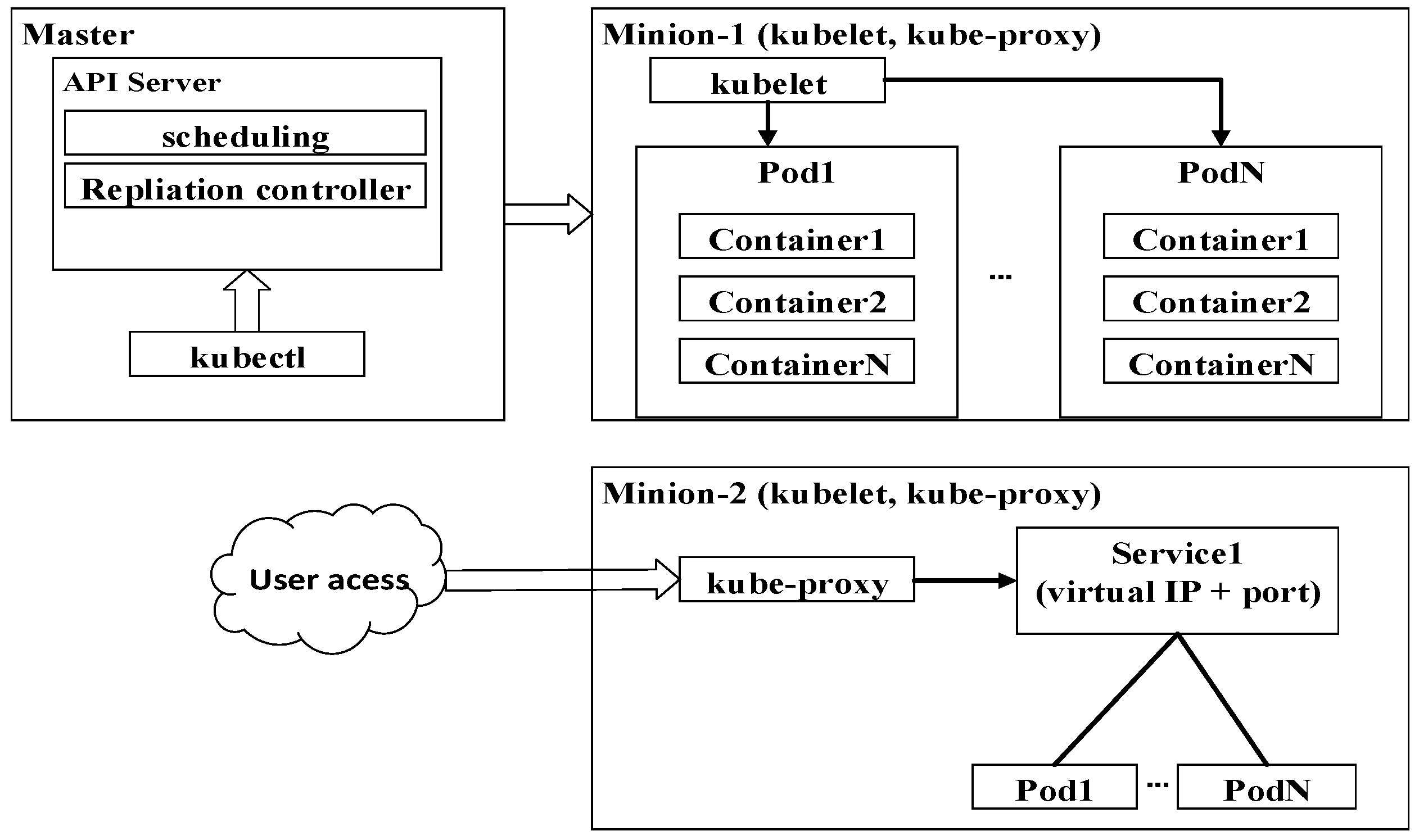
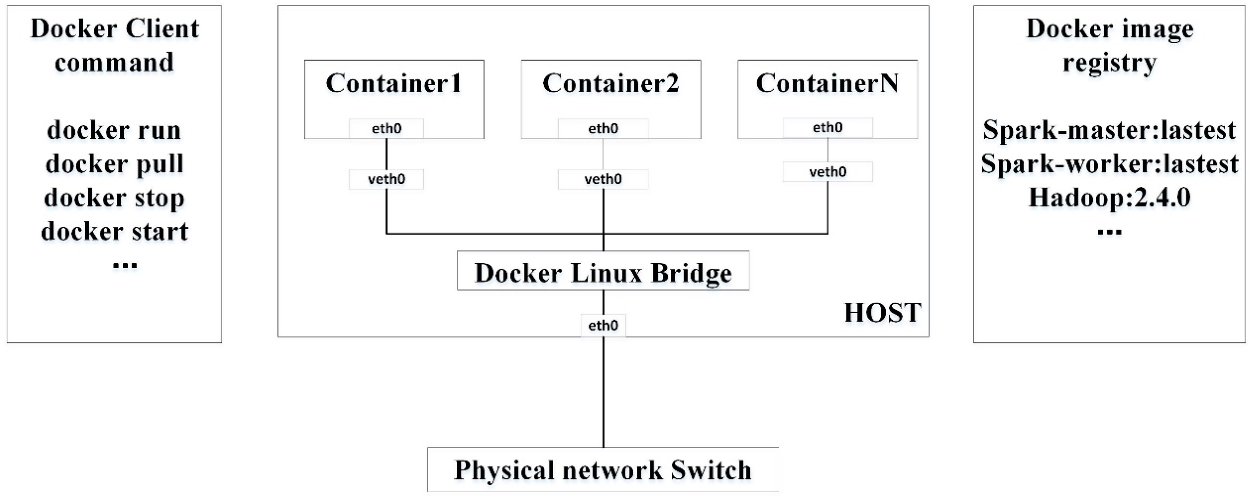
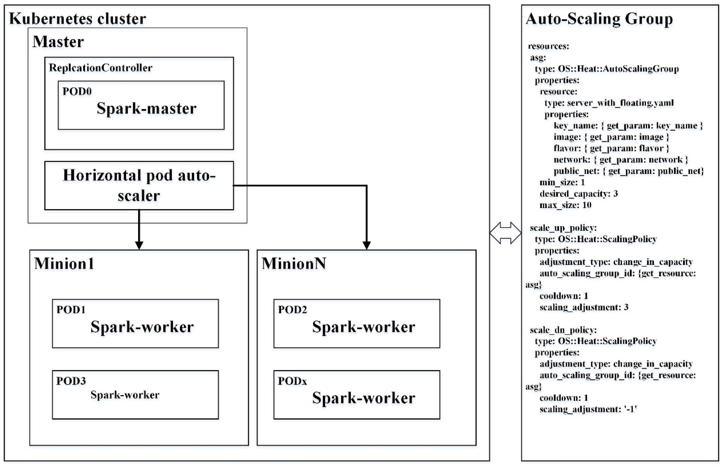
3.1. Docker with Kubernetes Orchestration for Clustering Containers

Our testing system is based on Docker, which is an open source project for automating the deployment of containerized applications in a Linux environment [29]. Docker is a framework that manages the lifecycle of application containers. An application and its dependencies are encompassed into an image. A Docker image can be built from a basic image and other existing images. The basic image is a minimum operating system such as a community enterprise operating system (CentOS), Rancheros, or CoreOS. Applications and a basic image are combined into a single layer-wised image. Layer-by-layer storage facilitates sharing and updating the application components at minimum cost. From Docker’s point of view, a container is the basic management unit in which an application runs. Docker containers share the basic operating system with other containers rather than use another copy. Figure 3 shows how Docker clients would instruct a Docker host to launch containers for running applications with specified images. The Docker image registry is the dedicated gallery for storing the images. We use a private image registry to store Spark-master and Spark-worker images in our tests.
The Docker facilitates application executions in a single host. To fabricate computing clusters using containers, higher level tools such as Docker Swarm and Kubernetes are necessary [30,31]. Docker Swarm is a Docker-native container orchestration system for cluster computing. Since it’s imple and flexible in deployment, it has been widely-used in OpenStack clouds for data analysis [32]. However, containers on different hosts cannot interact with each other without using the current unstable Docker overlay network. Moreover, at the time of this writing, many advanced functionalities such as self-healing and auto-scaling are not supported by Docker Swarm. Kubernetes is another open source project. It was released in June 2014 and originates from the requirement for managing billions of containers in the infrastructure. Kubernetes, which is more complex than Docker Swarm, has been used by Google for decades. The complexities cultivate numerous benefits for containerized applications such as high availability, self-healing, and auto-scaling containers with fine-grained cluster monitoring. Figure 4 shows how Kubernetes adapts master-slave architecture to manage containers in minions. Kubelet and Kube-proxy running on minion, are components for disseminating changing workloads to pods and routing services-oriented access to pods, respectively. Here each pod is a logical group of containers that run on the same application. The Application Programming Interface (API) server is the main services gallery and an access point for Kubectl (a command line interface for running commands against Kubernetes clusters) to query and define cluster workloads. The Kube-scheduler and Kube-controller-manager work with the API server for scheduling workloads in the form of pods and ensuing specified pods replicate running in minions, respectively. For reasons of simplicity, they are not shown in Figure 4.

3.2. Horizontal Auto-Scaling Containers for Elastic Spatial Query Processing

To explore elastic spatial query processing in a cloud computing environment, we assume that there are C cores, I maximum instances, and M gigabytes of memory leased for a tenant. Figure 5 shows the computing resources, which are used as follows. The left part consists of a stable cluster, in which the Kubernetes Master manages containers on a fixed number of minion nodes. A horizontal pod auto-scaler (HPA) is a plugin for Kubernetes that automatically increases and/or decreases the number of pods across the minions. To build a robust Spark cluster on top of Kubernetes, users can request Kubernetes to create a replication controller to ensure one, and only one, Pod that runs the Spark-master image. Kubernetes allows users to explicitly define resource quotas for pods. Therefore, a pod that has sufficient memory, and cores would be exclusively used by the Spark-master instance. Then, the HPA would create an auto-scaling group of containers for Spark-worker instances based on some auto-scaling strategies. Finally, Spark-workers connect to the Spark-master instances by using a Kubernetes service for fabricating an elastic Spark cluster. Kubernetes services are logical groups of pods. They are used for routing the incoming traffic to background pods. Three parameters are mainly used to define the auto-scaling strategies. The minReplicas and maxReplicas parameters declare the minimum and maximum number of pods allowed, respectively. Kubernetes calculates the arithmetic mean of the pods’ CPU utilization with the target value, as defined by the target percentage parameter, and if necessary adjusts the number of pods allowed. The right part includes an auto-scaling group, in which virtual machines (VMs) scale in and scale out according to the policies defined in the Heat templates. The minimum and maximum size properties of an auto-scaling group are used to define the threshold of instances allowed for cloud users. To horizontally scale Docker containers in an auto-scaling group, the preliminary requirement is that the VMs can automatically join the Kubernetes cluster. Fortunately, the cloud-config files of OpenStack can be used in this context [33]. The loading of the kube-proxy and kubelet services on the minion nodes can be done automatically on the boot of the VMs.
This proposed empirical strategy divides the computing resources into two parts and provides a way to distribute the containers over all the nodes. By separating the Spark-master and Spark-workers into containers and leveraging the HPA to distribute the workload, we can build self-healing Spark clusters to process huge volumes of spatial datasets. The experiments and results are presented in Section 4.

4. Experiments and Results

4.1. Spatial Datasets for A Spatial Query Processing Case

In this paper, we introduce the concept of spatial datasets to better understand patterns of human mobility in urban areas. In order to perform this analysis, which is fundamental for city planners, trajectory data are collected from inexpensive GPS-equipped devices, such as taxicabs. Taxi trip data is widely-used for mining traffic flow patterns, as described in [34,35]. For example, the NYC Open Data Plan has built a portal for publishing its digital public data for city-wide aggregation, as required by local law. In addition, the New York City Taxi and Limousine Commission has published, since 2009, taxi trip data sets to the portal. In 2015, a total of 11,534,883 rows of green taxi trip data were recorded. The records include field capturing, pick-up and drop-off dates, times, locations, distances, payment types, and driver-reported passenger counts. Since the pick-up and drop-off locations are just pairs of geographical coordinates, additional spatial data sets that include land use type (LUT) are required. We collected a data set named NYC MapPluto Tax Lot from the NYC Department of City Planning. The fields in the data set include LandUse, XCoord, and YCoord, which describe the land use categories such as Family Building, Commercial and Office Buildings, Industrial and Manufacturing, and the approximate location of the lots. The Tax Lot dataset contains 834,158 records. A taxi customer’s pick-up location near a Family Building and drop-off location near a Commercial and Office Building at rush hour, indicates that the person’s taxi request may be work related. We explore the data sets with the previously mentioned SNNQAs. Readers can find the datasets by using the following links: https://data.cityofnewyork.us/Transportation/2015-Green-Taxi-Trip-Data/n4kn-dy2y and http://www1.nyc.gov/site/planning/data-maps/open-data.page (last access date: 2017/2/8)

4.2. Cloud Computing Environemt

There are six machines used for setting-up our OpenStack cloud. The Liberty version of OpenStack, released to public in October 2015, was choosen. As shown in Table 1, the controller node is a commodity PC equipped with 1 processor, 4 cores, 4 GB memory, and 500 GB disks, on which the Keystone identity service, Telemetry service, Neutron networking service, and Glance service run. The Neutron Linux bridge agents running on computing nodes are connected with each other to fabricate networking for virtual instances. We use four Dell PowerEdge M610 servers to build the computing nodes clusters, with one of them having two physical CPUs, 24 cores, 92 GB of main memory, and a 160 GB disk, and three of them having two physical CPUs, 24 cores, 48 GB of main memory, and a 500 GB disk. The block storage node is a HP Z220 workstation configured with two physical CPUs, 8 cores, 32 GB of main memory, and 3 TB disks. The Cinder services running on the HP workstation is using Network File System (NFS) to provide virtual instance with storage. To simulate complex network infrastructure, we let the computing nodes traverse two different subnets. 1000 Mbps networking devices are used to bridge the two subnets. All nodes in the cloud computing environment adapt a Ubuntu 14.04.4 LTS 64 bits operating system. All required packages that support the OpenStack cloud are installed with their native package. More specifically, RabbitMQ 3.5.4 is used for coordinating operations and status information among services. MariaDB 5.5.52 is used for services to store data. The libvirt KVM and Linux Bridge are used to provide platform virtualization and networking for virtual instances. We exclusively use the vxlan mechanism to provide networking with virtual instances. For some convenience, we abbreviate the auto-scaling VM instances and the auto-scaling Docker containers as ASVI and ASVC, respectively.

4.3. Result

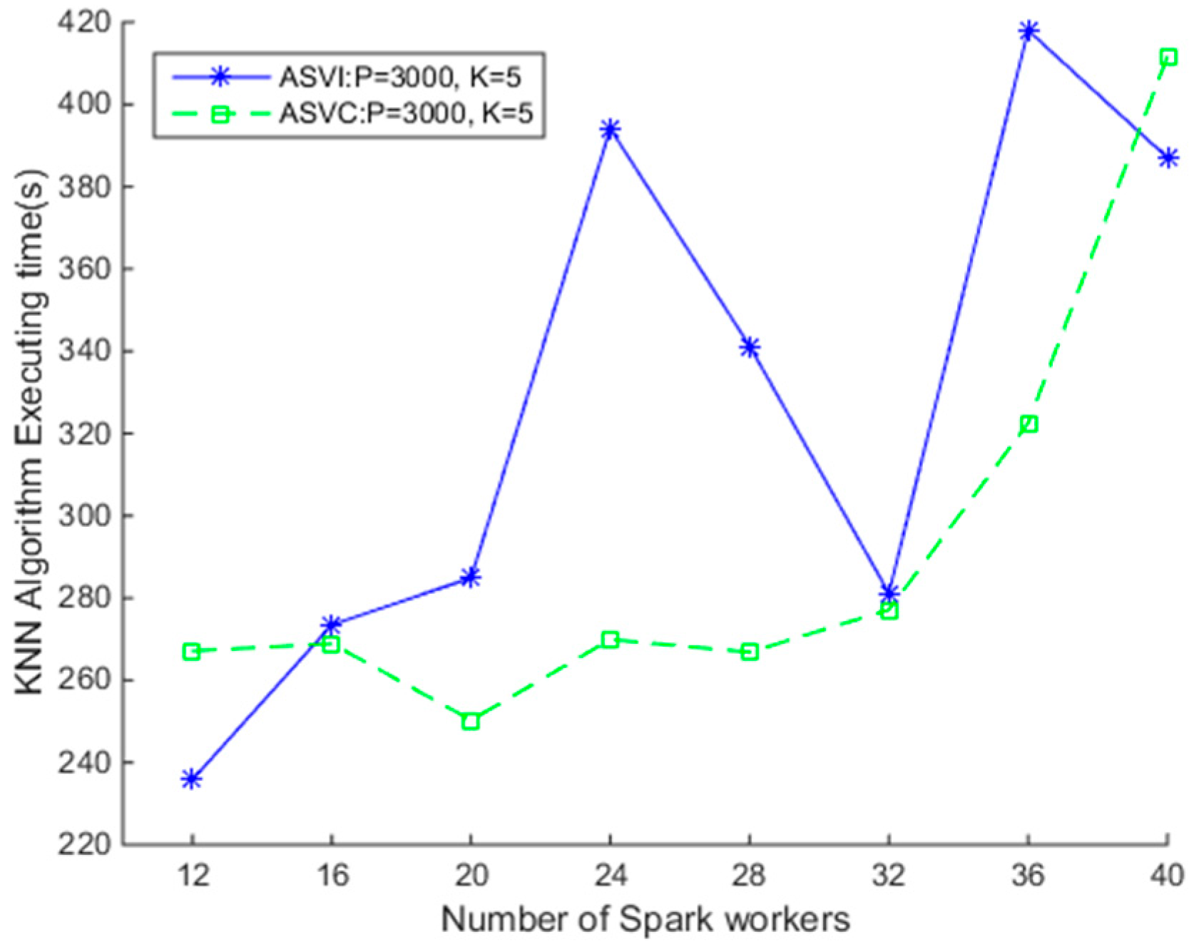
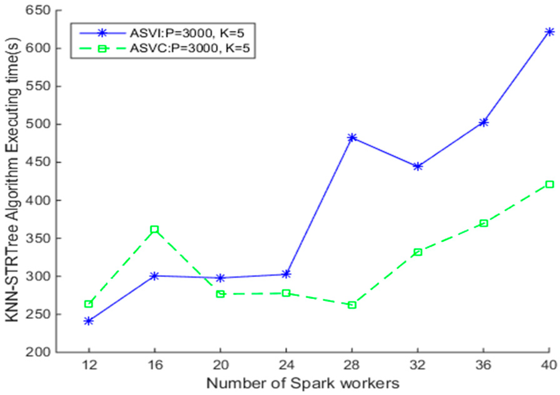
4.3.1. Comparison of SNNQAs using ASVI and ASVC

To test the efficiency of SQP using ASVI and ASVC, we construct two clusters using two OpenStack Heat templates. As shown in Table 2, the only difference between the clusters is the image and software used. The two clusters can be comparable in this context, since the deployment of instances on which computing nodes can be exactly specified by using an OS::Nova::Server availability zone property in Heat templates. In the Ubuntu cluster, the node having 4VCPUs and 8 GB of memory hosts the Spark master instance, while the other four instances host the Spark worker instances. In the CoreOS cluster, the nodes holding each type of Spark component are determined at runtime. More specifically, the softwares and their versions are listed in Table 3.
Assuming the clusters’ launching time is negligible, we first test the efficiency of the SNNQAs under the two clusters. Since it is necessary to specify the Ubuntu image in advance, the number of Spark workers running on each virtual instance is the same when using the ASVI. As shown in Figure 6, the efficiency of SNNQAs using the two auto-scaling strategies on the OpenStack cloud is very different. When p = 3000 and k = 5, there are 3000 grids on which to store spatial data objects, and each query object queries the five nearest spatial data objects in the grids. The average execution time is recorded when each SNNQA submission is executed 10 times with the total-executor-cores parameter set to six. We observe that increasing the number of Spark workers does not guarantee better efficiency of the algorithms. For example, when there are 12 Spark workers, the average execution time of the SNNQA using the ASVI strategy is 235.84 s. Doubling the number of Spark workers to 24 raises the average execution time of the SNNQA using the ASVI strategy (SNNQA-ASVI) to nearly 400 s, and when the number of Spark workers is increased to 32, the average execution time of the SNNQA-ASVI falls to 281.18 s. Then, when we increase the number of Spark workers to 36, the average time cost of the SNNQA-ASVI rises to 420 s. The high SNNQA-ASVI efficiency variability is possibly due to two factors; (1) the performance disturbance of the virtual instances and (2) the uncertainty of the number of Spark workers introduces SNNQA variations using the ASVI. We notice that Spark workers are quite often lost in the tests. Data-intensive computational tasks executed on each Spark worker require too many memory resources, which may disrupt the connection between the Spark workers and the Spark master instance. Further, there are no self-healing mechanisms for Spark workers in this context. When given fewer than 28 Docker containers to the algorithm, the execution time is always less than 270 s. As the results in Figure 6 show, when given 24 Docker containers, the average execution time is 269.91 s. When the number of Docker containers is limited to 20, the average execution time falls to 250.31 s. The time cost of the SNNQAs, using the two strategies, grows rapidly when the number of Spark workers is more than 32. These results indicate that the SNNQAs using the ASVC could be robust if the Docker container number is smaller than 32.
To investigate the effectiveness of the index to the SNNQAs, we conduct the second experiment as follows. When using the ASVI and 20 Spark workers, the Spark-based KNN algorithms using the Sort-Tile-Recursive tree (STRtree) index (SKNN-STRtree) completes in about 297.92 s, as shown in Figure 7. The Spark-based KNN algorithms without the STRtree index complete in about 284.89 s, as shown in Figure 6. These results indicate that using the index does not reduce the execution time of the SNNQAs using the ASVI strategies. The reason may be because the number of data objects in the grids is not large; therefore indexing in this context may not be necessary. The grid number determines the average number of objects that are processed by each Spark worker. When the grid number is small, the number of objects is large. Each Spark worker consumes more memory and increases the amount of time spent executing the spatial predicate calculation. When the grid number is large, the number of objects is small. When using the ASVC, the Spark-based K Nearest Neighbor (KNN) algorithms using the STRtree index complete in less than 300 s if working with 20 to 28 containers. These results indicate that the SNNQAs with the STRtree index using the ASVC could be robust if the container number is smaller than 28, and when giving more than 28 containers to the Spark workers, the costs of the SKNN-STRtree obviously increase. These results indicate that the CoreOS cluster may be too small for Kubernetes to auto-scale many containers. We also notice that the efficiency of the SKNN-STRtree varies when using the ASVI strategy. These similar results indicate that, regardless of whether or not indexing is used, the efficiency of the SNNQAs using the ASVI strategy is highly variable in clouds. The number of Spark worker daemons running on virtual instances varies. The Spark daemons residing on each virtual instance are prone to be out of service for many reasons. Data-intensive tasks consume lots of the memory of a Spark worker instance, which may lead to an ‘out of memory’ error. Additionally, networking in the cloud is typically unstable, and the networking between the Spark workers and the Spark master can sometimes be broken. We observe that the Spark worker daemons frequently fail during the tests. Therefore, we focus our remaining research, in this paper, exclusively on the ASVC strategies.

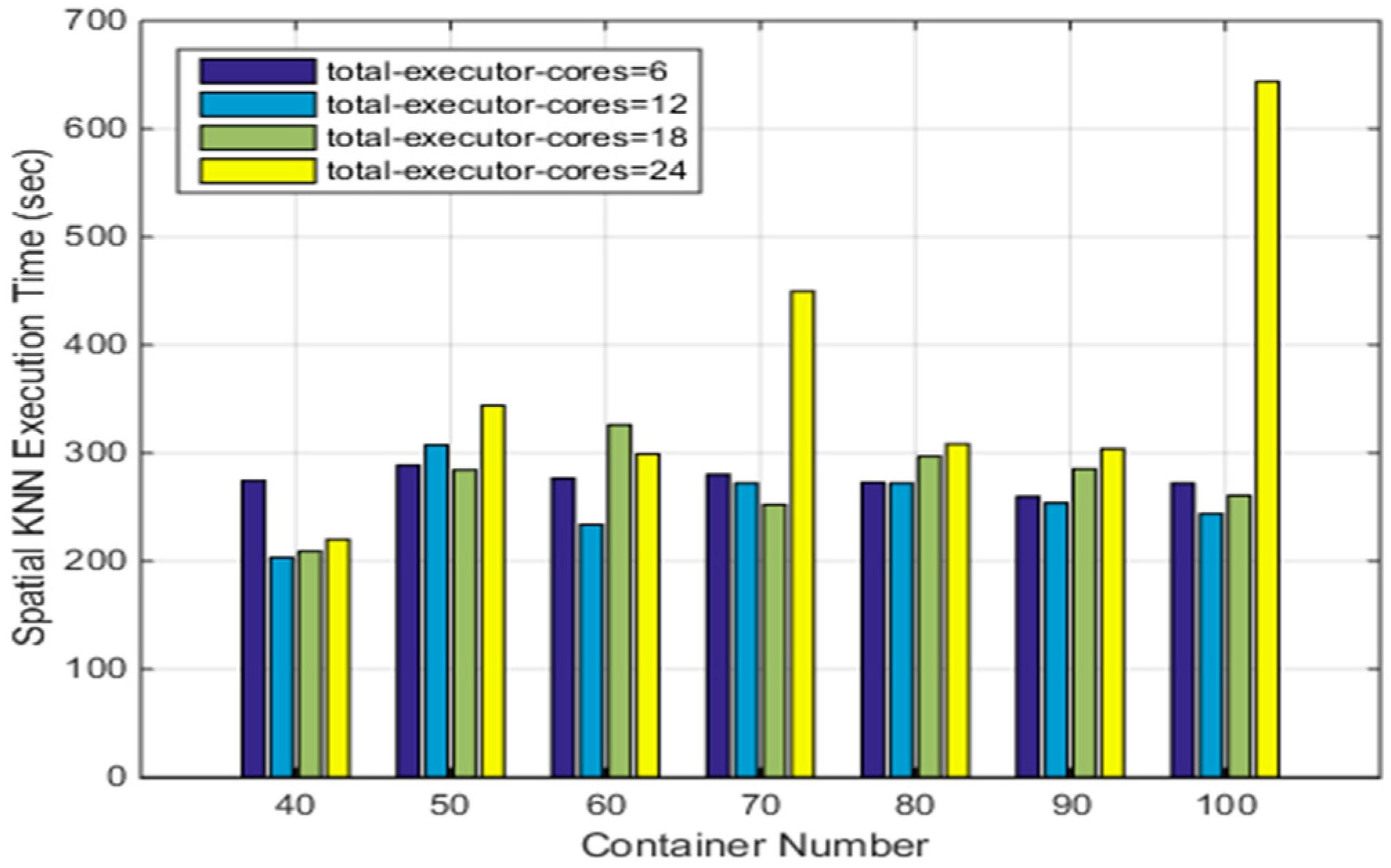
4.3.2. SNNQAs Using ASVC

To understand how the parameter p impacts the efficiency of the SNNQAs, we conduct the third experiment as follows. Each submission of the SNNQA using the ASVC is executed 10 times with the total-executor-cores parameter set to six, and the average execution time is recorded. As shown in Figure 8, when there are fewer than 32 Docker containers relative to Spark workers, the SNNQAs complete in less than 300 s. When setting p = 3000, k = 5, and using 20 Docker containers, the average minimum execution time of the SNNQAs is about 250 s. When setting p = 2500, k = 5, and using 20 Docker containers, the average minimum execution time of the SNNQAs is about 270 s. When setting p = 2000, k = 5, and using 20 Docker containers, the average minimum execution time of the SNNQAs is about 271 s. We found that reducing the value of parameter p would increase the execution time of SNNQAs in this context. For example, when setting p = 1500, k = 5, and using 20 Docker containers, the average minimum execution time of the SNNQAs is about 330 s. When setting p = 1000, k = 5, and using 20 Docker containers, the average minimum execution time of the SNNQAs is about 437 s. The results testified that Spark is more suitable for handling small parallel tasks. As discussed earlier, the parameter p controls the number of parallel tasks at each stage of the Spark transformation chains. When the parameter p is small, the number of spatial objects processed by each Spark executor would be large, and the latency of the algorithms would thereafter increase. We do not explicitly state which configuration is best in this paper, but the curves of the average execution time of the SNNQAs using the ASVC exhibits great consistence when the Docker container number is fewer than 32. Our testing reveals that Spark workers running on the same host communicate with each other at low cost; therefore the performance of the SNNQAs is reliable. We observe that when more than 32 Docker containers are given to Spark workers, the execution cost of the SNNQAs increases, mainly because Kubernetes cannot sustain the required number of containers in the small CoreOS clusters.
k is an important parameter for the SNNQAs and, according to our tests, demonstrates a similar pattern to our parameter p observation. In the interest of saving space, the results are not depicted in this paper. We prefer to know the efficiency of the SNNQAs using the ASVC in large clusters. Therefore, we conduct a fourth experiment as follows. A CoreOS cluster with 19 virtual instances is built in which one instance has four VCPUs and 8 GB of RAM, and other instances each have two VCPUs and 4 GB of RAM. The average execution time is recorded for each of the 10 submissions. As shown in Table 4, when setting the total-executor-cores parameter to six, the SNNQAs with different parameters complete in less than 300 s. The average execution time of the SNNQAs is from 259.53 s to 288.50 s. When providing 90 Docker containers with Spark workers, the average execution time of the SNNQAs is about 259.53 s. The results have verified our earlier discussion. In a small Kubernetes cluster, a large number of Docker containers may pose higher completion to the underlying OS, which is the primary reason that the efficiency of the SNNQAs declines. Although Kubernetes enables auto-scaling hundreds and even thousands of containers in a few seconds, we suggest not using a large number of Docker containers in small clusters in order to avoid overloading.
Since the CoreOS cluster has a total of 40 cores, the value of the parameter ‘total-executor-cores’ can be larger than six in the above tests. To understand the impact of the Docker container number on the efficiency of the SNNQAs using more cores, we conduct our fifth experiment as follows. Each submission of an SNNQA using ASVI is executed 10 times with p = 3000 and k = 5, and the average execution time is recorded. As shown in Figure 9, when the value of the ‘total-executor-cores’ is from 6 to 18, the average execution time is about 300 s. Even when the Docker container number is set to 100, the time cost never exceeds 300 s. However, the performance varies when there are 24 total-executor-cores. For example, when giving 50 Docker containers to Spark workers, the average execution time is 343.92 s. When increasing the number of Docker containers given to the Spark workers to 70, the average execution time rises to more than 400 s. Increasing this number of Docker containers further, to 90, reduces the average execution time down to approximately 300 s. These results indicate that the container number and total executor cores used by Spark workers are the determining factors for the performance of the SNNQAs. When giving 40 Docker containers for Spark workers and setting the total-executor-cores to 12, the average execution time of the SNNQAs is 203.33 s. Using the same number of Docker containers for Spark workers but increasing the number of total-executor-cores to 18 increases the SNNQAs’ average execution time to 208.93 s. These results indicate that if we choose a relatively small number of Docker containers with moderate total executor cores for Spark workers, the SNNQAs’ performance reliability and efficiency increase. It is important to note that the time cost of the SNNQAs is nearly 300 s when giving six, 12, and 18 cores to Spark workers. We observe that the overall performance of the SNNQAs using 12 cores is more robust than that using six and 18 cores. The total-executor-cores parameter is an upper threshold that represents the maximum number of cores that Spark worker containers can consume. As more cores are given to Spark workers, the number of chances for each Spark worker to execute tasks increases, but the larger value of the parameter also introduces more scheduling tasks for the Kubernetes scheduler. This situation is clear when we use a larger number of Docker containers since Kubernetes would take more time to assure that the specified number of Docker containers is ready. The larger the number of total executor cores used by Spark workers, the greater the amount of competition that occurs between containers that run Spark worker daemons. Kubernetes takes more time to reschedule crashed Spark workers, which in this situation causes the Spark master instance to reschedule failed tasks. The execution of the SNNQAs was about 625 s when giving 30 cores to Spark workers and setting the container number to 50, and execution of the SNNQAs always failed when giving 30 cores to Spark workers with more than 60 containers.

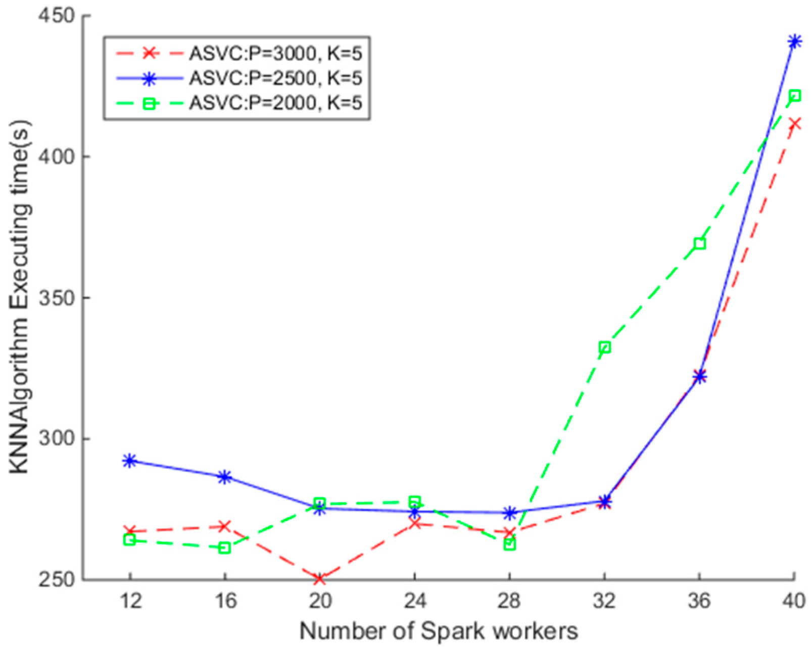
4.3.3. SNNQAs Using Different ASVC Strategies

To investigate the efficiency of the SNNQAs using different auto-scaling strategies, we conduct the sixth experiment as follows. A Heapster plugin is used to collect CPU workload metrics from kubelet daemons. Each submission of the algorithm is executed 10 times and the average execution time is recorded. As shown in Table 5, when the MinReplicas, MaxReplica, and TargetPercentage are set to 1%, 40%, and 50% respectively, the average execution time of the SNNQAs is 303.49 s. When the values of the MinReplicas, MaxReplica, and TargetPercentage parameters are 10%, 40%, and 50% respectively, the average execution time of the SNNQAs is 247.68 s. These results indicate that the minimum number of replicas of Spark workers guaranteed by Kubernetes has a certain impact on the efficiency of the SNNQAs, but the impact is not clear, as observed in our testing. For example, when we set the values of the MinReplicas, MaxReplica, and TargetPercentage to 1%, 40%, and 80% respectively, the average execution time of the SNNQAs is 272.56 s. When the values of the MinReplicas, MaxReplica, and TargetPercentage parameters are 10%, 40%, and 80% respectively, the average execution time is 249.89 s. We observe that the number of containers never grows to 40 when we set the value of the MinReplicas parameter to 10%, 20%, and 30% because of two factors. The first reason is that Kubernetes master fails to calculate the averaged CPU workload in the very short period of each submission. The second reason is that the Heapster plugin may fail to collect the metrics for the containers. Our goal, in the near future, is to find alternatives that provide real time monitoring for Kubernetes. Although there are still some flaws in the auto-scaling strategies, we observe that when setting the value of the MinReplicas to 1%, an HPA works well in all the tests.

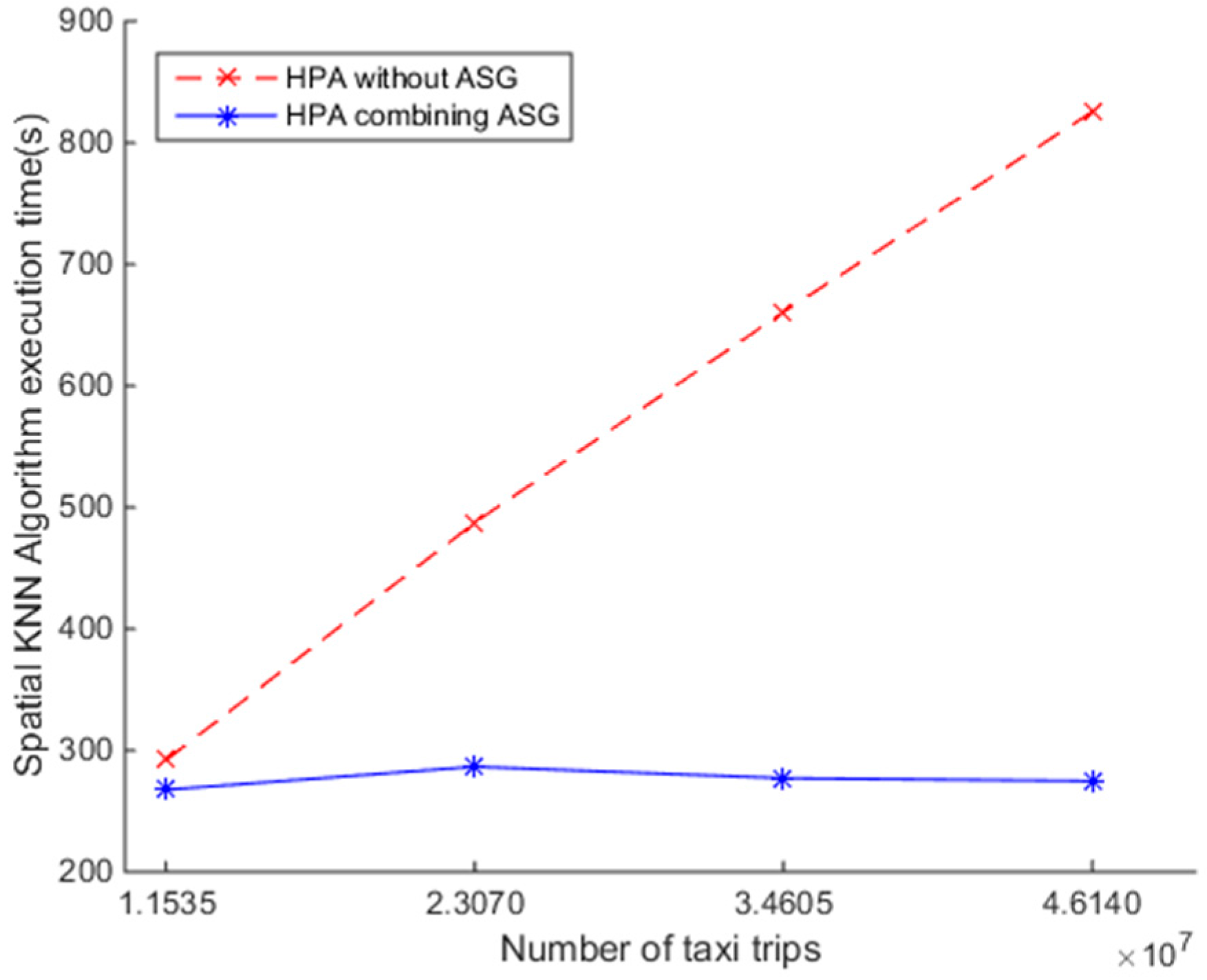
4.3.4. SNNQAs Using ASVC in an Auto-Scaling Group

To investigate the efficiency of the SNNQAs using an HPA combined with an auto-scaling group, we conduct the seventh experiment as follows. First, a Heat template is used to depict the minimum, the desired, and the maximum number of CoreOS instances, which should be 5, 5, and 10, respectively. Each CoreOS instance has two VCPUs and 4 GB of RAM. Next, we force the auto-scaling group to scale out when the CPU utilization rate is above 80% and lasts about 1 min. Second, a Kubernetes template is used to depict the values of the minimum and maximum replicas of Spark workers, which should be 1 and 200, respectively. The TargetPercentage parameter is set to 80%. Finally, the SNNQAs are submitted to the auto-scaling group using the parameters: total-executor-cores = 18, p = 3000, and k = 5. Each submission of the SNNQAs is executed five times and the average execution time is recorded. As shown in Figure 10, increasing the number of query objects monotonically increases the execution time of the SNNQAs using the HPA exhibits when the auto-scaling group is not used. Finding the five nearest neighbors from 834,158 spatial data objects for each of the 34,604,649 query objects took approximately 660.64 s, while the execution time that uses the HPA combined with the auto-scaling group results in great performance. All of the runs complete in less than 300 s. The results show that the HPA combined with the auto-scaling group is beneficial for reliable spatial big data analysis. It is suggested that future research be directed toward automatically configuring these parameters.

5. Discussion

Elasticity is one of the main characteristics of cloud computing, which means that computing resources can be increased or decreased in a dynamic and on demand way according to the current workload of applications [17]. Current solutions direct use of the auto-scaling groups to spawn VMs on which a dedicated VM is used to run Spark master daemons and other VMs are used to run Spark worker daemons. Since the performance variability of VMs running Spark master daemons can impact the scheduling tasks of the Spark engine, it may be less likely to build useful regression models for estimating the execution time of Spark-based PSQPAs. Moreover, the Spark master and worker daemons running on VMs can be out of work without using an additional recovery mechanism. Additionally, the capacity of the dedicated VM would be over-provisioned or under-provisioned let alone the computing resource ineffectively used. As shown in Figure 6, when using the ASVI strategies, the efficiency of the SNNQAs is highly variable. Since each Spark worker daemon consumes a fixed number of memory resources on the Ubuntu VMs, we cannot specify a large value to the number of Spark workers that run on the same VM. During our testing, we observed that Spark worker daemons are frequently lost. This may be correlated with the Transmission Control Protocol (TCP)-oriented Netty protocol used for receiving the commands from the Spark master and transmitting data between Spark workers. If the connection is lost, then Spark workers would be out of services. In addition, the limited memory space of Spark executors can’t satisfy the computation requirement when handling too much data or too many query objects. The relationship between the number of Spark worker daemons running on VMs and the execution time of the SNNQAs is indefinite. To satisfy time-constrained data analysis, the uncertainty should be removed. The performance variability of the VMs and the lack of a self-healing mechanism for Spark workers running on VMs preclude us from using an ASVI strategy, while the overall performance of SNNQAs using ASVC is more stable than that using ASVC strategies. The time costs of SNNQAs could complete in less than 280 s if we provide less than 28 Docker containers in this context. We notice that the time cost grows rapidly when using more than 32 containers for Spark workers and an ASVC strategy. The reason may be highly correlated with the kernel burden for switching processes, and the completion between Kubernetes pods would be high. Since Kubernetes adapts an implicit optimization policy that always tries to achieve the specified status according to the current available resource, the scheduler would take more time to reassign the failed containers to proper nodes. Compared with VMs, Linux containers demonstrate equal or better performance under various workloads [22].As shown in Figure 8, SNNQAs using ASVI strategies complete in less than 300 s when fewer than 32 containers for Spark workers are used. Other than self-healing containers, Kubernetes facilitates auto-scaling containers to all available computing nodes through the use of an HPA. We also explore the relationship between the execution time of SNNQAs and the number of containers in large clusters. Figure 9 shows that a small number of containers with a moderate number of total executor cores used by Spark, results in robust executions of the SNNQAs. The relationship is definite when the total executor cores do not exceed the number of virtual cores of all available VMs. Lastly, we check the feasibility of an HPA combined with an auto-scaling group for the elastic provision of containers in a scale-out manner. The results, as shown in Figure 10, indicate that an HPA combined with an auto-scaling group is useful for predicting an SQP in a cloud computing environment. Although tremendous efficiency can be obtained when an HPA is used, we observe that the Heapster plugin sometimes fails to collect CPU metrics, which may impact auto-scaling container strategies. Another shortage is that Spark components running in Docker containers have no simple way to share data and software packages. We use the volume NFS image for sharing data among Kubernetes Pods, which may impact the total execution time of SNNQAs. This is an area future research.

6. Conclusions

In this paper, we proposed an elastic spatial query processing approach in an OpenStack cloud computing environment by using Kubernetes-managed Docker containers for auto-scaling an Apache Spark computing engine. By leveraging the self-healing and auto-scaling mechanism of Kubernetes and utilizing the in-memory computing paradigm of Spark, we can build an elastic cluster computing environment for spatial query processing in a cloud computing environment. To satisfy time-constrained data analysis, we introduces the implementation of Spark-based spatial query processing algorithms (SQPAs) in this paper, and then we identified three factors that would impact the execution time of SQPAs. The first factor is the internal parameters of the SQPAs, which includes the number of grids p that are used for grouping spatial correlation datasets. Since the Spark engine is suitable for tackling tremendous but relatively small tasks, we suggested using a large value of the parameter p and considering the volume of spatial datasets and the underlying computing resource. The second factor is the parameters of the Spark computing model such as total-executor-cores. For example, an inappropriate number of total executor cores used by the Spark engine would bring about intense completion between containers. We suggested using a small number of containers with a moderate number of total executor cores for reliable spatial query processing of big spatial data. The last factor is the parameters used for defining auto-scaling strategies. For example, MinReplicas, MaxReplica, and Targetpercentage parameters would impact the execution time of SQPAs. The experiments and the tests conducted on an OpenStack cloud computing platform indicate a chance for time-constrained SQPAs. Considering the parameters, our future work will investigate how to build cost models for Spark-based spatial query algorithms that use the ASVC strategies and how to automate the settings of these parameters in OpenStack clouds for processing spatial big data in the big data era.

Acknowledgments

We gratefully acknowledge funding support for this research provided by the National High-Resolution Earth Observation System Projects (civil part): Hydrological monitoring system by high spatial resolution remote sensing image (first phase) (08-Y30B07-9001-13/15).

Author Contributions

Wei Huang designed the experiment and procedure, Wen Zhang analyzed the results, and they both wrote the manuscript. The work was supervised by Lingkui Meng, who contributed to all stages of the work. Dongying Zhang made major contributions to the interpretations and modification.

Conflicts of Interest

The authors declare no conflict of interest.

References

  1. Lee, J.G.; Kang, M. Geospatial big data: Challenges and opportunities. Big Data Res. 2015, 2, 74–81. [Google Scholar] [CrossRef]
  2. Yang, C.; Huang, Q.; Li, Z.; Liu, K.; Hu, F. Big data and cloud computing: Innovation opportunities and challenges. Int. J. Digit. Earth 2017, 10, 13–53. [Google Scholar] [CrossRef]
  3. Li, S.; Dragicevic, S.; Castro, F.A.; Sester, M.; Winter, S.; Coltekin, A.; Pettit, C.; Jiang, B.; Haworth, J.; Stein, A. Geospatial big data handling theory and methods: A review and research challenges. ISPRS J. Photogramm. Remote Sens. 2016, 115, 119–133. [Google Scholar] [CrossRef] [Green Version]
  4. Li, Z.; Yang, C.; Liu, K.; Hu, F.; Jin, B. Automatic scaling hadoop in the cloud for efficient process of big geospatial data. ISPRS Int. J. Geo-Inf. 2016, 5, 173. [Google Scholar] [CrossRef]
  5. Yang, C.; Goodchild, M.; Huang, Q.; Nebert, D.; Raskin, R.; Xu, Y.; Bambacus, M.; Fay, D. Spatial cloud computing: How can the geospatial sciences use and help shape cloud computing? Int. J. Digit. Earth 2011, 4, 305–329. [Google Scholar] [CrossRef]
  6. Aji, A.; Wang, F. High performance spatial query processing for large scale scientific data. In Proceedings of the SIGMOD/PODS 2012 PhD Symposium, Scottsdale, AZ, USA, May 2012; ACM: New York, NY, USA, 2012; pp. 9–14. [Google Scholar]
  7. Orenstein, J.A. Spatial query processing in an object-oriented database system. In ACM SIGMOD Record; ACM: New York, NY, USA, 1986; Volume 15, pp. 326–336. [Google Scholar]
  8. You, S.; Zhang, J.; Gruenwald, L. Large-scale spatial join query processing in cloud. In Proceedings of the 2015 31st IEEE International Conference on Data Engineering Workshops (ICDEW), Seoul, Korea, 13–17 April 2015; pp. 34–41.
  9. Zhong, Y.; Han, J.; Zhang, T.; Li, Z.; Fang, J.; Chen, G. Towards parallel spatial query processing for big spatial data. In Proceedings of the 2012 IEEE 26th International Parallel and Distributed Processing Symposium Workshops & PhD Forum (IPDPSW), Shanghai, China, 21–25 May 2012; pp. 2085–2094.
  10. Huang, W.; Meng, L.; Zhang, D.; Zhang, W. In-memory parallel processing of massive remotely sensed data using an apache spark on hadoop yarn model. IEEE J.Sel. Top. Appl. Earth Obs. Remote Sens. 2016, 10, 3–19. [Google Scholar] [CrossRef]
  11. Zaharia, M.; Chowdhury, M.; Das, T.; Dave, A.; Ma, J.; McCauley, M.; Franklin, M.J.; Shenker, S.; Stoica, I. Resilient distributed datasets: A fault-tolerant abstraction for in-memory cluster computing. In Proceedings of the 9th USENIX Conference on Networked Systems Design and Implementation, San Jose, CA, USA, April 2012; USENIX Association: Berkeley, CA, USA, 2012; p. 2. [Google Scholar]
  12. Zaharia, M.; Xin, R.S.; Wendell, P.; Das, T.; Armbrust, M.; Dave, A.; Meng, X.; Rosen, J.; Venkataraman, S.; Franklin, M.J. Apache spark: A unified engine for big data processing. Commun. ACM 2016, 59, 56–65. [Google Scholar] [CrossRef]
  13. Yu, J.; Wu, J.; Sarwat, M. Geospark: A cluster computing framework for processing large-scale spatial data. In Proceedings of the 23rd SIGSPATIAL International Conference on Advances in Geographic Information Systems; ACM: New York, NY, USA, 2015; p. 70. [Google Scholar]
  14. Tang, M.; Yu, Y.; Malluhi, Q.M.; Ouzzani, M.; Aref, W.G. Locationspark: A distributed in-memory data management system for big spatial data. Proc. VLDB Endow. 2016, 9, 1565–1568. [Google Scholar] [CrossRef]
  15. Ray, S.; Simion, B.; Brown, A.D.; Johnson, R. Skew-resistant parallel in-memory spatial join. In Proceedings of the 26th International Conference on Scientific and Statistical Database Management; ACM: New York, NY, USA, 2014; p. 6. [Google Scholar]
  16. Herbst, N.R.; Kounev, S.; Reussner, R. Elasticity in cloud computing: What it is, and what it is not. In Proceedings of the 10th International Conference on Autonomic Computing (ICAC 13), San jose, CA, USA, 26–28 June 2013; pp. 23–27.
  17. Galante, G.; De Bona, L.C.E.; Mury, A.R.; Schulze, B.; da Rosa Righi, R. An analysis of public clouds elasticity in the execution of scientific applications: A survey. J. Grid Comput. 2016, 14, 193–216. [Google Scholar] [CrossRef]
  18. Leitner, P.; Cito, J. Patterns in the chaos—a study of performance variation and predictability in public iaas clouds. ACM Trans. Internet Tech. (TOIT) 2016, 16, 15. [Google Scholar] [CrossRef]
  19. Lorido-Botran, T.; Miguel-Alonso, J.; Lozano, J.A. A review of auto-scaling techniques for elastic applications in cloud environments. J. Grid Comput. 2014, 12, 559–592. [Google Scholar] [CrossRef]
  20. Kang, S.; Lee, K. Auto-scaling of geo-based image processing in an openstack cloud computing environment. Remote Sens. 2016, 8, 662. [Google Scholar] [CrossRef]
  21. Soltesz, S.; Pötzl, H.; Fiuczynski, M.E.; Bavier, A.; Peterson, L. Container-based operating system virtualization: A scalable, high-performance alternative to hypervisors. In ACM SIGOPS Operating Systems Review; ACM: New York, NY, USA, 2007; pp. 275–287. [Google Scholar]
  22. Felter, W.; Ferreira, A.; Rajamony, R.; Rubio, J. An updated performance comparison of virtual machines and linux containers. In Proceedings of the 2015 IEEE International Symposium on Performance Analysis of Systems and Software (ISPASS), Philadelphia, PA, USA, 29–31 March 2015; pp. 171–172.
  23. Brinkhoff, T.; Kriegel, H.-P.; Seeger, B. Efficient Processing of Spatial Joins Using R-trees; ACM: New York, NY, USA, 1993; Volume 22. [Google Scholar]
  24. Akdogan, A.; Demiryurek, U.; Banaei-Kashani, F.; Shahabi, C. Voronoi-based geospatial query processing with mapreduce. In Proceedings of the 2010 IEEE Second International Conference on Cloud Computing Technology and Science (CloudCom), Indianapolis, IN, USA, 30 November–3 December 2010 ; pp. 9–16.
  25. Brinkhoff, T.; Kriegel, H.-P.; Schneider, R.; Seeger, B. Multi-step Processing of Spatial Joins; ACM: New York, NY, USA, 1994; Volume 23. [Google Scholar]
  26. Lee, K.; Ganti, R.K.; Srivatsa, M.; Liu, L. Efficient spatial query processing for big data. In Proceedings of the 22nd ACM SIGSPATIAL International Conference on Advances in Geographic Information Systems; ACM: New York, NY, USA, 2014; pp. 469–472. [Google Scholar]
  27. Chen, H.-L.; Chang, Y.-I. Neighbor-finding based on space-filling curves. Inf. Syst. 2005, 30, 205–226. [Google Scholar] [CrossRef]
  28. Gupta, H.; Chawda, B.; Negi, S.; Faruquie, T.A.; Subramaniam, L.V.; Mohania, M. Processing multi-way spatial joins on map-reduce. In Proceedings of the 16th International Conference on Extending Database Technology; ACM: New York, NY, USA, 2013; pp. 113–124. [Google Scholar]
  29. Mouat, A. Using Docker: Developing and Deploying Software with Containers; O’Reilly Media, Inc.: Sebastopol, CA, USA, 2015. [Google Scholar]
  30. Peinl, R.; Holzschuher, F.; Pfitzer, F. Docker cluster management for the cloud-survey results and own solution. J. Grid Comput. 2016, 14, 265–282. [Google Scholar] [CrossRef]
  31. Burns, B.; Grant, B.; Oppenheimer, D.; Brewer, E.; Wilkes, J. Borg, omega, and kubernetes. Commun. ACM 2016, 59, 50–57. [Google Scholar] [CrossRef]
  32. Jansen, C.; Witt, M.; Krefting, D. Employing docker swarm on openstack for biomedical analysis. In Proceedings of the International Conference on Computational Science and Its Applications; Springer: Berlin, Germany, 2016; pp. 303–318. [Google Scholar]
  33. Jackson, K.; Bunch, C.; Sigler, E. Openstack Cloud Computing Cookbook; Packt Publishing Ltd.: Birmingham, UK, 2015. [Google Scholar]
  34. Liu, Y.; Kang, C.; Gao, S.; Xiao, Y.; Tian, Y. Understanding intra-urban trip patterns from taxi trajectory data. J. Geogr. Syst. 2012, 14, 463–483. [Google Scholar] [CrossRef]
  35. Liu, X.; Gong, L.; Gong, Y.; Liu, Y. Revealing travel patterns and city structure with taxi trip data. J. Transp. Geogr. 2015, 43, 78–90. [Google Scholar] [CrossRef]
Figure 1. The execution flow of Spark-based spatial range query (SRQ) algorithms. The partitioned spatial data objects are spatial resilient distributed datasets (RDDs). Spark executors on Spark worker nodes would do spatial range predicate computation after the mapping transformation tasks are received from the Spark Master instance.
Ijgi 06 00084 g001
Figure 2. The execution flow of Spark-based spatial join query (SJQ) algorithms. Data and query objects are partitioned and stored in grids according to their spatial location. Spark executors on Spark worker nodes would do spatial overlap predicate computation after the joining transformation tasks are received from the Spark Master instance.
Ijgi 06 00084 g002
Figure 3. Docker framework for lifecycle management of containers in a host. Docker images are stored in Docker image registries. Each host has a Docker engine that deploys and controls these containers as requested by Docker clients.
Ijgi 06 00084 g003
Figure 4. Kubernetes components for orchestrating containers distributed in minion nodes.
Ijgi 06 00084 g004
Figure 5. Horizontal auto-scaling containers in OpenStack Clouds for elastic spatial query processing of big spatial data. The left part is a Kubernetes cluster, and the right part is an auto-scaling group, in which kube-proxy and kubelet daemons would run on relevant virtual machines.
Ijgi 06 00084 g005
Figure 6. Comparison of Spark-based K Nearest Neighbor (KNN) algorithms using auto-scaling virtual machine (VM) instances (ASVI) and auto-scaling Docker containers (ASVC) strategies.
Ijgi 06 00084 g006
Figure 7. Comparison of Spark-based K Nearest Neighbor Sort-Tile-Recursive tree (KNN-STRtree) algorithms using ASVI and ASVC strategies.
Ijgi 06 00084 g007
Figure 8. The impact of parameter p on the efficiency of Spark-based Nearest neighbor query algorithms (SNNQAs) using ASVC.
Ijgi 06 00084 g008
Figure 9. The impact of total executor cores and container number on the efficiency of SNNQAs using ASVC.
Ijgi 06 00084 g009
Figure 10. Comparison of the efficiency of SNNQAs using the horizontal pod auto-scaler (HPA) and HPA combined with auto-scaling group (ASG) in OpenStack cloud.
Ijgi 06 00084 g010
Table 1. Specification of the OpenStack cloud computing environment.
NodeCloud ActorsSpecificationServices
192.168.203.135Controller4 cores, 4 GB memory and 500 GB disksNova-cert, Nova-consoleauth, Nova-scheduler, Nova-conductor, Cinder-scheduler, Neutron-metadata-agent, Neutron-linuxbridge-agent, Neutron-l3-agent, Neutron-dhcp-agent, Heat-engine
192.168.203.16Compute24 cores, 92 GB memory and 160 GB disksNova-compute, Neutron-linuxbridge-agent
192.168.200.97Compute24 cores, 48 GB memory and 500 GB disksNova-compute, Neutron-linuxbridge-agent
192.168.200.109Compute24 cores, 48 GB memory and 500 GB disksNova-compute, Neutron-linuxbridge-agent
192.168.200.111Compute24 cores, 48 GB memory and 500 GB disksNova-compute, Neutron-linuxbridge-agent
192.168.203.16Block Storage8 cores, 32 GB memory and 3 TB disksCinder-volume
Table 2. Two comparable clusters in the OpenStack cloud.
Virtual Cluster SpecificationImages and Software
Ubuntu_cluster1 instance with 4 VCPUs and 8 GB RAM, and 4 instances each with 2V-CPus and 4 GB RAMUbuntu 14.04.5 trusty image with Spark 1.5.2, Java(TM) SE Runtime Environment (build 1.7.0_45-b18), Scala 2.10.4
CoreOS_cluster1 instance with 4 VCPUs and 8 GB RAM, and 4 instances each with 2V-CPus and 4 GB RAMCoreOS 1185.3.0 image with Kubernetes 1.3.4, Heapster 1.1.0 and Docker 1.11.2
Table 3. The summary table of software used in the following tests.
SoftwareVersion
Docker 1.11.2
CoreOS1185.3.0
Spark 1.5.2
Scala 2.10.4
JDK1.7.0_45-b18
Heapster1.1.0
Kubernetes 1.3.4
Table 4. The impact of container number to the efficiency of SNNQAs using ASVC and setting p = 3000 and k = 5.
Container Number Execution Time
32271.89 s
36285.16 s
40274.20 s
50288.50 s
60276.39 s
70279.95 s
80272.63 s
90259.53 s
100271.92 s
Table 5. The impact of different auto-scaling strategies to the efficiency of SNNQAs using ASVC.
Total Executor CoresMinReplicasMaxReplicaTargetPercentageExecution Time
614050%303.49 s
6104050%247.68 s
6204050%253.91 s
6304050%242.62 s
614080%272.56 s
6104080%249.89 s
6204080%252.53 s
6304080%262.80 s

