
Automatic Room Segmentation of 3D Laser Data Using Morphological Processing


1
School of Civil and Construction Engineering, Oregon State University, 1691 SW Campus Way, Corvallis, OR 97331, USA
2
Department of Photogrammetry, University of Bonn, Nussallee 15, 53115 Bonn, Germany
3
Department of Civil and Environmental Engineering, Myongji University, 116 Myongji-ro, Cheoin-gu, Yongin, Gyeonggi-do 449-728, Korea
*
Author to whom correspondence should be addressed.
ISPRS Int. J. Geo-Inf. 2017, 6(7), 206; https://doi.org/10.3390/ijgi6070206
Submission received: 11 May 2017
/
Revised: 3 July 2017
/
Accepted: 4 July 2017
/
Published: 7 July 2017
Abstract
:In this paper, we introduce an automatic room segmentation approach based on morphological processing. The inputs are registered point-clouds obtained from either a static laser scanner or a mobile scanning system, without any required prior information or initial labeling satisfying specific conditions. The proposed segmentation method’s main concept, based on the assumption that each room is bound by vertical walls, is to project the 3D point cloud onto a 2D binary map and to close all openings (e.g., doorways) to other rooms. This is achieved by creating an initial segment map, skeletonizing the surrounding walls of each segment, and iteratively connecting the closest pixels between the skeletonized walls. By iterating this procedure for all initial segments, the algorithm produces a “watertight” floor map, on which each room can be segmented by a labeling process. Finally, the original 3D points are segmented according to their 2D locations as projected on the segment map. The novel features of our approach are: (1) its robustness against occlusions and clutter in point-cloud input; (2) high segmentation performance regardless of the number of rooms or architectural complexity; and (3) straight segmentation boundary generation, all of which were proved in experiments with various sets of real-world, synthetic, and publicly available data. Additionally, comparisons with the five popular existing methods through both qualitative and quantitative evaluations demonstrated the feasibility of the proposed approach.
1. Introduction
Building Information Modeling (BIM) is a process entailing the gathering and structuring of all data and information relevant to building assets [1]. BIM can be used to evaluate design, reduce construction and maintenance costs, support building management, and enhance collaboration and information sharing. However, the majority of existing buildings lack BIM [2,3,4]. Even where existing buildings have BIM, often it does not represent the current situation, particularly in cases of continual remodeling or renovation [5]. For these reasons, generating accurate as-built BIM for the purposes of verifying the as-built condition of existing structures is an emerging challenge in the architecture, engineering and construction (AEC) industries. Many techniques for recording of existing building data are available. As-built BIM with laser scanning, for example, is more and more commonly utilized within the AEC industry for its provision of explicit 3D information in the form of high-density point clouds suitable for detailed 3D modeling [6,7]. Obtainment of BIM outputs from 3D point-cloud data entails a sequence of processes: (1) geometric modeling of architectural objects; (2) recognition and attribution of those objects; and (3) establishment of their topological relationship(s) [3]. Since detail-rich BIM is time consuming and labor intensive, much effort has been devoted to the development of automated methods.
Until just recently, automatic as-built BIM with point-cloud data has been limited to single rooms [7,8,9,10,11,12,13,14]. With the aid of recent advances in laser scanning, however, as-built BIM has been extended to large and complex indoor environments that include many rooms and corridors. A higher degree of automation requires, as an essential initial step, room segmentation that allows the addition of semantic information from scanning data, which in turn enables simplified-geometric modeling for each room [15]. Automated and efficient room segmentation approaches recently have been the foci of keen attention and interest within the AEC community [15,16,17,18].
Room segmentation also is an important topic within the robotics community, as indeed, detailed and accurate topological maps yield significant savings in computational effort necessary for obtainment of navigation trajectories [19]. If multiple mobile robots perform high-level tasks in large and complex indoor environments, appropriate assignment and path planning become more crucial. Significantly in this respect, room segmentation is an effective means of reducing redundant work and avoiding interference between robots [20]. In such scenarios, identification and categorization of environments based on onboard sensors is essential [19,20,21,22,23,24,25,26,27].
Existing approaches take as input the 2D or 3D point-cloud data acquired by either the onboard laser sensors of a mobile robot or a static laser scanner. In the robotics community, most room segmentation techniques for mobile robots have been implemented on what is known as the occupancy grid map, which represents the surrounding environments by means of a 2D evenly spaced grid [28,29]. The grid map can be obtained through a separate pre-processing step using the 2D laser sensor readings. Due to its analogousness to an image, occupancy-grid-map room segmentation often involves morphological image processing [22,23] or graph-partitioning techniques [20,25], although these methods often lead to over-segmentation with arbitrarily segmented boundaries. Meanwhile, in the AEC community, it is common practice to directly process 3D point-cloud data for room segmentation. Many existing methods, however, rely on prior knowledge to provide geometric features for supervised learning algorithms [21] or initial labeling with respect to the known scanner locations [15,17,30]. Without such information, satisfactory room segmentation is achieved only under heavy constraints, for example, with no links between rooms at certain height levels [18], or the Manhattan assumption [31].
Therefore, the purpose of the present study was to devise a reliable segmentation approach by which the above-noted limitations can be overcome and segmentation, thereby, can be made reliable for further as-built BIM utilization. Note that our input is just a registered 3D point-cloud data with a known upper direction, and the output is a 3D point cloud segmented for each room. In the proposed approach, first, the point-cloud data is projected onto a 2D binary map representing occupied pixels as 1 and the others as 0. Then, the binary map is partitioned into several isolated regions, using the detection window to search for occupied pixels from nearby walls that are beyond its range. On the basis of the binary map’s representation of the initial segments, the surrounding walls of each initial segment are skeletonized, and all of their openings to other rooms are closed by iteratively connecting the two end pixels in each opening. This provides a watertight floor map by which each room can be separated using a labeling process. Subsequently, the original 3D points are segmented according to their 2D locations as projected on the final segment map. Notably, the proposed room segmentation also is applicable to 2D grid map segmentations, and thus can be utilized for operation of mobile robots.
The remainder of this paper is organized as follows. Section 2 reviews the latest developments in automated room segmentation for point-cloud data. We take into account the research advances in both the robotics and AEC communities, and discuss the limitations. Section 3 outlines the procedure of our room segmentation method in detail. Section 4 presents the results of experimentation with real-world and synthetic data sets and discusses the further validation of the proposed method relative to the five existing room segmentation methods using publicly available data sets. Finally, Section 5 identifies the study limitations and looks ahead to upcoming work.
2. Related Work
In this section, the recent work on two-different-domain room segmentation within the robotics and AEC communities is presented, and the strengths and limitations of the respective approaches are discussed.
2.1. Room Segmentation in Robotics Community
The following methods assume that a complete grid map of the indoor environment is given as the input for room segmentation. Fabrizi and Saffiotti [22] apply morphological operators to room segmentation. First, a fuzzy grid map representing the degree of cell occupancy by obstacles is generated. Then, the morphological opening operator (i.e., erosion followed by dilation) is applied to partition the fuzzy grid map into regions separated by narrow passages such as doors. Since the transformed grid map is still dispersed, the watershed algorithm is used to refine the transformed grid map into a more separable form. Diosi et al. [23] propose segmentation of the occupancy grid map into labeled rooms based on the watershed algorithm, which performs a distance transformation of the grid map, thus creating a distance map representing the distance from each grid cell to the closest obstacle. Each cell is then traced uphill to its local maximum, typically near the center of the room; all cells leading to the same local maximum are labeled as belonging to the same segment. However, the watershed algorithm can lead to over-segmentation [32]; in such cases, post-processing for subsequent merging must be manually implemented, for example, by using virtual markers.
Mozos et al. [33] implement feature-based segmentation. They compute a set of geometric features, such as the average distance between two consecutive beams or the perimeter of the area covered by a scan, from simulated laser beams reaching to all accessible pixels within the grid map. They next classify the features into specific room labels, such as office or corridor, using the AdaBoost classifier, and merge all neighboring points with the same label into one. In order to obtain good classification results, however, the classifier requires a sufficient amount of manually labeled training data. Further, this is problematic if new environments that do not resemble the training data are to be segmented.
Brunskill et al. [25] propose an algorithm for automatic decomposition of a map into sub-segments using a graph-partitioning technique known as spectral clustering; the algorithm, by assuming each grid map as a graph, divides graph nodes (each represented by map position coordinates x and y) into groups so that connectivity is maximized between nodes in the same cluster and minimized between nodes in different clusters. Wurmet al. [20] apply distance transformation to the grid map, and construct a Voronoi Graph by skeletonization of the generated distance map. To partition the nodes of the graph into disjointed groups, the critical nodes, which is to say those where the distance to the closest obstacle on the map is a local minimum, are investigated. Typically, the critical nodes, which can be found in narrow passages (such as doorways), are used for grouping of similar nodes. However, graph-based segmentation often over-segments long corridors into smaller regions [19].
Friedman et al. [34] suggest Voronoi random field segmentation. They extract a Voronoi graph from the occupancy grid map and generate the Voronoi random field with nodes and edges corresponding to the Voronoi graph. Then, they extract spatial and connectivity features from the map and generate the learned AdaBoost decision stumps to be used as observations in the Voronoi random field. Finally, they apply loopy belief propagation inference to compute the map labeling in the Voronoi random field. This method, however, requires manually labeled maps for training of the AdaBoost classifier on each place type.
2.2. Room Segmentation in AEC Community
In the context of AEC applications, several studies on room segmentation have been conducted for 3D point-cloud data. Ochmann et al. [30] propose a probabilistic point-to-room segmentation method based on Bayes’ theory. In the beginning, each measured point is initially segmented with an index of the scan from which it originates. Then, an iterative re-segment process is performed to update assignments of points to rooms based on the estimated visibilities between any two locations within the point cloud. However, this method requires initial prior room segmentation with respect to known scanner locations. In addition, the computational loads are proportional to the number of points scanned.
Mura et al. [15] propose an iterative binary subdivision algorithm. It starts by projecting the entire point cloud onto the x-y plane. The projected candidate walls are clustered in order to obtain a smaller number of good representative lines for walls. Then, from the intersections of the representative lines, a cell complex is built, the edges of which are weighted according to the likelihood of being genuine walls. Finally, diffusion distances on the cell-graph of the complex are computed, which are used to drive iterative cell clustering that enables extraction of the separate rooms. However, this approach assumes that during the segmentation, the scanner locations are known.
Turner [17] defines a room as a connected subset of interior triangles created by Delaunay triangulation. A seed triangle is representative of a room, in that every room to be modeled has one. These seeds are used to partition the rest of the interior triangles into rooms. Before segmentation though, the triangles have to be initially segmented into “inside” or “outside” according to the known scanner path.
In the approach of Macher et al. [18], only 20 cm slices of point clouds at the ceiling level, as projected onto a 2D binary image, are used. A pixel on the binary image is randomly selected, and then region growing is performed to segment the selected region into a single room. This process is repeated to create a 2D segmented image that is subsequently used to segment the original 3D point cloud. Unfortunately, this method is valid only if the ceiling points are obtained without occlusions and there are no links between rooms at the ceiling level.
Ikehata et al. [31] initialize the domain of point clouds on the x-y plane, apply the k-medoids algorithm, and cluster sub-sampled pixels. Starting from 200 clusters, they iterate the k-medoids algorithm and perform cluster merging, whereby two adjacent clusters are merged if the distance between their centers is less than the pre-defined value. Finally, the segmentation results are propagated to all of the pixels in the domain using the nearest neighbor. The main downside of this method is the strict Manhattan assumption, according to which, for refinement of segmented rooms, the walls must be parallel to each other.
2.3. Summary
In the robotics community, the above-discussed five different methods, namely morphological processing, distance transform, feature-based segmentation, Voronoi graph segmentation, and Voronoi random field, are still widely used for room segmentation. In a recent paper, Bormann et al. [19] thoroughly compare the segmentation performances of these methods for a variety of test data sets. According to their results, the three commonly occurring limitations of those methods are as follows: (1) they tend to provide severe over- or under-segmentation; (2) the segment boundaries are irregular and arbitrarily positioned, which render use in as-built BIM creation problematic; and (3) some of the methods include manual steps, such as creation of labeled maps [33,34] or placement of virtual markers [23], that prevent their integration into automatic flows.
According to our overall review of the recent AEC literature, the chief limitation of the existing room segmentation methods lies in the initial segmentation or refinement phases, because they require known scanner locations. This prevents their effective application for existing or publicly available point-cloud data lacking such information, and limits them, moreover, to specific scanning instruments such as a static laser scanner or a mobile scanning system. Some methods, for example Macher et al. [18] and Ikehata et al. [31], do not require known scanner locations or prior knowledge, but operate only under specific conditions. Further, some methods are limited to segmentation of rooms with planar walls [15,30,31], which fact narrows the range of their practical applications.
Table 1 provides a summary of the room segmentation methods used in the robotics and AEC communities as well as a comparison with our approach. In contrast to the existing methods, our approach is available for different data types (i.e., 2D grid maps or 3D point clouds), for different scanning instruments (i.e., static laser scanners or mobile scanning systems), and does not require supplementary data (i.e., training data or known scanner locations). Further, our approach provides straight segmentation boundary and high segmentation performance, regardless of architectural complexity in terms of curved walls. The following sections provide detailed overview of the respective aspects of our approach.
3. Our Approach to Room Segmentation
3.1. Overview
We propose a novel method for segmentation of a point-cloud acquisition of an indoor environment into separate rooms based on morphological processing. Our room segmentation approach entails the consecutive steps schematized in Figure 1: (1) obtainment of the input data as a registered point cloud; (2) computation of a histogram along the z-axis of the point cloud for height estimation; (3) projection of only the points within the height offset onto a 2D binary map (representing occupied pixels as 1 and the others as 0) and filtration of those points by a labeling process; (4) creation of the initial segment map from the binary map using the detection window, which classifies only the occupied pixels from nearby walls that are beyond its range; (5) skeletonization of the surrounding walls of the initial segments, all of the openings of which are closed to create a watertight floor map; (6) segmentation of each room on the watertight floor map by a labeling process and its refinement to create the final segment map; and (7) segmentation of the original 3D points according to their 2D locations as projected onto the final segment map. The following subsections each contain a detailed description of our room segmentation approach for phases (2) to (6), respectively. Note that the proposed room segmentation is also applicable to 2D grid map inputs. In this case, the algorithm performs only the phases from (4) to (6) and provides a 2D segment map as the final product. Except for parameter selection, our approach is automatic and involves no manual intervention. The main assumptions, which hold valid for typical indoor environments, are: (1) ceilings and floors are planar and parallel structures bound by vertical walls; and (2) different rooms and corridors are connected by narrow passages such as doorways [7,8,9,15].
3.2. Height Estimation
The ceiling-to-floor height is estimated to classify the points that we want to retain for the next rasterization phase. In the height estimation, we assume that ceilings and floors are mostly planar and parallel structures including the largest number of points, with which the z-coordinates in the list of original points represent the height variations [7,8,9]. A histogram along the z-axis is computed to find the height with the largest number of points [17,18]. Figure 2 shows an example of the number of histogram points ranging from the minimum to the maximum height (at 0.1 m intervals), the two peaks indicating the presence of large horizontal surfaces, the ceiling and floor respectively. The two largest-number point groups are separated from the point cloud, and their mean z-values are computed. Finally, the higher mean z-value is determined to be the ceiling height, and the lower one the floor height.
3.3. Rasterization and Noise Filtering
In this phase, we filter out the noisy points using the height estimation, and we rasterize the point cloud into a binary map for later morphological processing. In the rasterization, the point cloud is projected onto the x-y plane to create a 2D binary map representing occupied pixels, which contains at least one projected point, represented as 1, and the others as 0 [35]. It is useful for the pixel size of the binary map to be small enough to preserve the architectural shape. We recommend the use of half the minimum wall thickness to effectively identify the different rooms; note though that it should not be too small to prevent hollow parts in a low-point-density area.
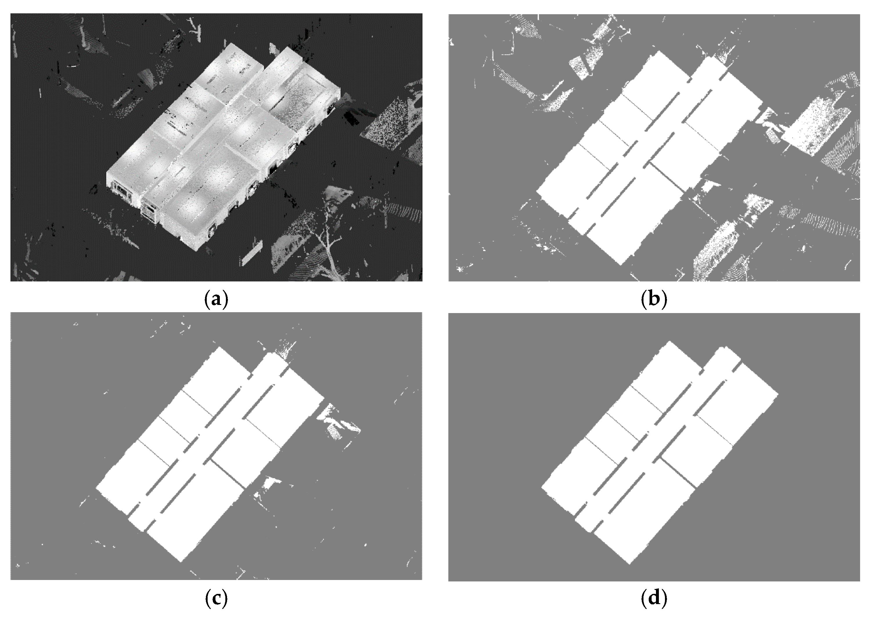
Figure 3a provides an example of raw point-cloud input, and Figure 3b demonstrates its projection onto the 2D binary map, wherein the occupied pixels in white represent the indoor environments of the building or noise, and the unoccupied pixels in gray represent the outside environments of building or walls. Figure 3b also shows the problem presented by noisy pixels when projecting the entire point-cloud acquisition. Noisy pixels occur when projecting the scan points that pass through windows. To prevent any possible problems with the later morphological processing, it is desirable to remove these points rather than keeping them as occupied pixels in the binary map. To that end, only the points within the ceiling and floor height intervals (the two peaks in Figure 2) are kept for rasterization. Then, in order not to miss any structural details, an offset space from the ceiling height interval is defined, as illustrated in Figure 4, in order to add points within it into the rasterization. This is valid, because vertical walls are as high as the ceiling height, while most clutter and windows are rather less than the ceiling height [10]. The offset space from the floor is not considered, because clutter near the floor is more hindrance than help. In this way, the unwanted scan points outside the building can be greatly reduced and cut off from the main segment, as shown in Figure 3c. After rasterization, we perform a labeling process to remove any pixel segments that do not belong to the main segment. In this process, the algorithm defines which pixels are connected to other pixels based on the number of connected neighborhoods (4-connectivity was assumed in the present study). Each connected segment is uniquely labeled with different integer values, and its pixels are counted [12,36]. Among the labeled segments, the largest one is retained; the others, considered to be noise, are removed. Figure 3d shows the rasterized point cloud after noise filtering.
3.4. Initial Segmentation
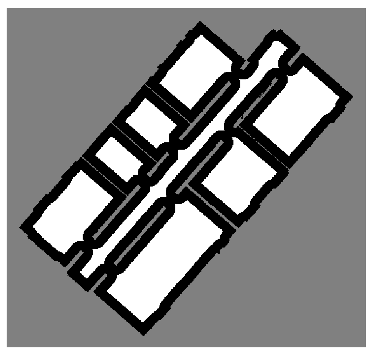
Given the noise-filtered binary map, an initial segment map is created to roughly locate single rooms. The initial segment map plays an important role in that it determines the number of rooms to be segmented and also provides a starting point for detailed segmentation of each room. Assuming that different rooms and corridors are connected by narrow passages such as doorways, the user needs to define a detection window greater than the largest doorway. This detection window visits all of the occupied pixels on the binary map and counts the number of unoccupied pixels within its range. If the count is zero, which indicates that the center of the detection window is farther from the nearby walls than its range, the algorithm classifies the center pixel as a part of the initial segments; otherwise, the center pixel is classified as a part of unsegmented areas. Note that a circular-shaped detection window is desirable, because the sharp corners of other, polygonal-shaped detection windows easily bump into the boundaries of a narrow hallway, thus often failing to create the correct initial segment map. By moving the detection window onto all of the occupied pixels one by one, the original binary map is partitioned into several isolated regions, as shown in Figure 5. Each isolated region in white represents a single room consisting of homogeneous, occupied pixels. The black areas are the occupied, but unsegmented pixels to be segmented in the later phases, and the gray areas are the unoccupied pixels, such as walls or outside building environments, that do not need to be segmented.
3.5. Opening Closure
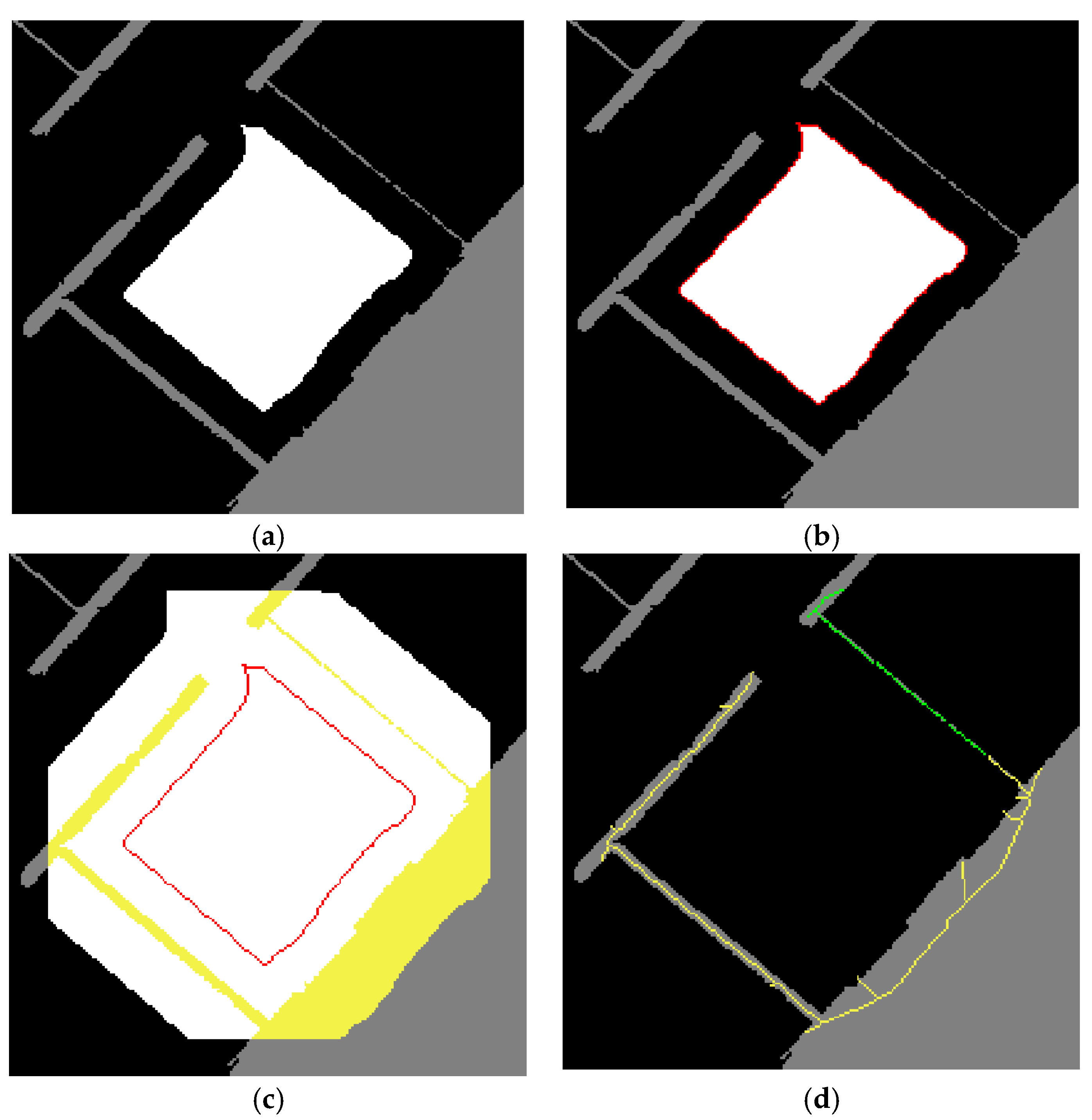
This section describes in detail the main contribution of our paper: a method for creation of the watertight floor map from the initial segmentation using the morphological process illustrated in Figure 6. In this study, we define a room as a region bound by vertical walls and linked to other rooms through doorway openings. The key operation is the separation of a room from the others by closing all of the openings to them. The algorithm begins by selecting one segment (Figure 7a) from the initial segment map, and finds the surrounding walls (unoccupied pixels) to be closed. For that purpose, a 1-pixel-thick boundary of the selected initial segment is traced as shown in Figure 7b. Then, a new detection window is defined to find the surrounding walls: it visits all of the occupied pixels composing the boundary and finds any unoccupied pixels within its range. This time, the size of the detection window is double that specified in the initial segmentation phase so as to find all of the surrounding walls without exception. Additionally, a square-shaped detection window is desirable, because it is advantageous to include a sharp corner. The surrounding walls are represented in yellow in Figure 7c, which includes a doorway and other small openings. Note that small openings are found when the pixel size is not sufficiently smaller than the minimum wall thickness; in order to prevent hollow parts in a low-point-density area, sometimes this is unavoidable. These openings are closed by iteratively connecting the closest pixels of two different wall segments. To reduce the computation loads for finding the closest pixels, a skeletonization algorithm is adopted. The algorithm iteratively reduces pixels composing an object in a binary map to retain a skeletal remnant that has the same distance from two closest pixels on the object boundary [37]. The skeletonized image yields a 1-pixel-thick center line that preserves the topology of the original walls while reducing the search space for finding the closest pixels. The resulting skeleton, due to the openings, is often divided into several small skeletons, one of which is labeled yellow and the others green, as shown in Figure 7d.
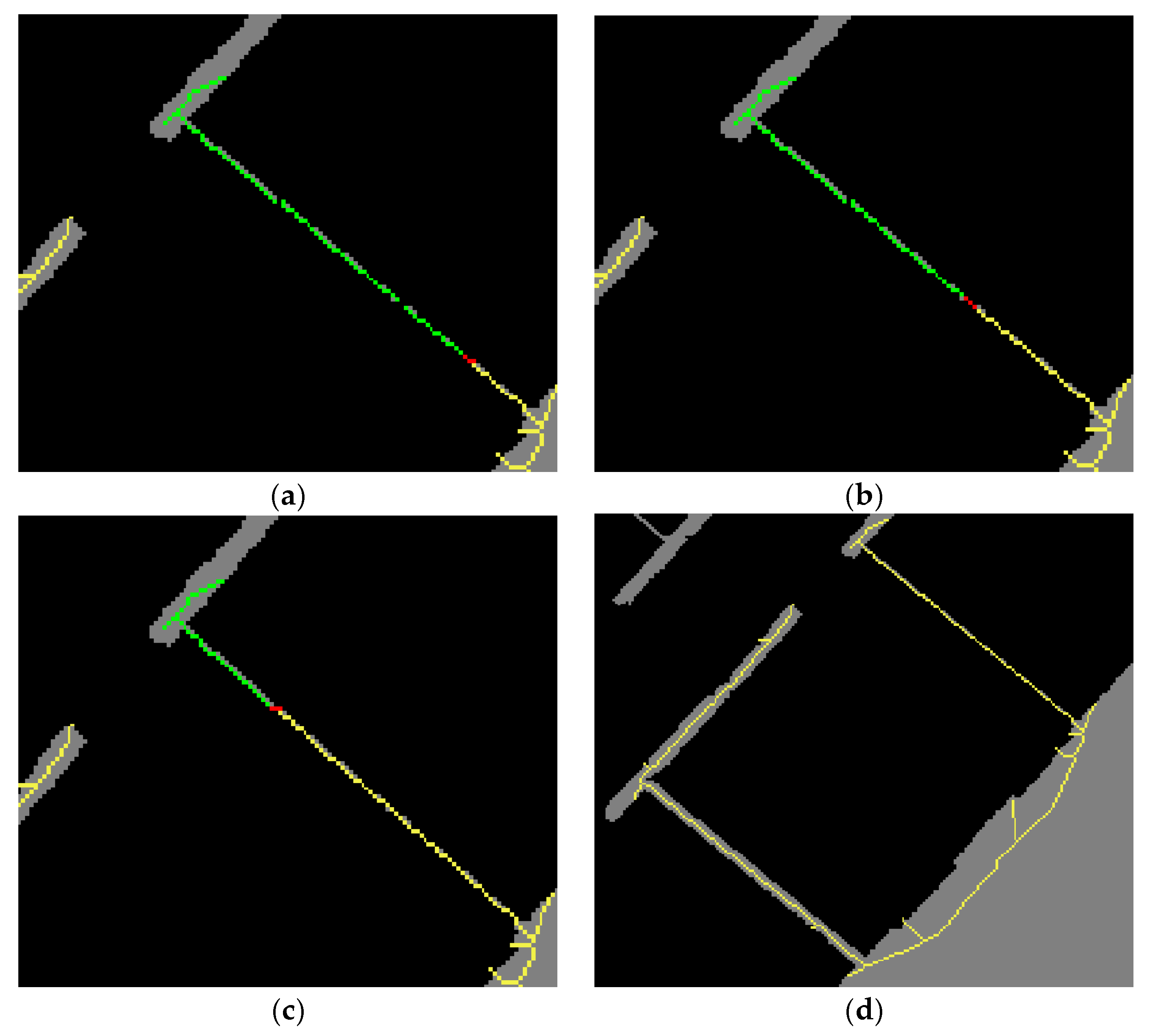
The two closest pixels are determined by computing the distances of all pixel-to-pixel combinations between two groups; see, for example, the yellow skeleton and the other, green skeletons in Figure 7d. The point pair with the shortest distance is determined by Equation (1),
where is the pixel pair with the shortest distance; and are the pixels from two different pixel groups, respectively; and and are the numbers of pixels composing the respective skeletons. A 1-pixel-thick line (the red pixels in Figure 8a), which is intersected by the straight line connecting the closest two pixels, is found by Bresenham’s algorithm [38] and used to close the opening. Then, both of the connected green skeletons and the 1-pixel-thick red line are combined with the yellow skeleton. This process operates recursively until all of the green skeletons are combined with the yellow skeleton (Figure 8b,c). Note that this iterative process is skipped if the skeletonized wall initially has only one opening or none. At the final iteration, all of the skeletonized walls are combined to form a single skeleton, which inevitably leaves one last opening to be closed (Figure 8d).
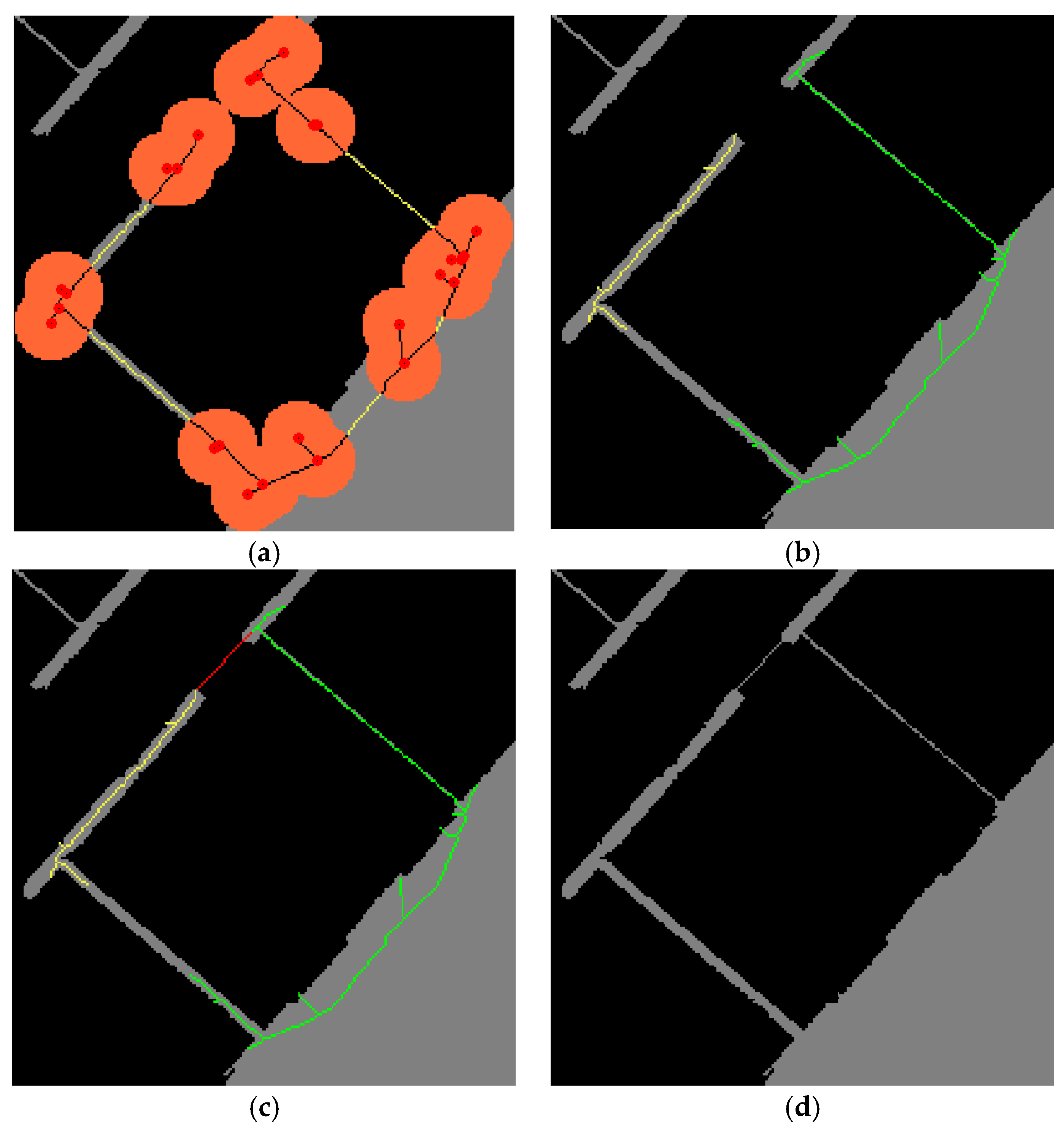
This problem is resolved by temporarily creating a new larger opening than the previous one, which enables finding the closest pixels in the last opening. Note that the new opening should be located on the main branch of the skeleton tree; otherwise, the closest two pixels will be found in the new opening, not in the last opening. The above-noted conditions can be achieved by removing all of the small branches. To that end, all of the end pixels and junctions of the last skeleton are found and excluded together with their nearby skeleton pixels within the range of a new detection window whose size and shape are the same as those of the window used in the rasterization phase. This is valid, because the small branches of the last skeleton cannot be greater than half the detection window size. As a result, in the example of Figure 9a, the single skeleton is temporarily broken into five smaller skeletons (yellow lines), the longest of which is selected for the temporary opening. In Figure 9b, the original skeleton is broken again into two smaller skeletons (green and yellow) by the temporary opening, which allows for finding of the two closest pixels in the last opening by computing the shortest distance, as shown in Figure 9c. Finally, the temporary opening is restored back to the wall, resulting in the closed room shown in Figure 9d. The entire process is repeated until all of the surrounding walls of each initial segment are completely closed to create a watertight floor map, on which, in the next phase, each room can be segmented by a labeling process.
3.6. Room Labeling and Refinement
A labeling process is performed on the generated watertight floor map to separate rooms from each other. In the labeling process, each connected segment is uniquely labeled and sorted according to the occupied pixel count. The number of top largest segments, which are supposed to be classified as rooms, is determined by the initial segmentation phase. Typically, the other remaining segments do not include a sufficient number of occupied pixels to be classified as individual rooms, and thus should be reclassified among the above-classified rooms. Likewise, the occupied pixels used for closing the openings (red pixels in Figure 8 and Figure 9) should also be classified. In the refinement phase, we investigate all of the eight-connectivity neighboring pixels of those occupied but unclassified segments, and group the neighboring pixels according to their labels. The dominant label is determined by counting the number of occupied pixels of each group, and is then used to label the unclassified segments. The refinement process operates recursively until no other unclassified segments are found. Examples before and after application of refinement are illustrated in Figure 10, where the unclassified segments in black are classified as green according to the dominant label of the neighboring pixels.
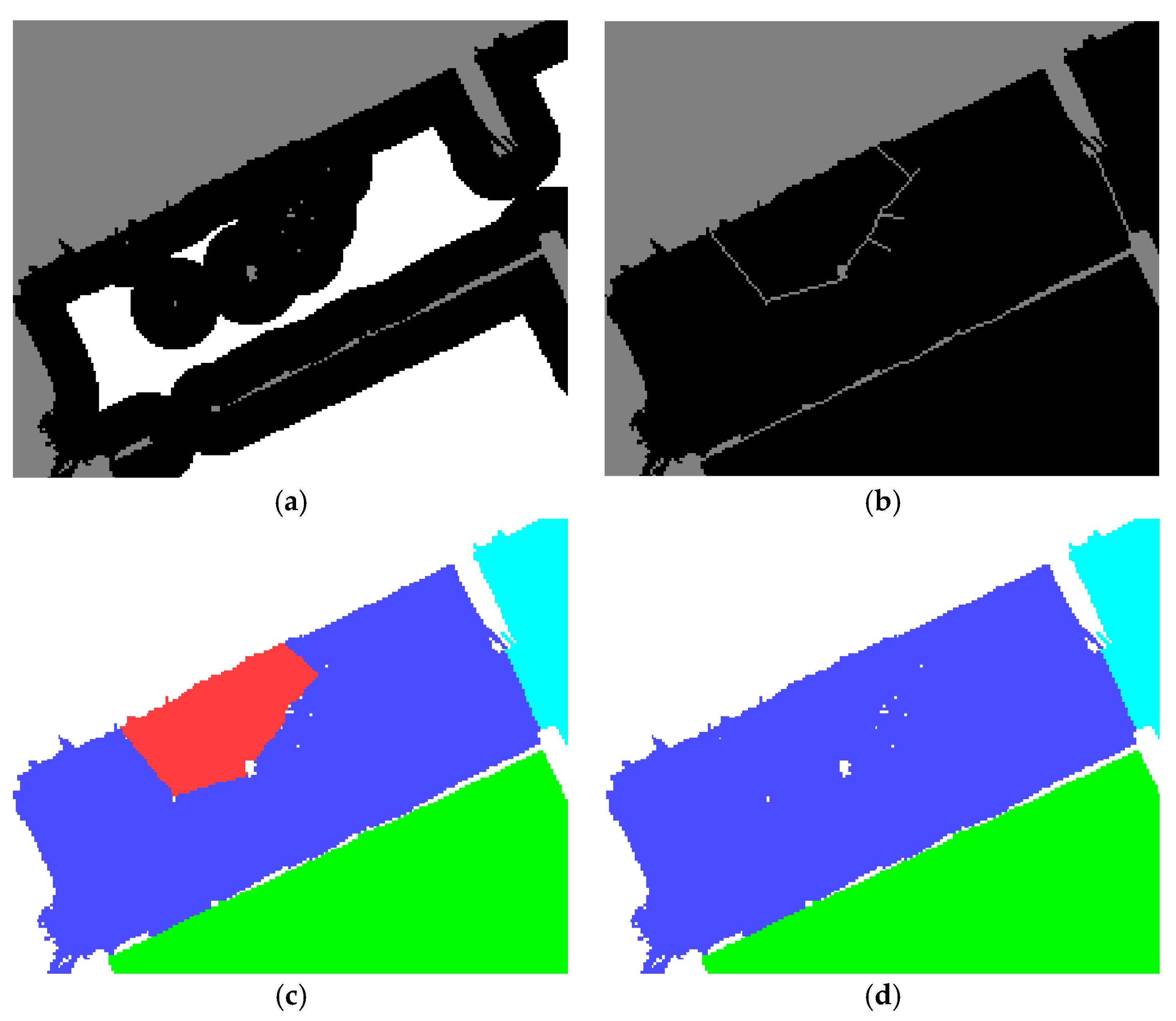
Over-segmentation can occur when the initial segmentation incorrectly finds single rooms due to hollow parts on the rasterized point cloud. The main factors leading to hollow parts are the presence of low-density areas or unfiltered occlusions. Typically, low-density areas can be prevented either by selecting the proper pixel size for rasterization or by performing multiple scans. However, significant clutter passing through the ceiling and floor, such as stairs, columns, or pipelines, inevitably produces hollow parts on the rasterized binary map. Since hollow parts sometimes are identified as walls (unoccupied pixels), as shown in Figure 11a, they can lead to over-segmentation, as shown in Figure 11b,c. To address this problem, we investigate all of the eight-connectivity neighboring pixels of individual rooms, and classify them as occupied or unoccupied. If the number of occupied pixels is greater than the number of unoccupied pixels, indicating that more than half of the neighboring pixels are occupied by the other rooms, which would be against our assumption that a room is a region bounded by walls (i.e., unoccupied pixels), the current room is reclassified among the other rooms according to the dominant label (Figure 11d). This process operates recursively until all of the individual rooms are tested, thus creating the final segment map. Subsequently, the original 3D scan points are segmented according to their projected 2D locations on the final segment map.
4. Experiments and Results
4.1. Evaluation with Real-World Data Sets
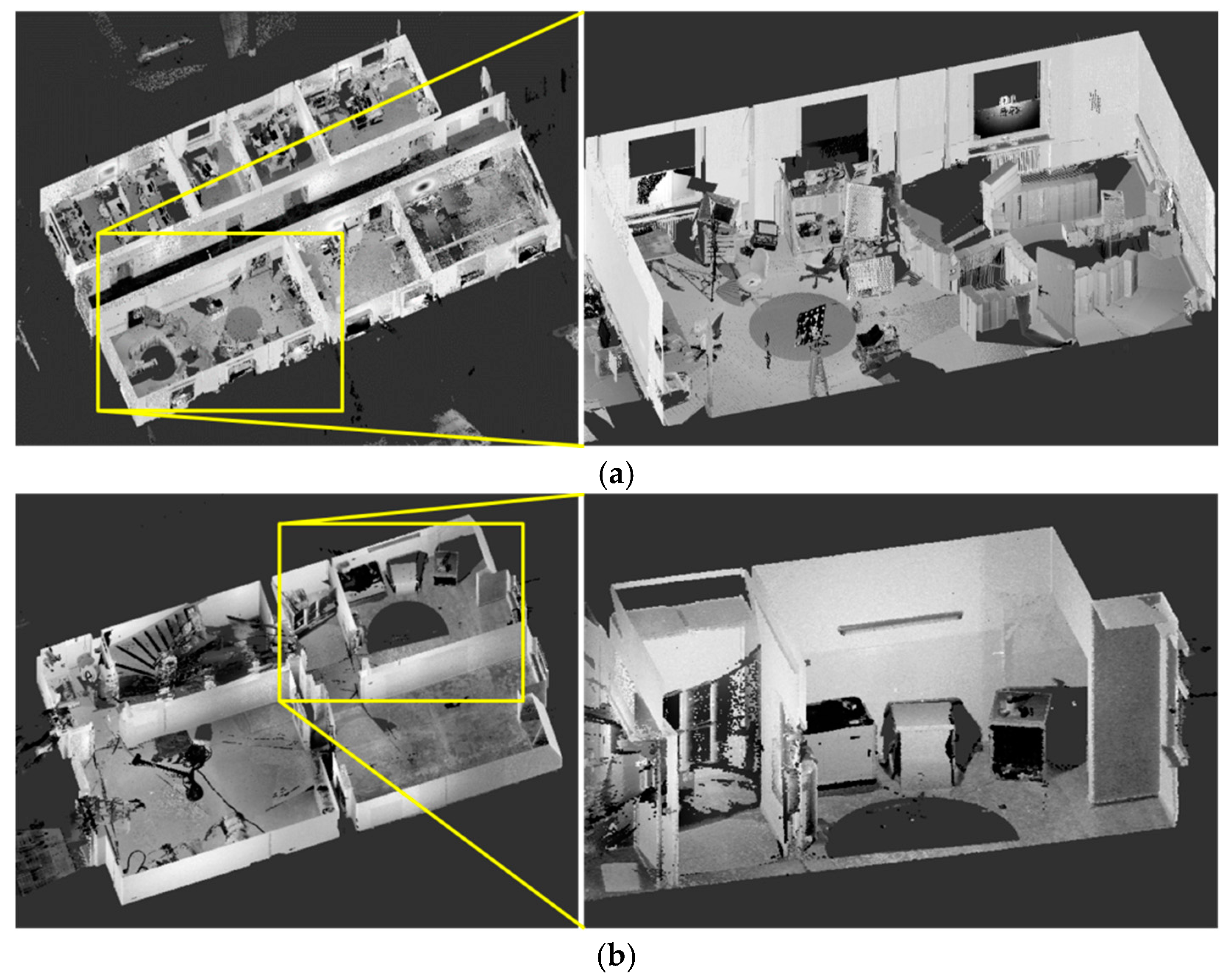
We evaluated the proposed approach using two real-world data sets acquired by a phase-based laser scanner, FARO Focus 3D. The first data set contained approximately 66 million scan points, including a long corridor that connects seven rooms. The second data set contained approximately 31 million scan points, including five rooms and stairs ascending into the upper floor. The scanning results for these sites, as representative of severe occlusions and clutter, are illustrated in Figure 12. We implemented the proposed room segmentation approach in MATLAB for prototyping, and performed the experiment on a laptop computer with Intel Core i7 (2.3 GHz, 16.0 GB of RAM).
The test parameters are listed in Table 2. Except for parameter selection, our approach is automatic and does not require any user intervention. In the height estimation phase, considering the distance accuracy of the laser scanner (±2 mm for Focus 3D), a sufficiently large height interval of 0.1 m was adopted for both data sets to effectively detect the points constituting the ceiling and floor in the histogram. In the noise filtering phase, to properly remove the noisy points while preserving the structural detail, the offset value should be slightly less than the distance between the ceiling and the highest points of openings or furniture. In this study, the distance was measured to 0.56 m for the first data set and to 0.45 m for the second data set; accordingly, the offset values of 0.5 and 0.4 m were adopted for the first and the second data sets, respectively. Note that these offset spaces were our subjective choices; certainly, one could alter or skip this process to extend the segmentation capabilities. For rasterization, a large pixel size can reduce processing time, but a too-large pixel size incurs large distortions in wall boundaries. By contrast, a small pixel size preserves the precise boundaries, but a too-small pixel size greatly increases processing time and can lead to hollow parts for low-density areas. Therefore, the pixel size should be smaller than the size of the detectable wall thickness, but should not be too small to prevent hollow parts on the binary map. In this study, the pixel sizes of 0.05 and 0.03 m were adopted for the first and the second data sets, respectively, resulting in binary maps of 459 by 446 pixels for the first data set and 203 by 249 pixels for the second.
The rasterization phase requires, for initial segmentation, one additional parameter: the detection window size. A large detection window size increases the number of pixels to be investigated within its range, thus requiring excessive processing time. In addition, a large detection window size does not necessarily equate to better performance; in fact, the detection window size is recommended to be just slightly greater than the existing openings. In practice, the user is required to define the radius of the detection window; as for the diameter of the detection window for initial segmentation (Table 2), it is determined by doubling the radius and adding one pixel size representing the detection window center. By contrast, the other two detection window sizes in the opening-closure phase are automatically determined according to the first detection window size in the rasterization phase.
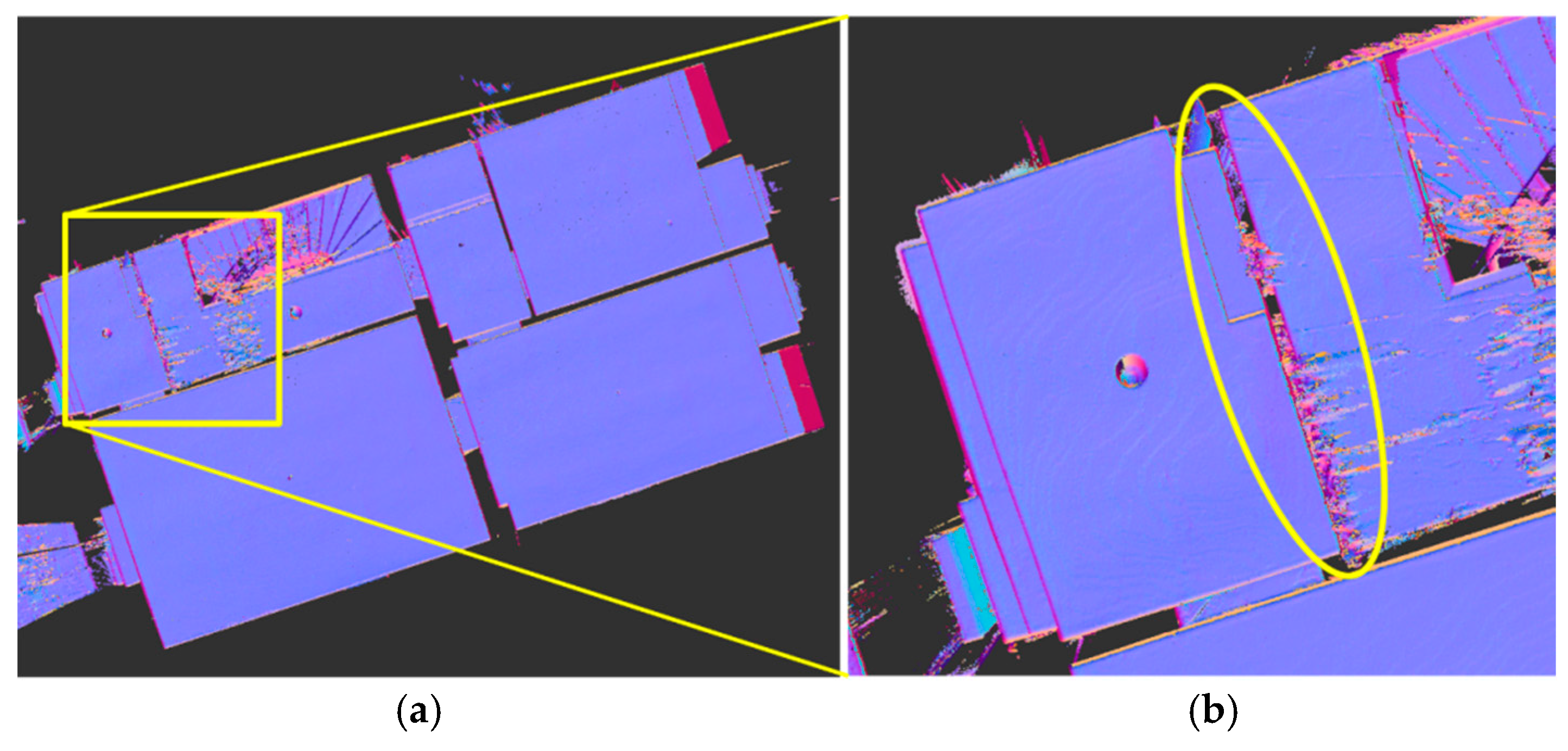
Figure 13a,b shows the generated segment maps for the first and second real-world data sets, respectively. The total time consumption was 22.27 s for the first data set and 16.78 s for the second. Then, the original 3D points were segmented, as shown in Figure 13c,d, according to their projected 2D locations on the segment maps. As is apparent, the proposed approach performed well with the first real-world data set. Note that some holes in the blue point cloud were due to occlusions by furniture at the time of scanning. In the second data-set result, however, we encountered a problem, which is that the algorithm, as shown in Figure 14a, failed to decompose the first segment into two different rooms. The main factor leading to this incorrect segmentation was the noisy scan points that filled the empty space between two wall surfaces as shown in Figure 14b, and which were projected onto the binary map and segmented together with the other (correctly) occupied pixels. The diffused noisy points were mainly due to a mirror in the scan area [39]. To enhance the current noise-filtering phase, one possible means would be planar detection [40], which will be the focus of one of our future studies.
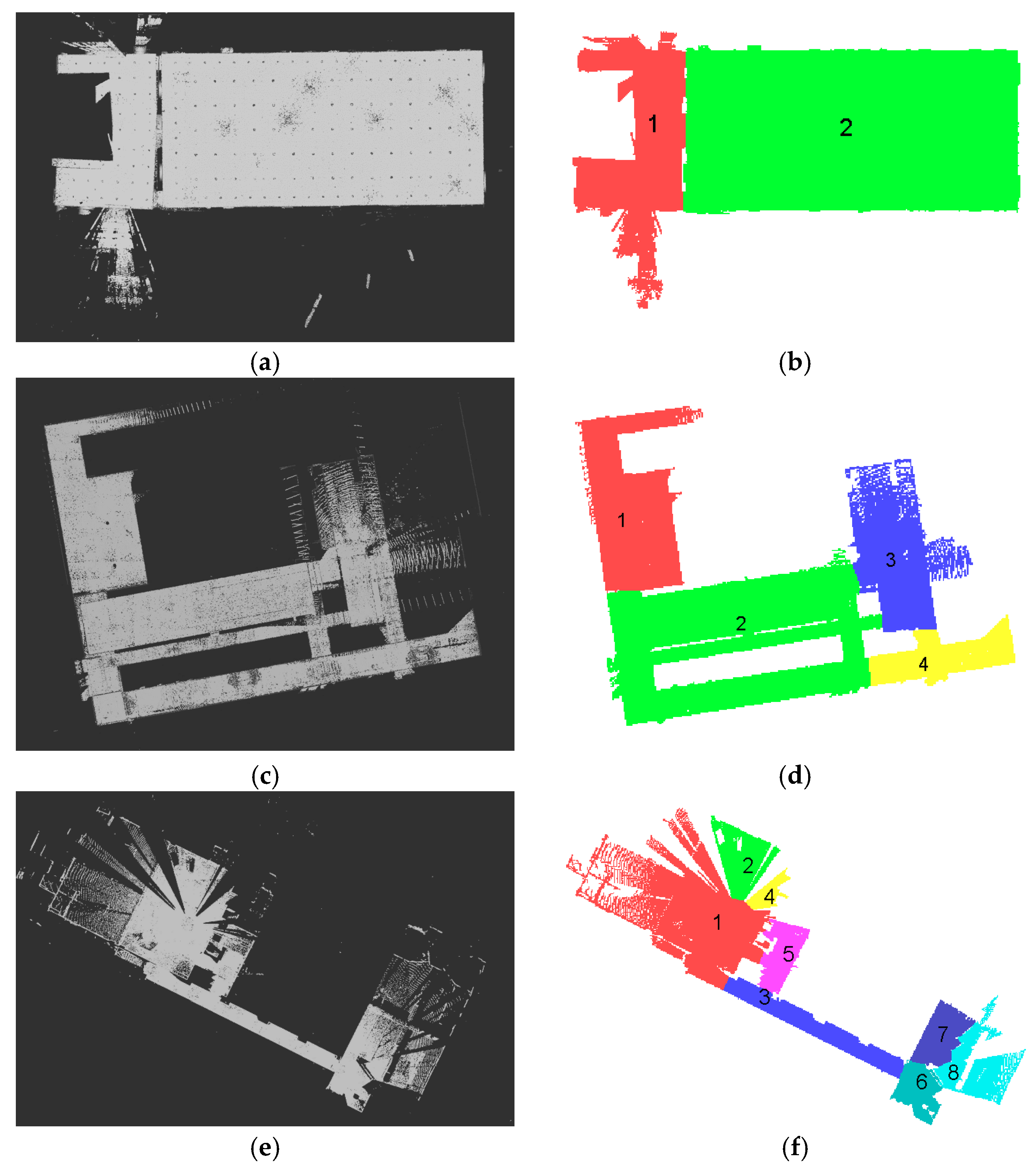
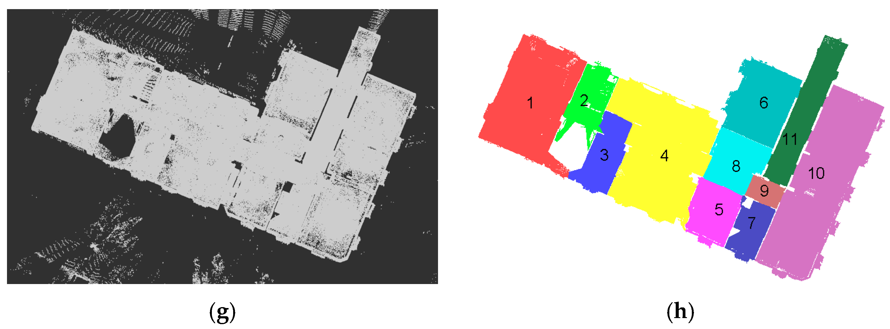
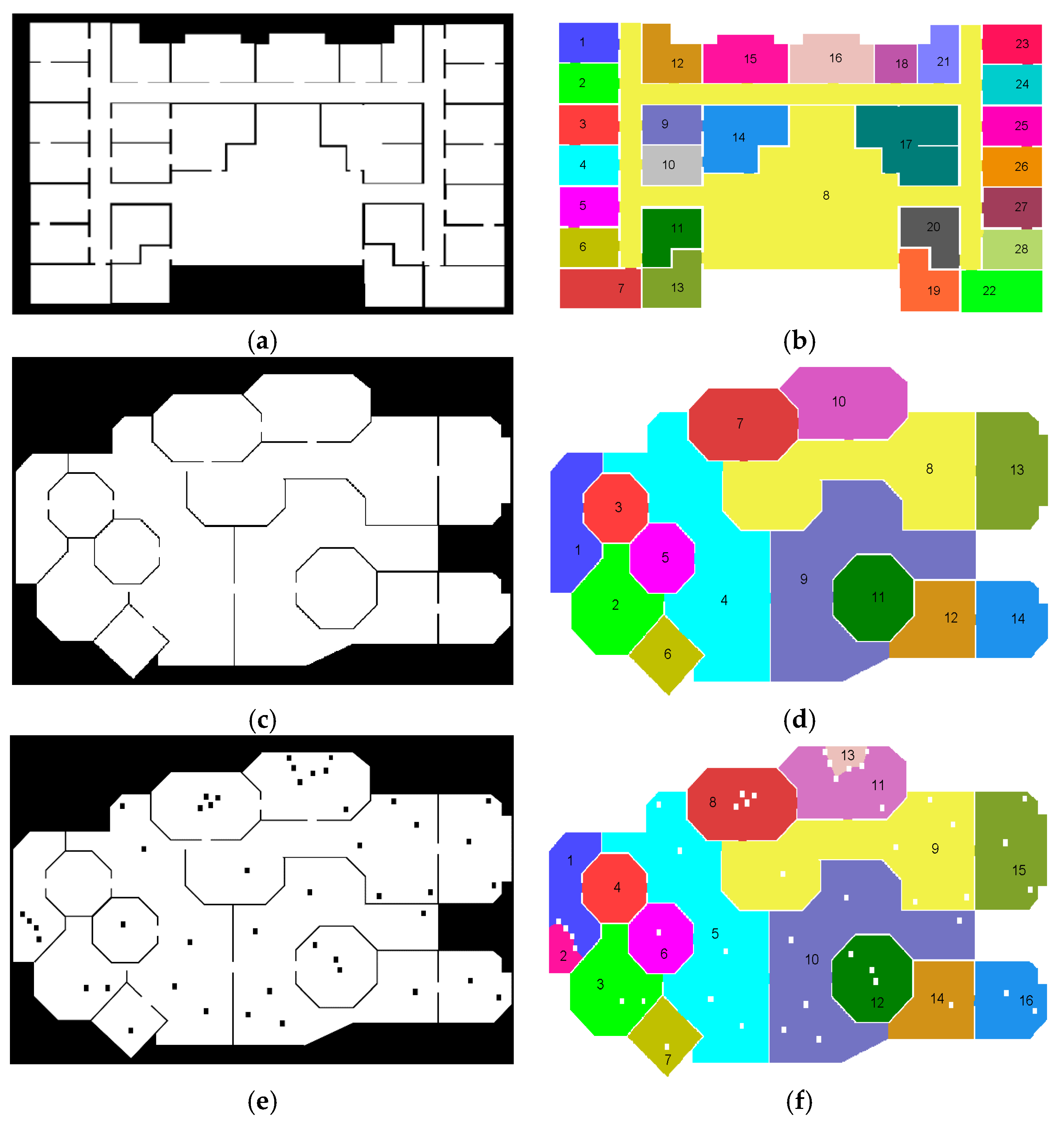
Additionally, we evaluated our room segmentation approach, as shown in Figure 15, using four publicly available point-cloud data sets [41]. The details of the experiments are summarized in Table 3. For each data set, the pixel sizes were selected so as to be smaller than the size of the detectable wall thickness, but not too small to prevent hollow parts on the binary map. For the initial segmentation, meanwhile, the detection window sizes were selected to be greater than the existing openings measured in the point cloud. The height estimation and noise-filtering offset were not considered in the experiments with the publicly available data sets, due to the different ceiling levels of the rooms. Compared with the above-mentioned two real-world data sets, the publicly available data sets were more challenging, due to the complicated architectural shapes and incomplete scans. Nevertheless, the segment maps yielded generally good results for separation of rooms with straight segment boundaries. In Figure 15a, the first publicly available data set is a relatively simple structure, and its two rooms were correctly segmented by the proposed approach, as shown in Figure 15b. With the second data set in Figure 15c, the algorithm successfully separated the small segments (room numbers 1, 3, and 4 in Figure 15d) from the main hall (room number 2 in Figure 15d), but failed to decompose the main hall into a room and a corridor. This was due to the fact that the corridor violated one of our assumptions (i.e., two different regions are connected with narrower passages): it was directly connected to the other rooms without doorways, and thus the algorithm failed to create proper initial segments. On the other hand, with the third data set in Figure 15e, the algorithm over-produced the segments (room numbers 1, 2, and 4; and 6, 7, and 8 in Figure 15f) due to the hollow parts stemming from incomplete scans. To avoid this problem, meticulous scanning without spaces is required so as to minimize occluded areas. However, for cases in which sufficient scanning is not available, an effective refinement strategy will be taken into consideration in future work. Finally, as indicated in Figure 15g,h, the algorithm yielded overall good agreements with the experimental data. Note though that due to the small pixel size and the greater number of rooms, the processing time was longer than for the other data sets. The several factors affecting processing time will be discussed in detail in the following section.
4.2. Evaluation with Synthetic Data Sets
In order to check the feasibility of the proposed approach for the data sets with nonlinear architectural shapes and larger numbers of rooms, we generated five synthetic floor plans. Note that all of the tests were directly performed on the 2D binary map. In Figure 16a, the first binary map includes the greatest number of rooms connected by a long corridor that makes a large loop, but its overall architectural shape is relatively simple, consisting of rectangular-shaped rooms. In Figure 16c, the second binary map is still limited to straight boundaries, but the architectural shape is more complicated than the first one. In Figure 16e, the third binary map has the same architectural shape as the second one, but includes many hollow parts for consideration of scan holes due to low-density areas or tall furniture reaching to the ceiling level. In Figure 16g, the fourth binary map includes some nonlinear architectural shapes and small openings. Finally, the fifth binary map in Figure 16i shows the most complicated case among the synthetic data sets: the architectural shape is described by a set of highly nonlinear boundaries. Notably, each room on all of the synthetic binary maps includes one or more openings to other rooms.
The detailed test specifications are listed in Table 4. Note that the time consumption does not include point-cloud rasterization. Table 4 indicates that the time consumption is influenced by four factors: number of rooms, hollow parts, and the map and detection window sizes in the rasterization phase. A larger number of rooms (data set 1) and hollow parts (data set 3) undoubtedly incur more time consumption, because they increase the number of openings to be investigated. Likewise, a large map size certainly increases the time consumption. Since the map size is determined by the pixel size in the rasterization phase, users need to select the proper pixel size for minimization of the computational loads but preservation of the precise architectural shapes; we recommend the use of half the minimum wall thickness. In this test, the pixel size of 5 cm was assumed for all of the synthetic binary maps. The detection window size greatly influences the processing time; for example, the segmentation of data set 4 became much more time consuming even with the smallest number of rooms. As we discussed above, a large detection window size does not necessarily equate to better performance. Therefore, a smaller detection window size is to be preferred, as long as it provides for proper initial segmentation.
The resultant segment maps are compared with the input binary maps in Figure 16. Overall, the proposed approach was proved to be not susceptible to either the number of rooms or complex architectural shapes. However, in Figure 16f, compared with Figure 16d, two regions (room numbers 2 and 13) were found to be over-segmented. This problem was due to the fact that several hollow parts prevented the detection window from entering those rooms, thus leading to incorrect initial segmentation. In the refinement phase, if the number of neighboring, unoccupied pixels of a segment is greater than the number of occupied ones, the algorithm is not able to distinguish the over-segmented room from the other, real rooms. To prevent hollow parts on the binary map, users need to either select a greater pixel size for rasterization or perform multiple scans to avoid low-density areas.
4.3. Comparison with Existing Methods Using Publicly Available Data Sets
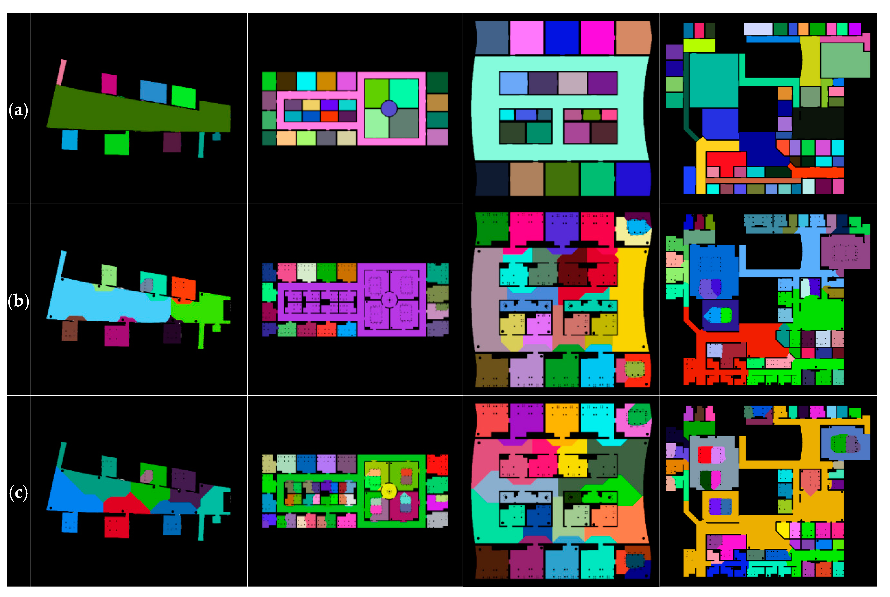
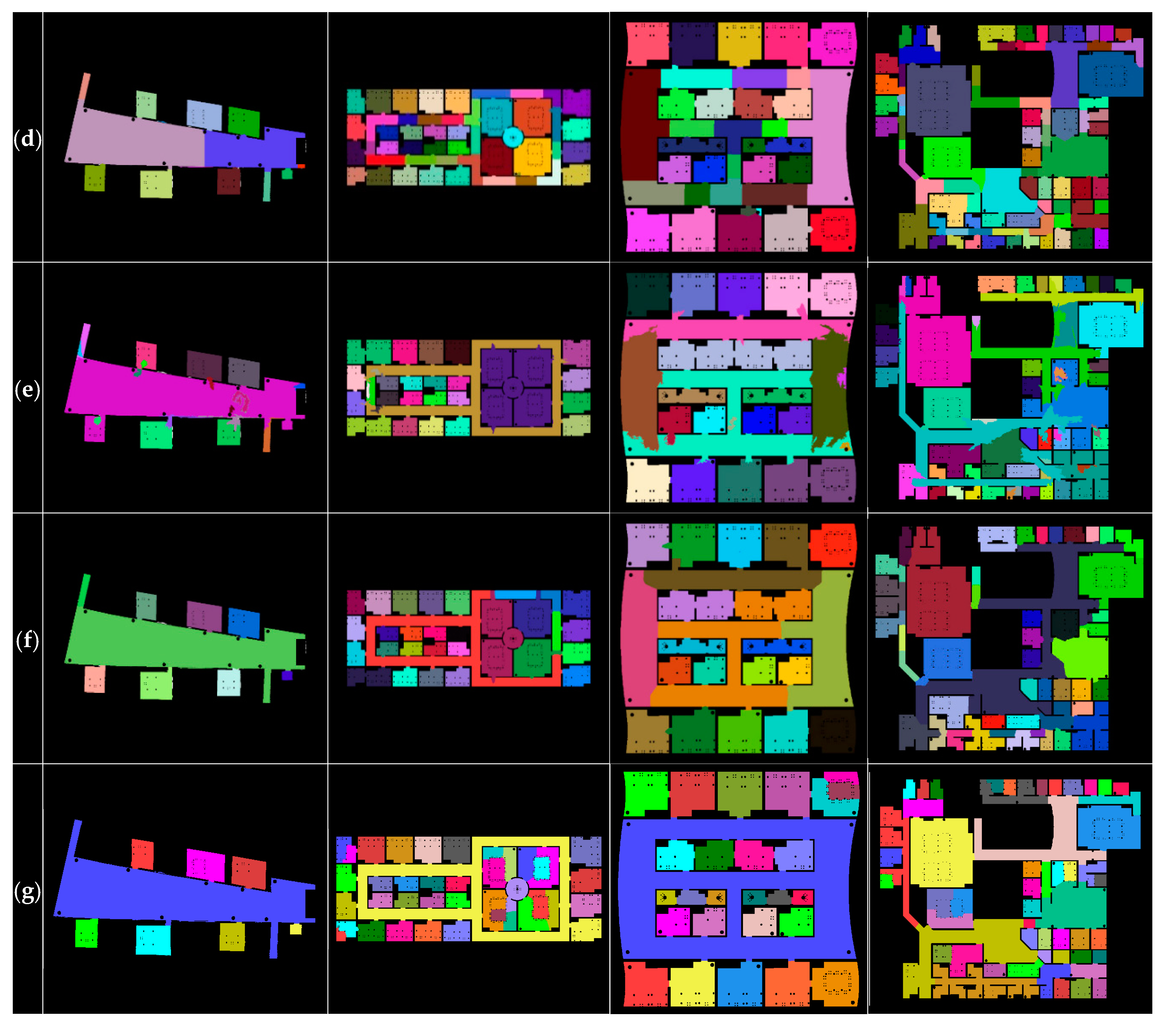
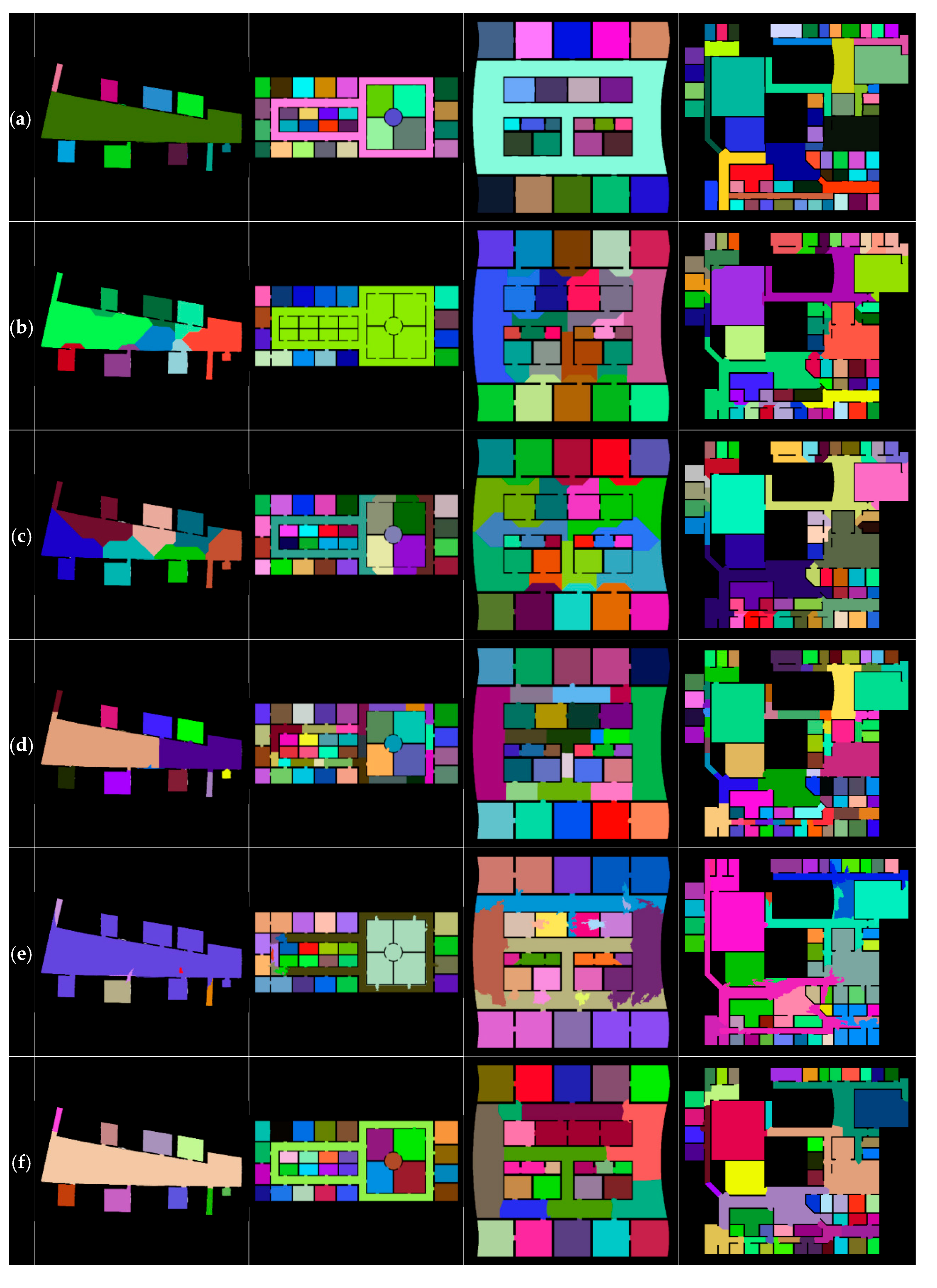
Additionally, we compared our room segmentation with those of five popular existing methods using 20 publicly available non-furnished data sets [19]. Use of these data sets reflected our assumption that occlusions and clutter are properly reduced by means of point-cloud projection. Figure 17 provides a visual comparison of the segment maps created by each of the algorithms. Due to the length limit of this paper, only four segmentation results, those that best describe the strengths and limitations of the proposed approach, are listed in the figure. Figure 17a–g depicts the ground truths by human segmentation, the morphological segmentation [22], the distance transform-based segmentation [23], the Voronoi graph-based segmentation [20], the feature-based segmentation [33], the Voronoi random field segmentation [34], and our room segmentation, respectively.
At this stage, one should note that we used the existing ground truths and segmentation results available online [42] to avoid any subjectivities and ambiguities arising from reproducing the segment maps with different test specifications and parameter adjustments.
Overall, the existing methods offer irregular or ragged segments, and are susceptible to severe over- or under-segmentation. As indicated in Figure 17b, the morphological approach resulted in highly ragged segmentations with the first, third, and fourth data sets, and showed severe under-segmentation with the second data set (the brown-colored regions). Likewise, the distance transform-based approach (Figure 17c) suffered from arbitrarily segmented boundaries over the test data sets. The Voronoi graph-based approach (Figure 17d) enabled straight segment boundaries, but severe over-segmentation was found for the long corridor in the second data set and on the main hall in the third data set. The feature-based approach (Figure 17e) showed the worst results: highly ragged boundaries and severe under-segmentation over the test data sets. Among the existing methods, the Voronoi random field approach (Figure 17f) generated the best overall segmentation results, though over-segmentation with ragged boundaries was still an issue, as shown for the third test data set. With regard to Figure 17g, visual inspection suggested that our approach has distinct advantages over the existing methods: it is resistant to over- or under-segmentation, and provides straight segment boundaries. More specifically, compared with the ground truths, our approach yielded quite similar segmented rooms and corridors for the second and third data sets. For the first and fourth data sets, our approach also afforded satisfactory results in the separation of rooms, but tended to some under- or over-segmentation of corridors. For example, with the first data set in Figure 17g, the two narrow corridors in the upper-left and lower-right corners were not properly separated from the main hall because, as is the case in Figure 15e, they violated our second assumption (i.e., two different regions are connected with narrower passages). The fourth data set, as shown in Figure 17g, contained several different-sized passages; thus, in the initial segmentation phase, some corridors could not be properly separated by means of a single detection window size.
Meanwhile, occlusions and clutter on occupancy grid maps cannot be avoided, as they are often generated from the 2D horizontal sensor readings at the height just above the floor. Given this reality, experiments with 20 publicly available furnished data sets were additionally performed. Figure 18 provides a visual comparison of just four of those sets (due to the paper-length limit) using manual segmentation (Figure 18a), morphological segmentation (Figure 18b), distance transform-based segmentation (Figure 18c), Voronoi graph-based segmentation (Figure 18d), feature-based segmentation (Figure 18e), Voronoi random field segmentation (Figure 18f), and our room segmentation (Figure 18g) method. The ground truths and segmentation results with the furnished data are available online [42]. In the segmentation results, the occlusions due to furniture yielded no sensor readings for grid mapping, and thus remained as unsegmented black areas. Overall, compared with the experimental results with the non-furnished data, the existing methods resulted in more severe over-segmentation even with very simple test data. Our approach yielded similar results for the first and third data sets, but tended to over-segmentation for the second and fourth sets. This was attributable to the inability of the detection window in the initial segmentation phase to pass through the areas where there were lots of occlusions, thus resulting in over-production of the initial segments.
Finally, quantitative evaluations are carried out using three different measures: correctness, completeness, and absolute deviation [40,43]. The correctness and completeness measures were calculated pixel-by-pixel in comparing the automatically segmented map with the ground truths. In Equation (2), the correctness measure evaluates the percentage of the matched pixels among the automatically detected ones. On the other hand, the completeness measure in Equation (3) provides the percentage of the matched pixels among the manually detected ones (i.e., the ground truths). Lastly, the absolute deviation is the absolute difference between the number of rooms detected manually () and the number of rooms detected automatically (). This measure indicates the robustness against over- or under-segmentations. Table 5 lists the evaluation metrics computed by the five existing methods and our approach using the 20 publicly available data sets without and with furniture.
In the table, the average values indicate the average measures of the five existing methods. Each bolded value is a best or second-best result. Overall, it was found that the proposed approach outperformed all of the average values. In the case of the non-furnished data sets, the correctness of the proposed approach (89.6 ± 9.8%) was comparable with the second-best value (90.0 ± 8.4%) achieved by the Voronoi-random method. Moreover, the proposed approach achieved the best results for the measures of completeness (91.7 ± 9.0%) and absolute-deviation (2.5). Meanwhile, in the case of the furnished data sets, the proposed approach achieved two second-best results, for the measures of correctness and completeness (84.8 ± 13.9% and 67.8 ± 14.5%), respectively, which proved that the proposed room segmentation is an effective approach for furnished environments.
5. Conclusions
In the AEC industry, recently, the demand for as-built BIM creation of large and complex building interiors has increased with the advent of high-performance laser scanning devices. However, automated and detail-rich as-built modeling remains a challenge, as the available commercial and academic tools require excessive processing time and manual work. One way to facilitate the Scan-to-BIM process is to obtain a separate point cloud for each room, which allows for effective operation of the modeling phases for each room while reducing the computational complexity as compared with processing the entire data set. Such room segmentation is necessary for creating topological relationships to enrich 3D models with semantic information of the sort that is required for BIM. Unfortunately, most existing methods utilized in the AEC community rely on strict constraints or known scanner locations, a fact that limits their applications to specific data sets. Meanwhile, within the robotics community, room segmentation usually has been implemented on occupancy grid maps in a 2D context, which often leads to over-segmentation with arbitrarily segmented boundaries.
In contrast to the conventional methods, our input is just a registered point cloud acquired by either a static laser scanner or a mobile scanning system; supplementary data, such as known scanner locations or training data, are not needed for the segmentation, thus allowing for more general applications of the proposed approach, even to existing or publicly available data. Based on the assumption that each room is bound by vertical walls, we propose to project the 3D point-cloud input onto a 2D binary map and to segment rooms using morphological processing. We tested our approach under a variety of data conditions, including real-world, synthetic, and publicly available 2D and 3D data sets. The experiments with the real-world data sets demonstrated the robustness against occlusions and clutter in 3D point clouds, while the experiments with the five synthetic data sets proved our method’s high segmentation performance regardless of the number of rooms or the complexity of architectural shapes. Additionally, comparisons with the five popular existing methods were conducted using 20 publicly available non-furnished and furnished data sets. The qualitative evaluations proved that the proposed approach is resistant to over- or under-segmentation while preserving straight segment boundaries. In the quantitative evaluations, the proposed approach exceeded the existing methods in terms of the measures of completeness and absolute deviation with non-furnished data, and the measures of correctness and completeness with furnished data.
Overall, the proposed approach achieved high performance with the non-furnished data sets. It also had relatively good results when dealing with the furnished data sets, although improvement in this area is necessary. It can also be a problem when only parts of a building are scanned, as shown in Figure 15. Thus, in future work, we will further investigate occlusion problems to improve the robustness of our method against such furnished or incomplete data input. In addition, we will aim at automatic detection window size control allowing for segmentation of complex indoor environments containing several different-sized passages. Although the proposed noise filtering helps to reduce the number of unwanted scan points outside the building, noise inside the scan area remains a problem that leads to the type of segmentation failure indicated in Figure 14. Therefore, other means of resolving this problem will be considered, for example, the removal of noisy points that are beyond a certain range from nearby walls extracted by planar detection. Based on the segmented point cloud, the next phase of our research will involve segmentation and modeling of detail-rich architectural components, such as columns, windows, and doors, for as-built BIM creation.
Acknowledgments
This research was supported by the Basic Science Research Program through the National Research Foundation of Korea (NRF) funded by the Ministry of Education (2015R1A6A3A03019594).
Author Contributions
Jaehoon Jung developed the main program, and wrote most of the paper. Cyrill Stachniss contributed to the data collection, and provided comments. Corresponding author Changjae Kim provided guidance throughout the course of the research.
Conflicts of Interest
The authors declare no conflict of interest.
References
- Bosche, F.N.; O’Keeffe, S. The Need for Convergence of BIM and 3D Imaging in the Open World. In Proceedings of the CitA BIM Gathering Conference, Dublin, Ireland, 12–13 November 2015; pp. 109–116. [Google Scholar]
- Xiong, X.; Adan, A.; Akinci, B.; Huber, D. Automatic creation of semantically rich 3D building models from laser scanner data. Autom. Constr. 2013, 31, 325–337. [Google Scholar] [CrossRef]
- Tang, P.; Huber, D.; Akinci, B.; Lipman, R.; Lytle, A. Automatic reconstruction of as-built building information models from laser-scanned point clouds: A review of related techniques. Autom. Constr. 2010, 19, 829–843. [Google Scholar] [CrossRef]
- Carbonari, G.; Stravoravdis, S.; Gausden, C. Building information model implementation for existing buildings for facilities management: A framework and two case studies. In Building Information Modelling (BIM) in Design, Construction and Operations; WIT Press: Southampton, UK, 2015; Volume 149, pp. 395–406. [Google Scholar]
- Wang, C.; Cho, Y.K. Application of As-built Data in Building Retrofit Decision Making Process. Procedia Eng. 2015, 118, 902–908. [Google Scholar] [CrossRef]
- Randall, T. Construction Engineering Requirements for Integrating Laser Scanning Technology and Building Information Modeling. J. Constr. Eng. Manag. 2011, 137, 797–805. [Google Scholar] [CrossRef]
- Jung, J.; Hong, S.; Yoon, S.; Kim, J.; Heo, J. Automated 3D Wireframe Modeling of Indoor Structures from Point Clouds Using Constrained Least-Squares Adjustment for As-Built BIM. J. Comput. Civ. Eng. 2016, 30, 04015074. [Google Scholar] [CrossRef]
- Valero, E.; Adan, A.; Cerrada, C. Automatic Method for Building Indoor Boundary Models from Dense Point Clouds Collected by Laser Scanners. Sensors 2012, 12, 16099–16115. [Google Scholar] [CrossRef] [PubMed]
- Hong, S.; Jung, J.; Kim, S.; Cho, H.; Lee, J.; Heo, J. Semi-automated approach to indoor mapping for 3D as-built building information modeling. Comput. Environ. Urban Syst. 2015, 51, 34–46. [Google Scholar] [CrossRef]
- Previtali, M.; Barazzetti, L.; Brumana, R.; Scaioni, M. Towards automatic indoor reconstruction of cluttered building rooms from point clouds. In Proceedings of the ISPRS Technical Commission V Symposium, Riva del Garda, Italy, 23–25 June 2014; Volume 2, pp. 281–288. [Google Scholar]
- Thomson, C.; Boehm, J. Automatic Geometry Generation from Point Clouds for BIM. Remote Sens. 2015, 7, 11753–11775. [Google Scholar] [CrossRef]
- Jung, J.; Hong, S.; Jeong, S.; Kim, S.; Cho, H.; Hong, S.; Heo, J. Productive modeling for development of as-built BIM of existing indoor structures. Autom. Constr. 2014, 42, 68–77. [Google Scholar] [CrossRef]
- Budroni, A.; Böhm, J. Automatic 3D modelling of indoor Manhattan-world scenes from laser data. In Proceedings of the ISPRS Commission V Mid-Term Symposium ‘Close Range Image Measurement Techniques’, Newcastle upon Tyne, UK, 21–24 June 2010; Volume 38, pp. 115–120. [Google Scholar]
- Adán, A.; Huber, D. Reconstruction of Wall Surfaces under Occlusion and Clutter in 3D Indoor Environments; Robotics Institute, Carnegie Mellon University: Pittsburgh, PA, USA, 2010. [Google Scholar]
- Mura, C.; Mattausch, O.; Villanueva, A.J.; Gobbetti, E.; Pajarola, R. Automatic room detection and reconstruction in cluttered indoor environments with complex room layouts. Comput. Graph. 2014, 44, 20–32. [Google Scholar] [CrossRef]
- Ochmann, S.; Vock, R.; Wessel, R.; Klein, R. Automatic reconstruction of parametric building models from indoor point clouds. Comput. Graph. 2016, 54, 94–103. [Google Scholar] [CrossRef]
- Turner, E.L. 3D Modeling of Interior Building Environments and Objects from Noisy Sensor Suites. Ph.D. Thesis, The University of California, Berkeley, CA, USA, 14 May 2015. [Google Scholar]
- Macher, H.; Landes, T.; Grussenmeyer, P. Point clouds segmentation as base for as-built BIM creation. In Proceedings of the 25th International CIPA Symposium, Taipei, Taiwan, 31 August–5 September 2015; Volume 2, pp. 191–197. [Google Scholar]
- Bormann, R.; Jordan, F.; Li, W.; Hampp, J.; Hagele, M. Room Segmentation: Survey, Implementation, and Analysis. In Proceedings of the IEEE International Conference on Robotics and Automation, Stockholm, Sweden, 16–21 May 2016; pp. 1019–1026. [Google Scholar]
- Wurm, K.M.; Stachniss, C.; Burgard, W. Coordinated multi-robot exploration using a segmentation of the environment. In Proceedings of the IEEE International Conference on Intelligent Robots and Systems, Nice, France, 22–26 September 2008; pp. 1160–1165. [Google Scholar]
- Mozos, Ó.M.; Stachniss, C.; Rottmann, A.; Burgard, W. Using adaboost for place labeling and topological map building. In Robotics Research; Springer: Berlin, Germany, 2007; Volume 28, pp. 453–472. [Google Scholar]
- Fabrizi, E.; Saffiotti, A. Augmenting topology-based maps with geometric information. Robot. Auton. Syst. 2002, 40, 91–97. [Google Scholar] [CrossRef]
- Diosi, A.; Taylor, G.; Kleeman, L. Interactive SLAM using laser and advanced sonar. In Proceedings of the IEEE International Conference on Robotics and Automation, Barcelona, Spain, 18–22 April 2005; pp. 1103–1108. [Google Scholar]
- Jebari, I.; Bazeille, S.; Battesti, E.; Tekaya, H.; Klein, M.; Tapus, A.; Filliat, D.; Meyer, C.; Ieng, S.-H.; Benosman, R.; et al. Multi-sensor semantic mapping and exploration of indoor environments. In Proceedings of the 3rd IEEE Incernational Conference on Technologies for Practical Robot Applications, Woburn, MA, USA, 11–12 April 2011; pp. 151–156. [Google Scholar]
- Brunskill, E.; Kollar, T.; Roy, N. Topological mapping using spectral clustering and classification. In Proceedings of the IEEE International Conference on Intelligent Robots and Systems, San Diego, CA, USA, 29 October–2 Novermber 2007; pp. 3491–3496. [Google Scholar]
- Shi, L.; Kodagoda, S.; Ranasinghe, R. Fast indoor scene classification using 3D point clouds. In Proceedings of the Australasian Conference on Robotics and Automation, Melbourne, Australia, 7–9 December 2011; pp. 1–7. [Google Scholar]
- Siemiatkowska, B.; Harasymowicz-Boggio, B.; Chechlinski, Ł. Semantic Place Labeling Method. J. Autom. Mob. Robot. Intell. Syst. 2015, 9, 28–33. [Google Scholar] [CrossRef]
- Burgard, W.; Fox, D.; Hennig, D.; Schmidt, T. Estimating the absolute position of a mobile robot using position probability grids. In Proceedings of the 13th National Conference on Artificial Intelligence, Portland, OR, USA, 4–8 August 1996; pp. 896–901. [Google Scholar]
- Lu, Z.; Hu, Z.; Uchimura, K. SLAM estimation in dynamic outdoor environments: A review. In Proceedings of the 2nd International Conference on Intelligent Robotics and Applications, Singapore, 16–18 December 2009; pp. 255–267. [Google Scholar]
- Ochmann, S.; Vock, R.; Wessel, R.; Tamke, M.; Klein, R. Automatic generation of structural building descriptions from 3D point cloud scans. In Proceedings of the 9th IEEE International Conference on Computer Graphics Theory and Applications, Lisbon, Portugal, 5–8 January 2014; pp. 1–8. [Google Scholar]
- Ikehata, S.; Yang, H.; Furukawa, Y. Structured indoor modeling. In Proceedings of the IEEE International Conference on Computer Vision, Santiago, Chile, 13–16 December 2015; pp. 1323–1331. [Google Scholar]
- Meinel, G.; Neubert, M. A comparison of segmentation programs for high resolution remote sensing data. Int. Arch. Photogramm. Remote Sens. 2004, 35 Pt B, 1097–1105. [Google Scholar]
- Mozos, O.M.; Rottmann, A.; Triebel, R.; Jensfelt, P.; Burgard, W. Semantic labeling of places using information extracted from laser and vision sensor data. In Proceedings of the IEEE International Conference on Intelligent Robots and Systems, Beijing, China, 9–15 October 2006. [Google Scholar]
- Friedman, S.; Pasula, H.; Fox, D. Voronoi Random Fields: Extracting Topological Structure of Indoor Environments via Place Labeling. In Proceedings of the 20th International Joint Conference on Artificial Intelligence, Hyderabad, India, 9–12 January 2007; Volume 7, pp. 2109–2114. [Google Scholar]
- Li, Y.; Hu, Q.; Wu, M.; Liu, J.; Wu, X. Extraction and Simplification of Building Façade Pieces from Mobile Laser Scanner Point Clouds for 3D Street View Services. ISPRS Int. J. Geo-Inf. 2016, 5, 231. [Google Scholar] [CrossRef]
- Motameni, H.; Norouzi, M.; Jahandar, M.; Hatami, A. Labeling method in Steganography. Int. Sch. Sci. Res. Innov. 2007, 1, 1600–1605. [Google Scholar]
- Han, S.; Cho, H.; Kim, S.; Jung, J.; Heo, J. Automated and efficient method for extraction of tunnel cross sections using terrestrial laser scanned data. J. Comput. Civ. Eng. 2012, 27, 274–281. [Google Scholar] [CrossRef]
- Bresenham, J.E. Algorithm for computer control of a digital plotter. IBM Syst. J. 1965, 4, 25–30. [Google Scholar] [CrossRef]
- Käshammer, P.; Nüchter, A. Mirror identification and correction of 3D point clouds. Int. Arch. Photogramm. Remote Sens. Spat. Inf. Sci. 2015, 40, 109. [Google Scholar] [CrossRef]
- Kim, C.; Habib, A.; Pyeon, M.; Kwon, G.-R.; Jung, J.; Heo, J. Segmentation of Planar Surfaces from Laser Scanning Data Using the Magnitude of Normal Position Vector for Adaptive Neighborhoods. Sensors 2016, 16, 140. [Google Scholar] [CrossRef] [PubMed]
- DURAARK Datasets. Available online: http://duraark.eu/data-repository/ (accessed on 22 June 2017).
- IPA Room Segmentation. Available online: http://wiki.ros.org/ipa_room_segmentation (accessed on 12 February 2017).
- Rodríguez-Cuenca, B.; García-Cortés, S.; Ordóñez, C.; Alonso, M.C. Morphological operations to extract urban curbs in 3D MLS point clouds. ISPRS Int. J. Geo-Inf. 2016, 5, 93. [Google Scholar] [CrossRef]
Figure 1.
Schematization of proposed room segmentation.
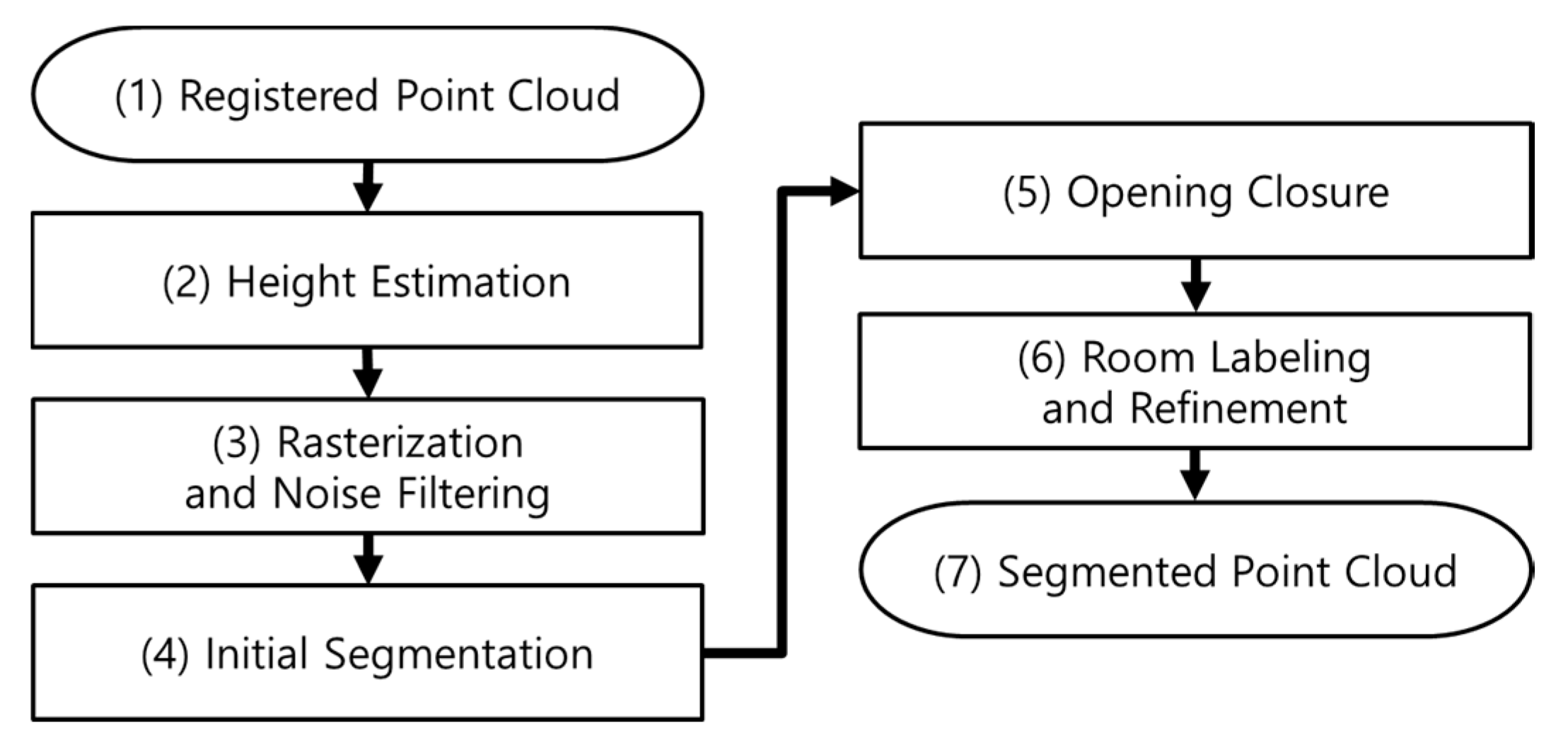
Figure 2.
Histogram representing number of scan points according to variation of height.
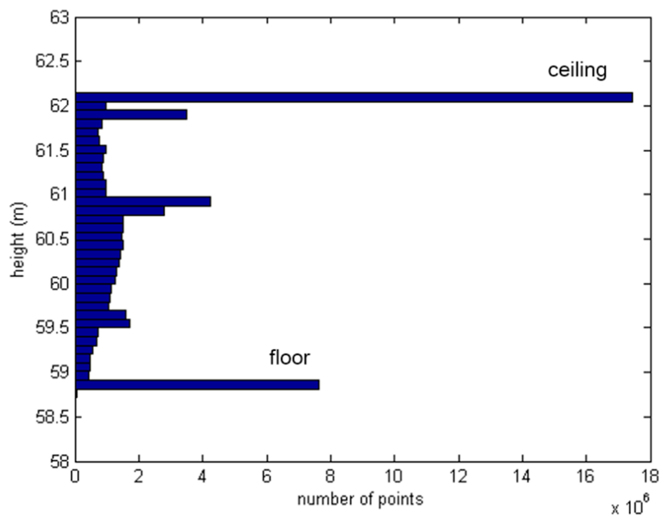
Figure 3.
Rasterization of point cloud: (a) raw point-cloud input; (b) rasterization of raw point-cloud input; (c) rasterization after reducing noisy points passing through windows; and (d) main segment filtered by labeling process.
Figure 3.
Rasterization of point cloud: (a) raw point-cloud input; (b) rasterization of raw point-cloud input; (c) rasterization after reducing noisy points passing through windows; and (d) main segment filtered by labeling process.

Figure 4.
Offset space for noise filtering process.
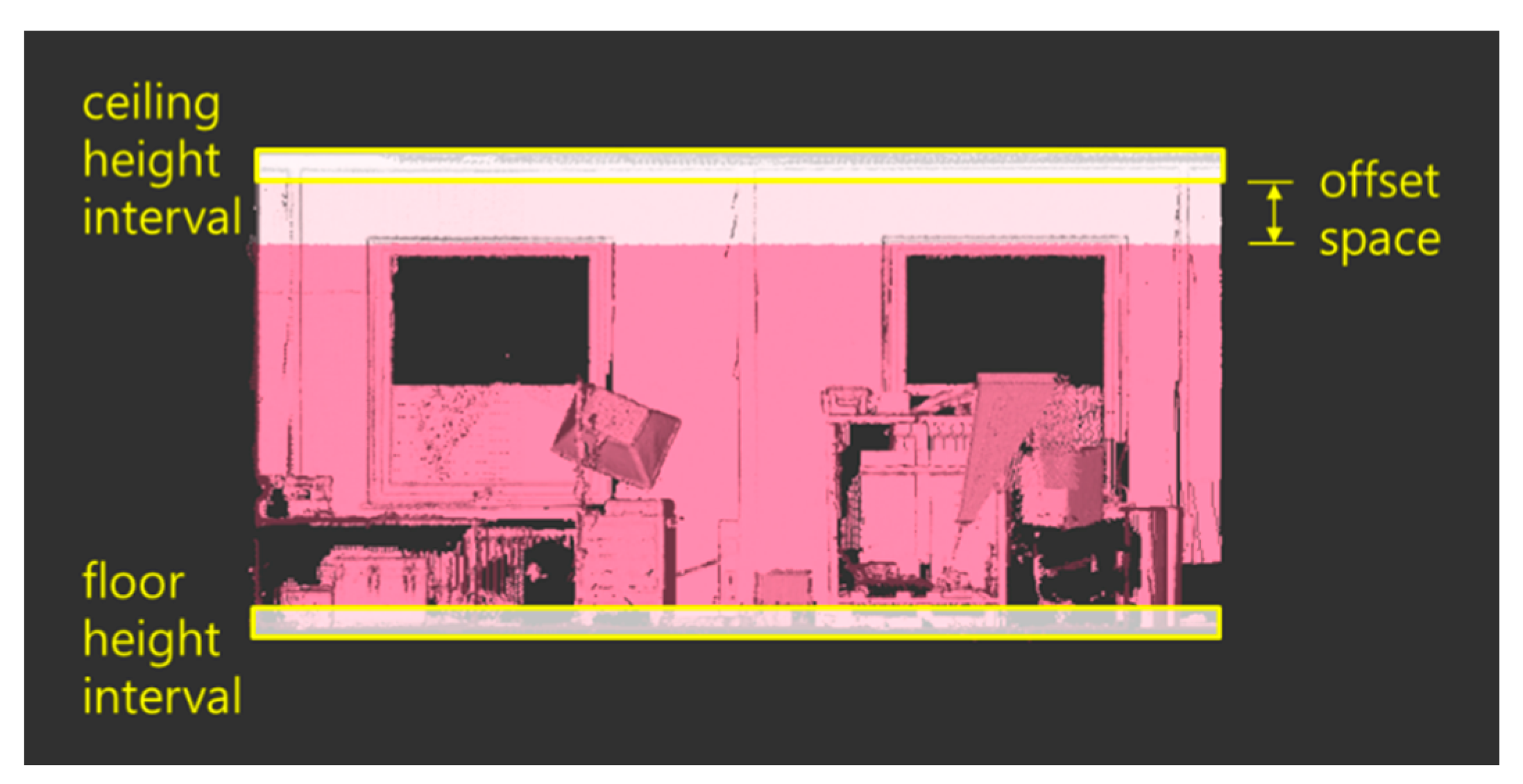
Figure 5.
Initial segment map creation.

Figure 6.
Procedure for opening closure.
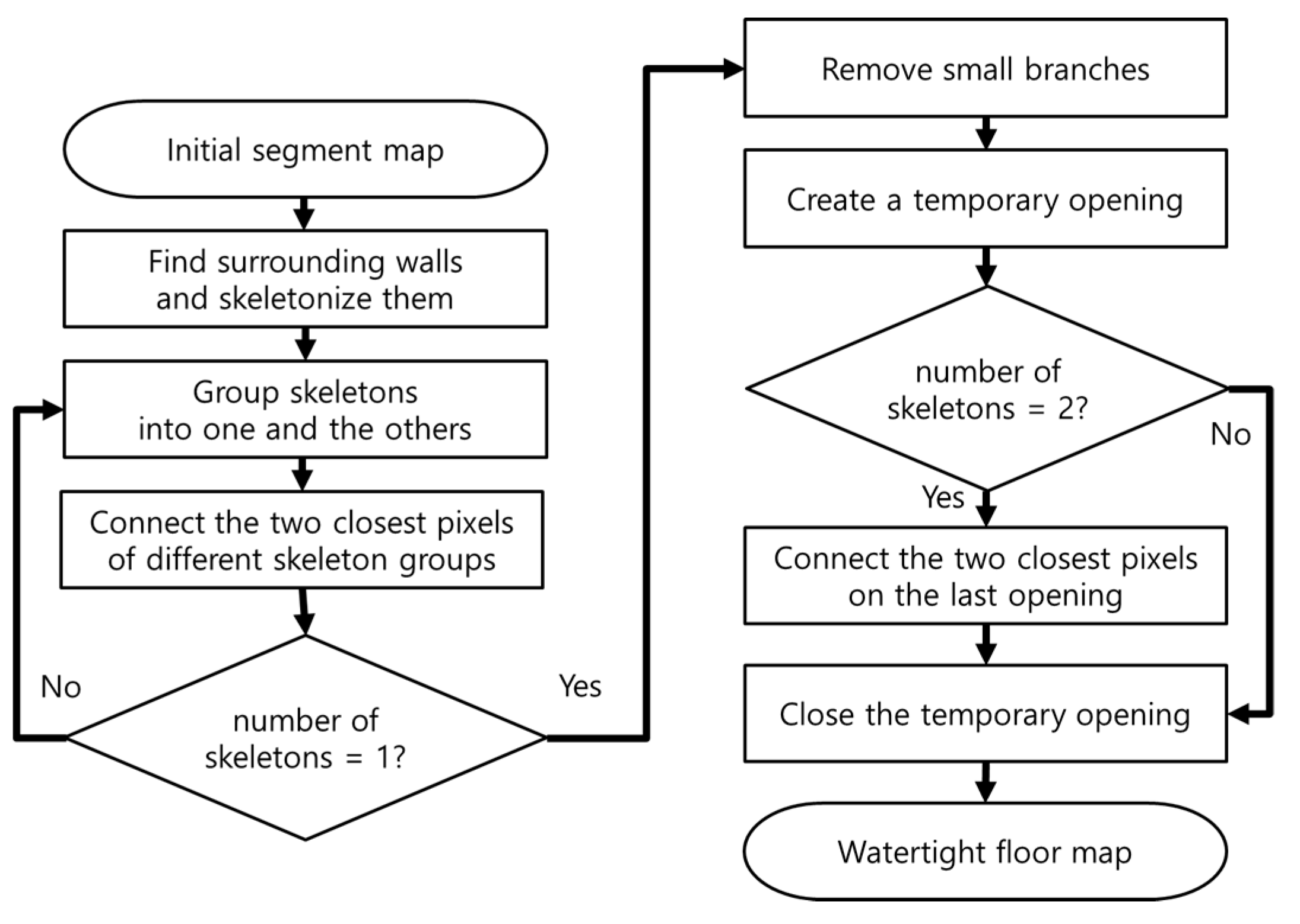
Figure 7.
Process of wall detection: (a) selection of one initial segment; (b) boundary tracing; (c) detection; and (d) skeletonization of surrounding walls.
Figure 7.
Process of wall detection: (a) selection of one initial segment; (b) boundary tracing; (c) detection; and (d) skeletonization of surrounding walls.

Figure 8.
Example of opening closure: (a–c) openings on skeletonized walls are sequentially found and closed; and (d) all skeletonized walls are combined to form a single skeleton.
Figure 8.
Example of opening closure: (a–c) openings on skeletonized walls are sequentially found and closed; and (d) all skeletonized walls are combined to form a single skeleton.

Figure 9.
Closure of last opening: (a) removal of small branches on skeleton tree; (b) creation of temporary opening; (c) finding of two closest pixels in last opening and their closure; and (d) formation of watertight room.
Figure 9.
Closure of last opening: (a) removal of small branches on skeleton tree; (b) creation of temporary opening; (c) finding of two closest pixels in last opening and their closure; and (d) formation of watertight room.

Figure 10.
Example of refinement for unclassified segments colored in black: (a) before; and (b) after refinement.
Figure 10.
Example of refinement for unclassified segments colored in black: (a) before; and (b) after refinement.
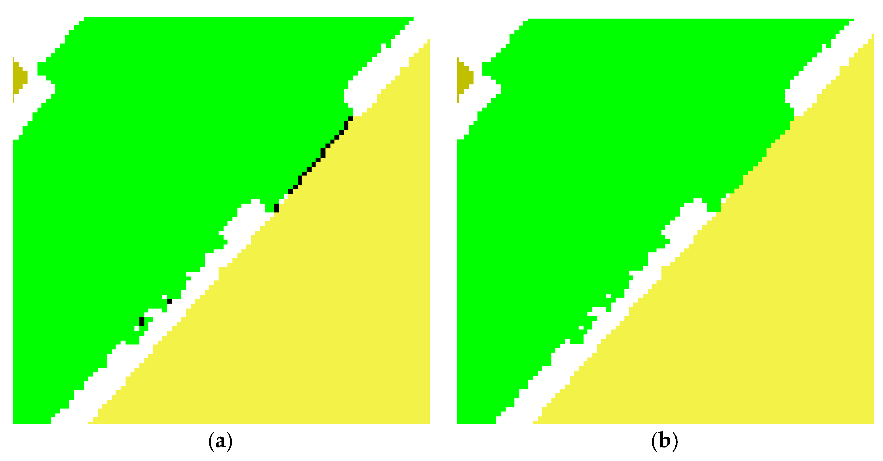
Figure 11.
Example of refinement process for over-segmentation: (a–c) incorrect segmentation due to hollow parts; and (d) merging of over-segmented room (colored in red) into nearby room (colored in blue).
Figure 11.
Example of refinement process for over-segmentation: (a–c) incorrect segmentation due to hollow parts; and (d) merging of over-segmented room (colored in red) into nearby room (colored in blue).

Figure 12.
Point-cloud Input: first (a); and second (b) data sets, representing severe occlusion and clutter. Ceiling points are omitted for clarity.
Figure 12.
Point-cloud Input: first (a); and second (b) data sets, representing severe occlusion and clutter. Ceiling points are omitted for clarity.

Figure 13.
Segmentation results for two real-world data sets: (a,b) 2D segment maps; and (c,d) 3D segmented point clouds.
Figure 13.
Segmentation results for two real-world data sets: (a,b) 2D segment maps; and (c,d) 3D segmented point clouds.
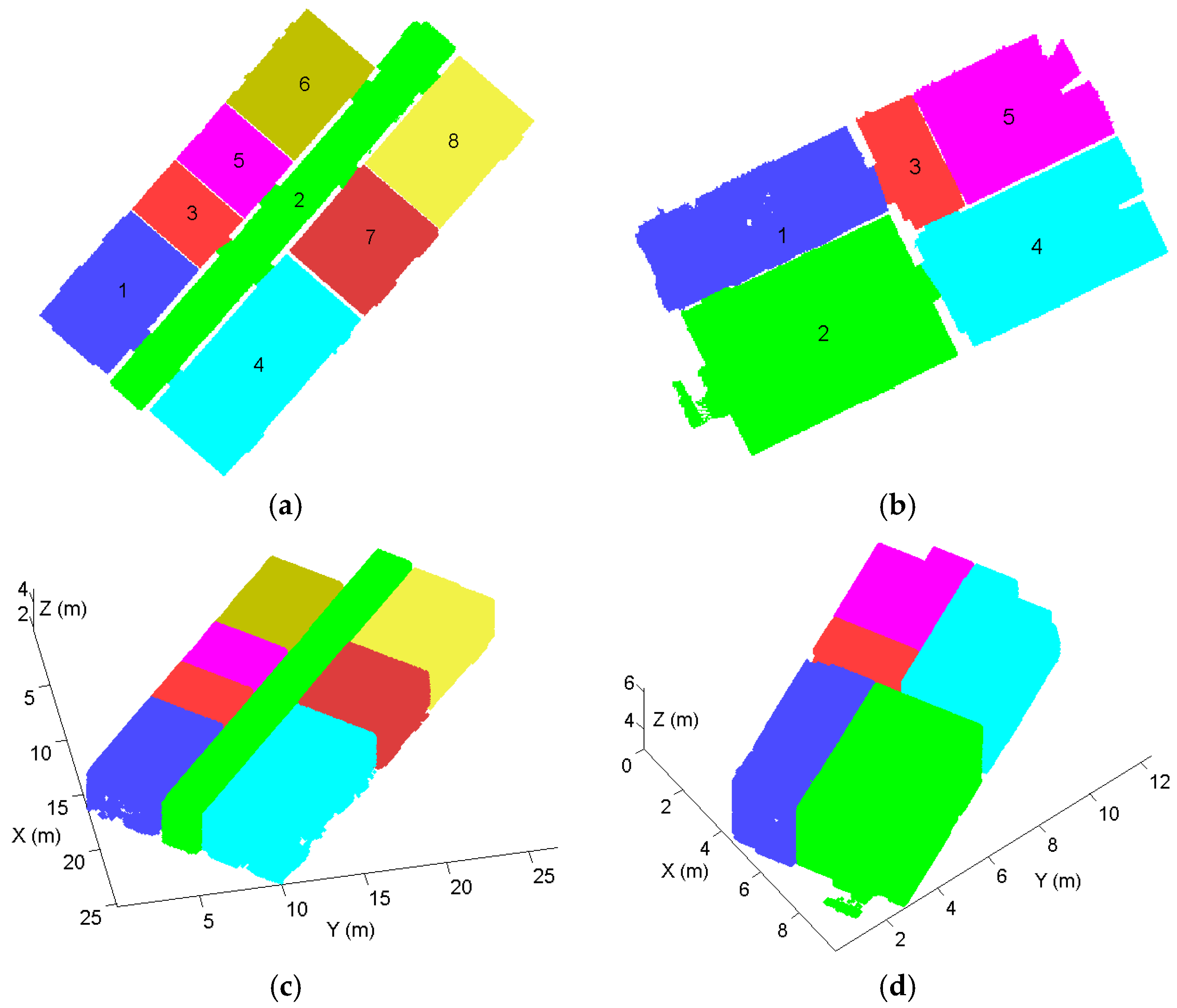
Figure 14.
Original point cloud of second real-world data set: (a) entire point cloud in plan view; and (b) noisy points between two wall surfaces.
Figure 14.
Original point cloud of second real-world data set: (a) entire point cloud in plan view; and (b) noisy points between two wall surfaces.

Figure 15.
Segmentation results for publicly available point-cloud data sets: (a,c,e,g) input point clouds; and (b,d,f,h) resultant segment maps.
Figure 15.
Segmentation results for publicly available point-cloud data sets: (a,c,e,g) input point clouds; and (b,d,f,h) resultant segment maps.


Figure 16.
Segmentation results for synthetic data sets: (a,c,e,g,i) input binary maps; and (b,d,f,h,j) resultant segment maps.
Figure 16.
Segmentation results for synthetic data sets: (a,c,e,g,i) input binary maps; and (b,d,f,h,j) resultant segment maps.

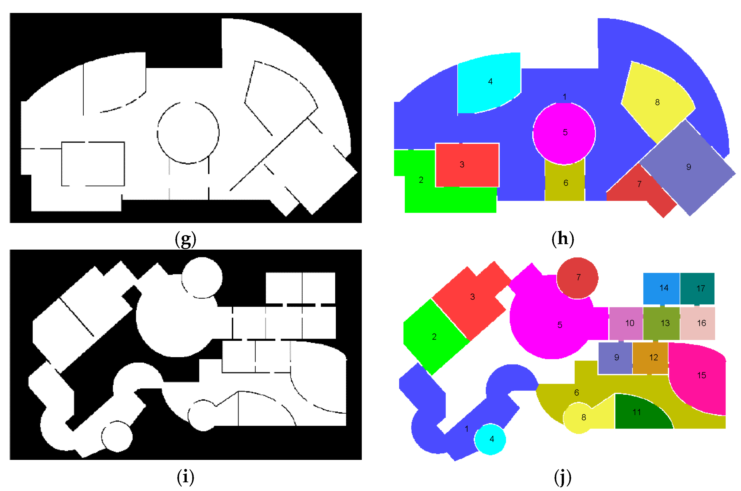
Figure 17.
Comparison of room segmentation approaches with non-furnished data sets: (a) ground truth by manual segmentation; (b) morphological segmentation; (c) distance transform-based segmentation; (d) Voronoi graph-based segmentation; (e) feature-based segmentation; (f) Voronoi random field segmentation; and (g) our room segmentation.

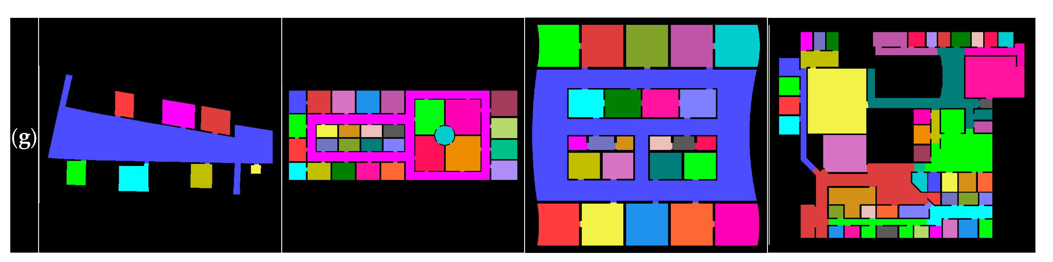
Figure 18.
Comparison of room segmentation approaches with furnished data sets: (a) ground truth by manual segmentation; (b) morphological segmentation; (c) distance transform-based segmentation; (d) Voronoi graph-based segmentation; (e) feature-based segmentation; (f) Voronoi random field segmentation; and (g) our room segmentation.

Table 1.
Summary of room segmentation methods.
| Properties | Domain | Input Data | Main Assumptions or Limitations | Supplementary Data | References | |
|---|---|---|---|---|---|---|
| Methods | ||||||
| Morphological | Robotics | Grid map | Narrow passages/2D data only | - | Fabrizi et al. [22] | |
| Distance transform | Robotics | Grid map | Narrow passages/2D data only | Virtual markers | Diosi et al. [23] | |
| Voronoi graph | Robotics | Grid map | Narrow passages/2D data only | - | Wurm et al. [20] | |
| Feature based | Robotics | Grid map | Resemblance between data/2D data only | Labeled map | Mozos et al. [33] | |
| Voronoi random | Robotics | Grid map | Narrow passages/2D data only | Labeled map | Friedman et al. [34] | |
| Probabilistic model | AEC | Point cloud | Planar walls | Initial labeling | Ochmann et al. [30] | |
| Iterative binary subdivision | AEC | Point cloud | Planar walls | Scanner locations | Mura et al. [15] | |
| Graph clustering | AEC | Point cloud | Vertical walls/Mobile data only | Scanner path | Turner [17] | |
| Height constraint | AEC | Point cloud | Vertical walls/No link at certain level | - | Macher et al. [18] | |
| K-medoids | AEC | RGBD images | Narrow passages/Manhattan world/Planar walls | - | Ikehata et al. [31] | |
| Proposed Approach | Robotics/AEC | Grid map/Point cloud | Narrow passages/Vertical walls | - | - | |
Table 2.
Parameter selections for two real-world data sets (unit: meters).
| Process Phase | Parameter (s) | Data 1 | Data 2 | Remark |
|---|---|---|---|---|
| Height estimation | Interval | 0.10 | 0.10 | User-specified |
| Rasterization | Pixel size | 0.05 | 0.03 | User-specified |
| Noise filtering | Noise-filtering offset | 0.50 | 0.40 | User-specified |
| Initial segmentation | Detection window size for finding initial segments | 1.55 | 0.99 | User-specified |
| Opening closure | Detection window size for finding surrounding walls | 3.10 | 1.98 | Automatic |
| Detection window size for pruning small branches | 1.55 | 0.99 | Automatic |
Table 3.
Summary of experiments with four publicly available point-cloud data sets.
| Data No. | Data Size (million points) | Pixel Size (meters) | Detection Window Size (meters) | Processing Time (sec) |
|---|---|---|---|---|
| 1 | 37.69 | 0.15 | 4.65 | 25.93 |
| 2 | 40.71 | 0.20 | 4.60 | 26.74 |
| 3 | 33.93 | 0.10 | 1.90 | 23.57 |
| 4 | 25.17 | 0.05 | 1.85 | 52.67 |
Table 4.
Test specifications for synthetic data sets.
| Data No. | Architectural Shape | No. of Room (segment/true) | Map Size (pixels) | Detection Window Size (meters) | Processing Time (sec) |
|---|---|---|---|---|---|
| 1 | Linear | 28/28 | 421 by 704 | 1.05 | 46.62 |
| 2 | Linear | 14/14 | 359 by 606 | 1.05 | 7.98 |
| 3 | Linear | 16/14 | 359 by 606 | 1.05 | 10.75 |
| 4 | Nonlinear | 9/9 | 359 by 606 | 1.55 | 27.69 |
| 5 | Nonlinear | 17/17 | 359 by 606 | 1.05 | 8.66 |
Table 5.
Evaluation metrics (mean ± standard deviation) as calculated over 20 publicly available data sets without and with furniture. The first and the second best results are highlighted in bold type.
Table 5.
Evaluation metrics (mean ± standard deviation) as calculated over 20 publicly available data sets without and with furniture. The first and the second best results are highlighted in bold type.
| Data Type | Non-Furnished | Furnished | |||||
|---|---|---|---|---|---|---|---|
| Properties | Correctness (%) | Completeness (%) | Absolute Deviation | Correctness (%) | Completeness (%) | Absolute Deviation | |
| Methods | |||||||
| Morphological | 81.9 ± 13.0 | 81.7 ± 13.5 | 5.2 | 78.3 ± 16.3 | 56.8 ± 15.0 | 6.1 | |
| Distance transform | 83.2 ± 14.5 | 82.1 ± 15.1 | 3.5 | 76.5 ± 17.6 | 51.4 ± 15.7 | 11.8 | |
| Voronoi graph | 95.0± 6.1 | 80.7 ± 7.6 | 10.1 | 94.0 ± 6.7 | 68.6 ± 8.3 | 11.7 | |
| Feature based | 78.0 ± 8.4 | 72.9 ± 10.7 | 4.7 | 79.8 ± 16.0 | 60.0 ± 15.3 | 8.5 | |
| Voronoi random | 90.0 ± 8.4 | 88.2 ± 10.0 | 2.9 | 81.0 ± 14.4 | 64.6 ± 14.6 | 5.4 | |
| Average | 85.6 ± 12.0 | 81.1 ± 12.5 | 5.3 | 81.9 ± 15.7 | 60.3 ± 14.7 | 8.7 | |
| Proposed | 89.6 ± 9.8 | 91.7 ± 9.0 | 2.5 | 84.8 ± 13.9 | 67.8 ± 14.5 | 8.2 | |
© 2017 by the authors. Licensee MDPI, Basel, Switzerland. This article is an open access article distributed under the terms and conditions of the Creative Commons Attribution (CC BY) license (http://creativecommons.org/licenses/by/4.0/).
Share and Cite
MDPI and ACS Style
Jung, J.; Stachniss, C.; Kim, C. Automatic Room Segmentation of 3D Laser Data Using Morphological Processing. ISPRS Int. J. Geo-Inf. 2017, 6, 206. https://doi.org/10.3390/ijgi6070206
AMA Style
Jung J, Stachniss C, Kim C. Automatic Room Segmentation of 3D Laser Data Using Morphological Processing. ISPRS International Journal of Geo-Information. 2017; 6(7):206. https://doi.org/10.3390/ijgi6070206
Chicago/Turabian StyleJung, Jaehoon, Cyrill Stachniss, and Changjae Kim. 2017. "Automatic Room Segmentation of 3D Laser Data Using Morphological Processing" ISPRS International Journal of Geo-Information 6, no. 7: 206. https://doi.org/10.3390/ijgi6070206
Note that from the first issue of 2016, this journal uses article numbers instead of page numbers. See further details here.