A Matrix-Based Structure for Vario-Scale Vector Representation over a Wide Range of Map Scales: The Case of River Network Data

Abstract

The representation of vector data at variable scales has been widely applied in geographic information systems and map-based services. When the scale changes across a wide range, a complex generalization that involves multiple operations is required to transform the data. To present such complex generalization, we proposed a matrix model to combine different generalization operations into an integration. This study was carried on a set of river network data, where two operations, i.e., network pruning accompanied with river simplification, were hierarchically constructed as the rows and columns of a matrix. The correspondence between generalization operations and scale, and the scale linkage of multiple operations were also explicitly defined. In addition, we developed a vario-scale data structure to store the generalized river network data based on the proposed matrix. The matrix model was validated and assessed by a comparison with traditional methods that conduct generalization operations in sequence. It was shown that the matrix model enabled complex generalization with good generalization quality. Taking advantage of the corresponding vario-scale data structure, the river network data could be obtained at any arbitrary scale, and the vario-scale representation was achieved across a wide scale range.

1. Introduction

The representation of vector data at variable scales has been widely applied in geographic information systems and map-based services, e.g., OpenStreetMap, Google Maps and Crowdsourcing maps [1]. With the advances in Geoweb [2], vario-scale representation is not only utilized to present data at any appropriate level of detail (LoD), but is also required to facilitate data transmission and knowledge discovery using its data abstraction technologies [3,4]. Given varied objectives and application domains, such as displaying a topographical map on both a wall screen and smart phone, tailoring a set of volunteered geographic information data (e.g., vehicle trajectories and geotagged place names) to fit a few user-defined mashups [5], spatial representation should be adaptable in variable LoDs (levels of detail) over a wide range of map scales.

To achieve a vario-scale representation of spatial data, cartographers apply map generalization to generate coarse LoDs from a given detailed data set [6,7,8]. A large number of generalization operations can be used: elimination is used to remove one or more geographic features to reduce the content for display; simplification removes points from a line or polygon boundary to reduce unwanted small details; merger combines connected or adjacent features into a single feature without changing dimension; and so on [9]. As for network generalization, elimination also refers to pruning, selection, or thinning, which concern topological maintenance and data model integrity [10,11,12,13]. Note that these generalization operations also transform data at different aspects. Some may affect groups of map objects or individual map objects (e.g., elimination vs. simplification), while others may lead to changes in topology or geometry (e.g., merger vs. simplification). When the map scale changes across a wide range, generalization often requires a complex process that adopts multiple operations to ensure satisfactory generalized results that meet the application requirements.

Ideally, the generalization process should be holistic, and fundamentally depends on the scales and feature class involved (e.g., rivers, buildings, or points of interest). However, as one generalization operation only addresses one specific generalization issue, the complex process has to be broken down into a set of sub-processes, and relevant operations are then conducted in series to output an abstracted result [14]. Two major problems currently exist. First, only a few studies have been concerned with how to properly organize different generalization operations into a rational workflow. According to Cecconi [15], the generalization operations are non-homogeneous within the range of map scale. Though selection (or elimination by Stanishlawski) and simplification act as two common operations through the complete scale range, other operations may take place at different scale ranges. Some studies have tried to orchestrate the logic sequence of generalization operations for particular scales [16,17,18], but it was argued that performing the operations in different orders would generate completely different results [19]. Thus, a model that combines multiple operations for a range of scale is still missing. Second, though numerous algorithms have been developed for various generalization operations [8,20,21,22,23], the tolerance parameters for scales change were determined separately as the linkage between the tolerance parameters of multiple operations were not considered during the generalization. Thus, the issue of vario-scale representation involving multiple generalization operations still requires future study.

In this paper, we present an integrated model to combine different generalization operations for vario-scale representation. In our previous work [11], a matrix diagram was presented to describe the progressive selection and simplification of a hydrographic network. As the involved operations were performed separately (i.e., the network was pruned before the flowlines were simplified), reasonable generalization results could not be confirmed (as shown in Figure 1). A number of points, which should have been removed from the flowlines, were kept to preserve the topological relationships between adjacent branches. This study extends our previous work in three areas: (1) developing an integrated matrix to organize hydrographic LoDs raised by different operations, i.e., selection (network pruning) and simplification, as a hybrid hierarchy; (2) defining the scale correspondences of two involved operations; and (3) establishing a vario-scale structure to assemble the data based on the integrated matrix to provide vario-scale representation at any scale required.

This study was conducted on a set of river network data extracted from the Multiple Representation Database (MRDB) produced by the China National Geographic Information Institute. We assumed that the river network consisted of linear elements, and the polygonal river channels and other area elements were substituted by their linear counterparts. The complex generalization was confined to the combination of selection operations (i.e., pruning the river network) and the simplification operation (i.e., simplifying the rivers) concerned. The remainder of this paper is organized as follows: Section 2 reviews the relevant work. In Section 3, first, our generalization methods including network pruning and river simplification are presented to define the sequence of LoDs for scales. Then, a hybrid matrix is developed to integrate the generalized results. In Section 4, the scale correspondence of generalization operations in the matrix is investigated. Section 5 establishes a vario-scale data structure based on the proposed matrix, and Section 6 assesses the matrix model through a comparison with traditional solutions referring to sequence generalization through an empirical study. Finally, Section 7 concludes the paper and provides an outlook for future work.

2. Relevant Work

Vario-scale representation refers to the situation where the LoD at any arbitrary map scale can be obtained by an automatic generalization process [24]. It is quite different to multi-scale representation, which provides LoDs representation for a fixed number of scales. Furthermore, vario-scale representation supports continuous and topologically consistent transformation without abrupt changes [25]. With respect to vario-scale representation of river networks, related research involves at least three aspects: continuous generalization, vario-scale data structure, and hydrographic generalization.

2.1. Continous Generalization

Continuous generalization aims to produce maps that adapt the generalization degree to any scale in a continuous way [26,27,28]. When LoD representation changes from one scale to another, intermediated states can be defined to provide a smooth transfer. To achieve continuous generalization, efforts were made based on interpolation technologies, which are known as morphing in computer graphics and computational geometry [28,29]. These efforts usually include two phases: to find the corresponding data at two scales; and to specify the trajectory that connects the pairs of corresponding data. Due to the lack of algorithms for spatial correspondence and trajectory specification without spatial conflicts, morphing-based generalization still remains a challenge. Some scientists have suggested another option where the incremental generalization generates a more detailed representation with small incremental changes. In addition, algorithms have been mainly reported in the literature for line simplification [30]; building ground plans displacement [27]; and land use area aggregation [31]. We categorized our study into the incremental generalization.

2.2. Vario-Scale Data Structure

A data structure that stores data of variable scale in terms of vario-scale data structure enables a promising application to deliver LoDs with continuous transformation [25,32,33,34,35]. This has been proposed to overcome the drawback of multi-scale data structures, which support only a limited number of scale intervals with data redundancy [15,25]. A few vario-scale models have been successfully carried out, including the Binary Line Generalization tree (BLG tree) [36], Reactive tree [37], topological Generalized Area Partitioning (tGAP) structure [33], and Simple Operations (SOs) vocabulary [27]. Most of these focus on a single generalization process, such as simplifying, merger, and displacement, and are used to provide progressive data transfer with less data redundancy. Additionally, existing vario-scale structures are still rare.

2.3. Hydrographic Generalization

Hydrographic generalization produces LoDs representations for hydrographic feature (i.e., rivers, stream, and lakes). It is one of the basic topics in map generalization. Over the last few decades, plenty of generalization operations have been applied to derive coarse hydrographic data such as simplification to remove small geometric variations in the flowline or lake boundary; selection for pruning (i.e., thinning) the river network; aggregation to combine an array of closed ponds; and collapse to replace the narrows rivers with a linear counterpart.

Increased research in this area has indicated that complex generalization (referring to multiple operations) should be applied to generate reasonable hydrographic LoDs [11,15,17,19,38,39]. For instance, Buttenfield et al. [17] specially tailored generalization operations and their processing sequences based on the physiographic diversity. Considering the river network, the pruning (i.e., selection) operation had a higher priority. Additional operations which either removed or modified details from individual rivers were then implemented post-pruning. Other research have also suggested that network pruning and river simplification should act together during the overall process of hydrographic generalization [11,15,38].

To present the complex generalization, we proposed an integrated matrix by modeling the generalization process (consisting of network pruning and river simplifying) as a hybrid. This then carried out the corresponding generalization algorithms in combination. Beyond that, we developed a vario-scale data structure to store the generalized river network data based on the matrix model. This vario-scale structure enabled us to generate river network data for an arbitrary scale, and supported vario-scale representation across a wide scale range.

3. Matrix Model for Vario-Scale Representation

The basic idea of the model is to present multiple generalization operations as different dimensions of a matrix, so that the complex generalization process can be achieved by sliding the matrix. For the river network, we hierarchically constructed the network pruning and river simplification as the rows and columns of the matrix. The procedure contained the following steps: first, defining the hierarchical LoDs of the river network and individual rivers, before combining them into a hybrid structure.

In the following sections, the term river refers to a complete flow path that may consist of one or a series of segments in the river network. Node means the point by which two rivers are connected. The term segment refers to the channel between to two consecutive nodes.

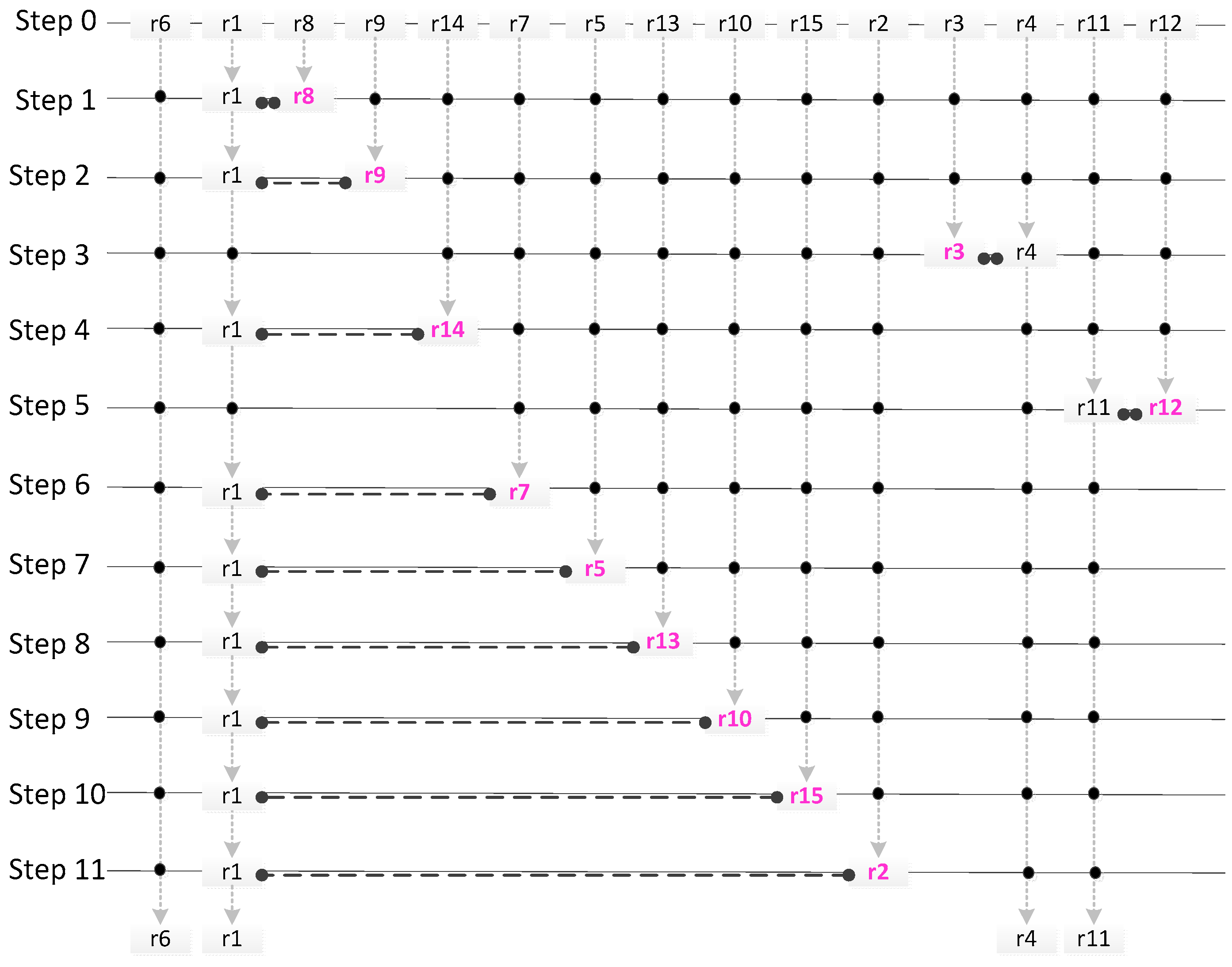
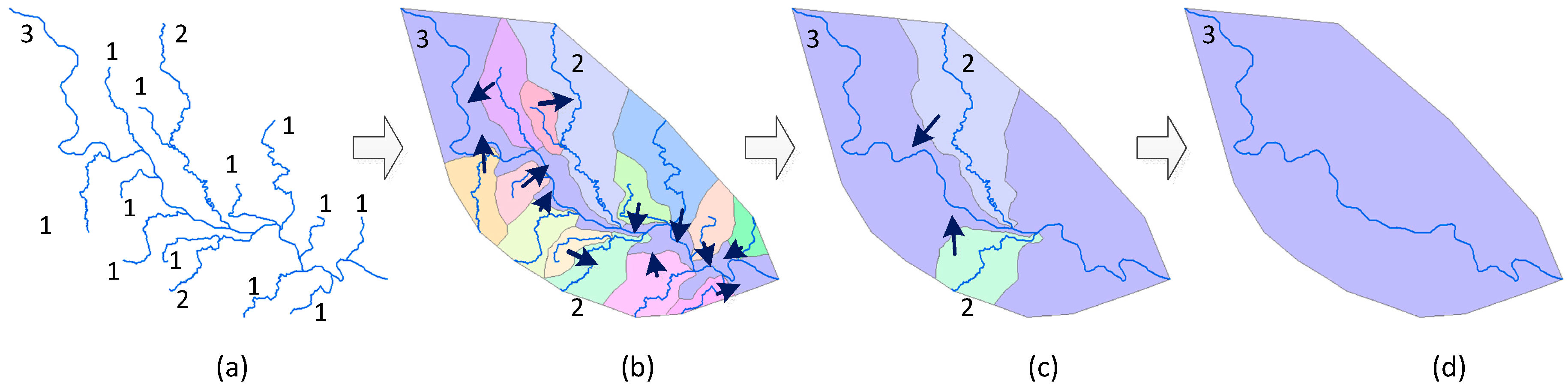
3.1. Hierarchical Construction for Network Pruning

Network pruning, or eliminating rivers from the river network while still maintaining the correct topology, is a common operation in hydrographic generalization. A number of pruning methods have been proposed based on various hydrographic factors, such as river length, Horton code, watershed partition, and upstream drainage area (UDA) [40,41,42,43]. The key consideration is to measure the importance of rivers so that rivers of higher importance are preserved, and those of low importance eliminated.

In this study, the importance of rivers was measured considering watershed partition [43], associated with the length, hydrographic topology, and feature class of the rivers. The procedure of watershed partition is shown in Figure 2. First, rivers were labelled with the Horton code [44]; then, the watershed area of each river was created using the linear constrained Voronoi diagram [45]. Next, the watershed area corresponding to the lowest-order label merged iteratively with the watershed area that had a higher order label. Based on the watershed partition, the importance value of each river in a network can be specified as follows:

$$Imp\left(i\right)=\omega \left(i\right) \times Length\left(i\right) \times Area\left(i\right),$$

where the importance value of river $i$ is presented as $Imp\left(i\right)$; the length of river $i$ is presented as $Length\left(i\right)$; and the area of the corresponding watershed containing all its sub-watersheds was presented as $Area\left(i\right)$. Furthermore, we introduced a class-dependent weight factor represented as $\omega \left(i\right)$. The value of $\omega \left(i\right)$ varied due to the hydrographic pattern of river network. For instance, a river in a high density area had a smaller value than one in a low density area. The calculation of $\omega \left(i\right)$ was beyond the scope of this study, so to consider the distribution of the river network relatively evenly, we used a constant weight of 1 for all rivers.

Network pruning was carried out step-by-step by sorting the rivers into a descending order of importance; subsequently, the LoDs of the river network were derived in a progressive manner. Figure 3 illustrates the stepwise procedure. For each step, the least important river was eliminated from the network, which was not always the shortest, lowest order, or related to the smaller watershed area. The river segments adjacent to the eliminated river were merged. This procedure is presented as a linear hierarchy shown in Figure 4.

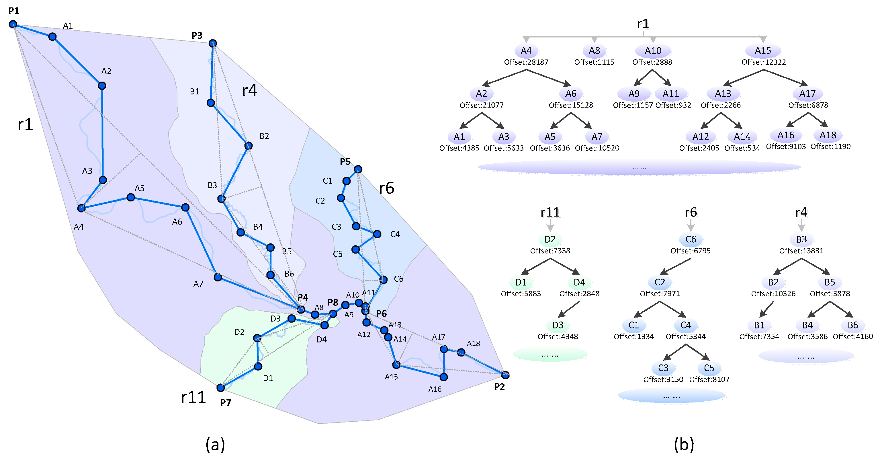
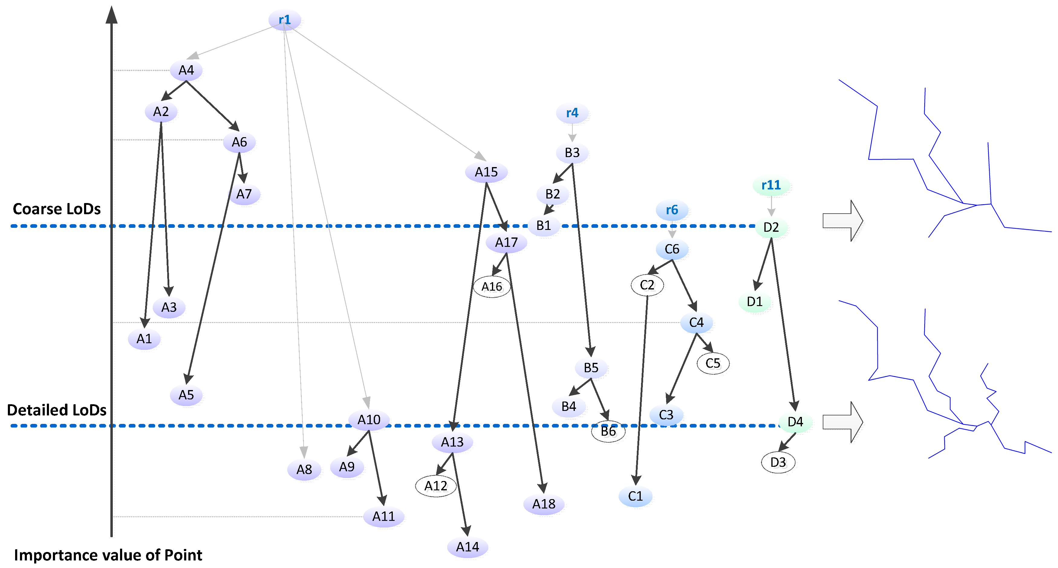
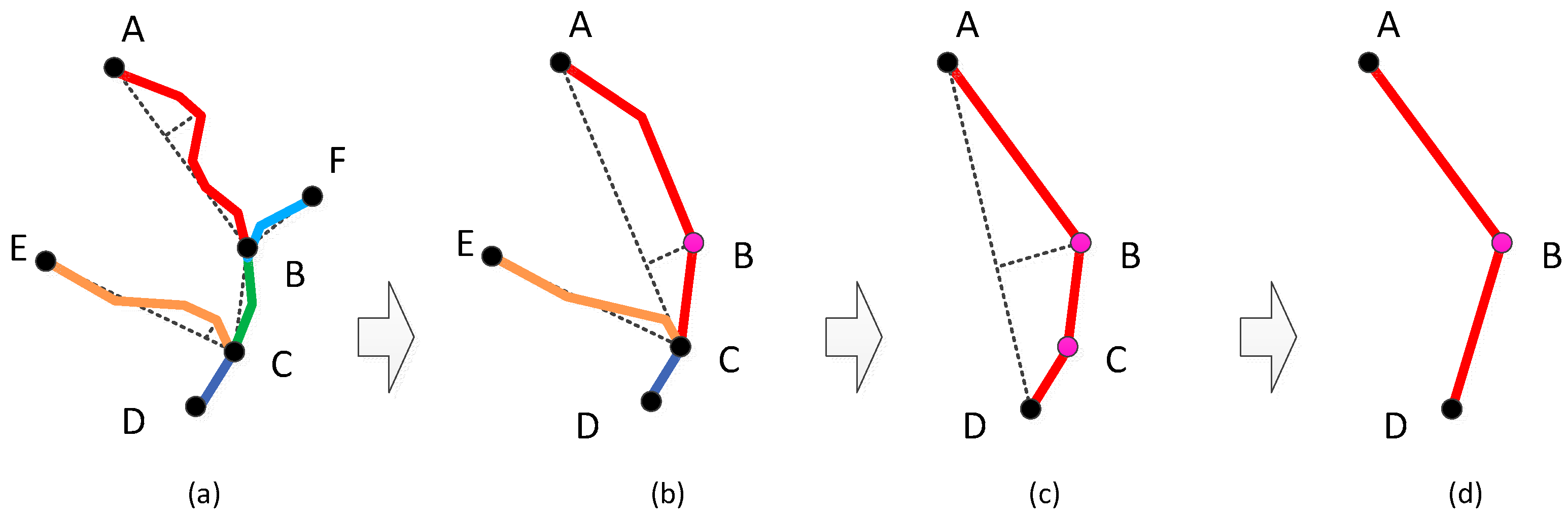
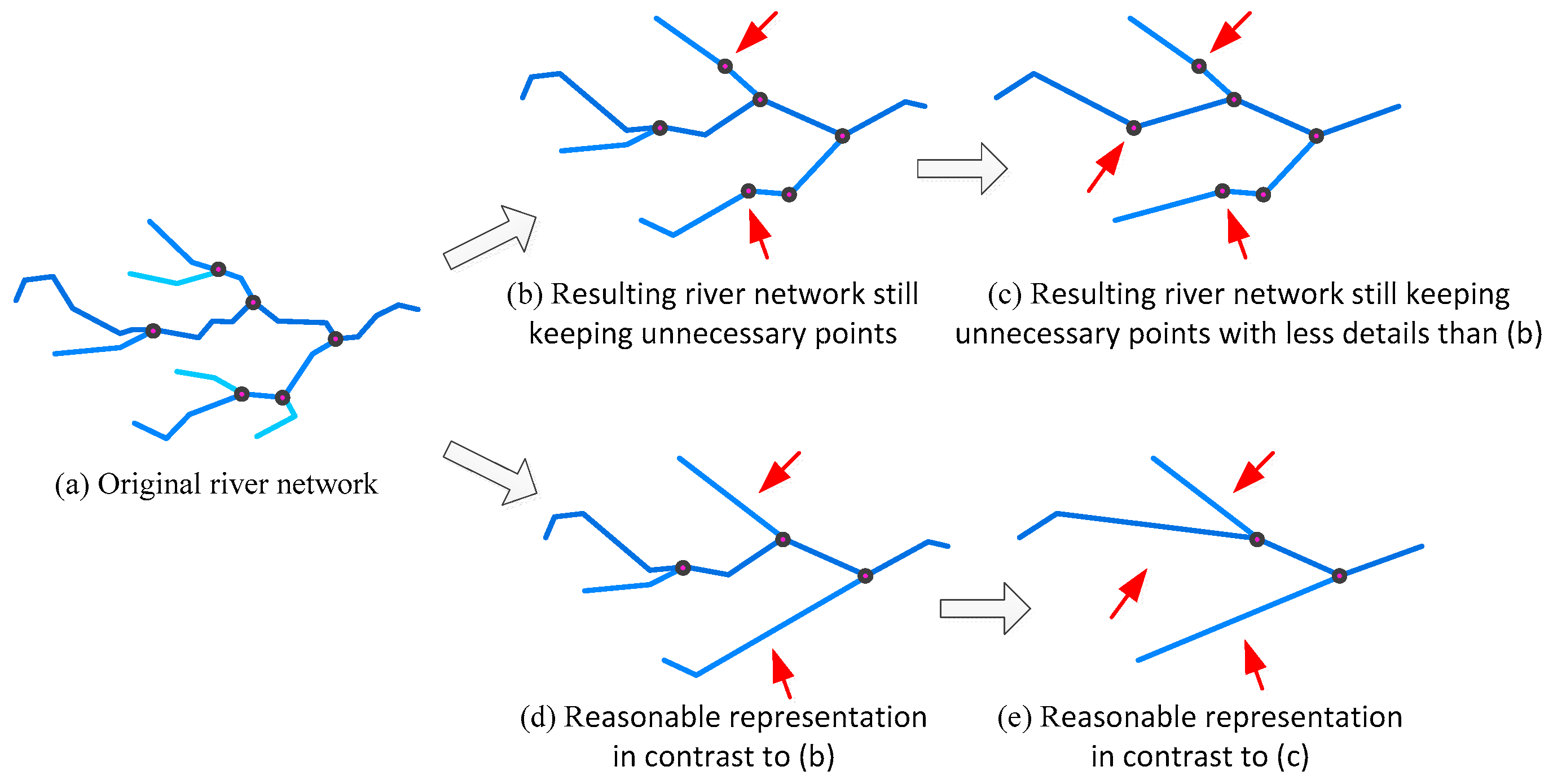
3.2. Hierarchical Construction for River Simplification

During network pruning, the preserved rivers were also appropriately simplified. Considerable simplification algorithms can be used [22,46,47]; it has been noted that the well-known Douglas–Puecker (DP) algorithm, which selects the critical or shape-describing points globally and iteratively, has the best performance out of the other algorithms in terms of data accuracy and reduction [46,48]. Therefore, we applied a modified Douglas–Peucker algorithm advanced by Meijers [49] for the simplification of grouping lines.

For a single river, the offset of points to the corresponding base line was calculated. Taking the river segment P1P4 in Figure 5 for instance, a straight line P1P4 was regarded as the base line, then the distance from point A4 to the base line was measured as the offset of point A4. Next, the intermediate point with the maximum offset was selected as the significant point and used to divide the river into two parts. The offset was also recorded as the importance value of the point. For rivers in group, the river with the highest priority in selection was simplified first, before the less important river was simplified using the more important river as the constraint. The topological relationship between the simplified river and the simplified and constrained river was checked during the simplification. In cases where a local conflict arose, points with the second or third maximum offset were selected instead of the maximum offset.

Due to the recursive nature of the DP algorithm, it was able to retrieve the shape-describing points from rivers to define a set of BLG trees hierarchically for LoDs representation (as shown in Figure 5). To maintain the correct adjacent relationship between rivers, we used the simplification operation on segments. Thus, the point hierarchy for an individual river may be constructed as a forest (i.e., several trees present the related river segment) rather than a single tree. Cutting off the point hierarchy using different tolerances provided generalized rivers at various LoDs (as shown in Figure 6).

Note that, in the point hierarchy, the offset distance of a parent point may be smaller than those of its child points. For instance, the offset distance of A13 and A12 was 2266 and 2405, respectively, in Figure 5, and it was not guaranteed that a higher level point had a larger offset than that of a lower level point. Therefore, we set the offset of the child point equal to its parent points. In Figure 6, the offset of A12 was changed to 2266, equal that of its parent point A13. In this way, the hierarchical structure was transformed into a linear storage structure by first adding the two end points of the river section, and then appending the remaining points in an offset-decreasing order, as shown in Figure 7. By selecting points from left to right in this linear structure, it was easy to reconstruct the river lines of different LoDs. The selected points were adjusted in correct sequence as in the original line.

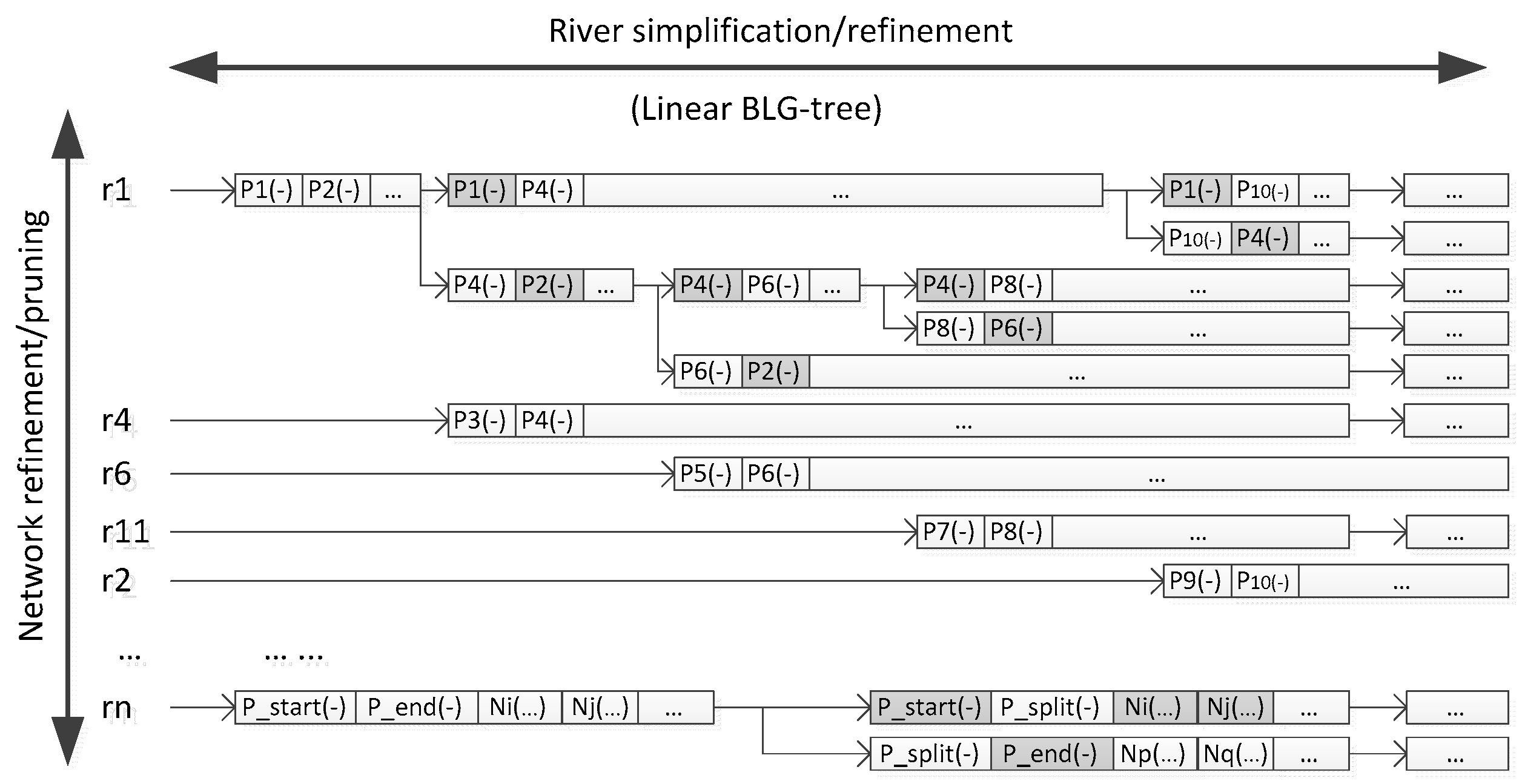
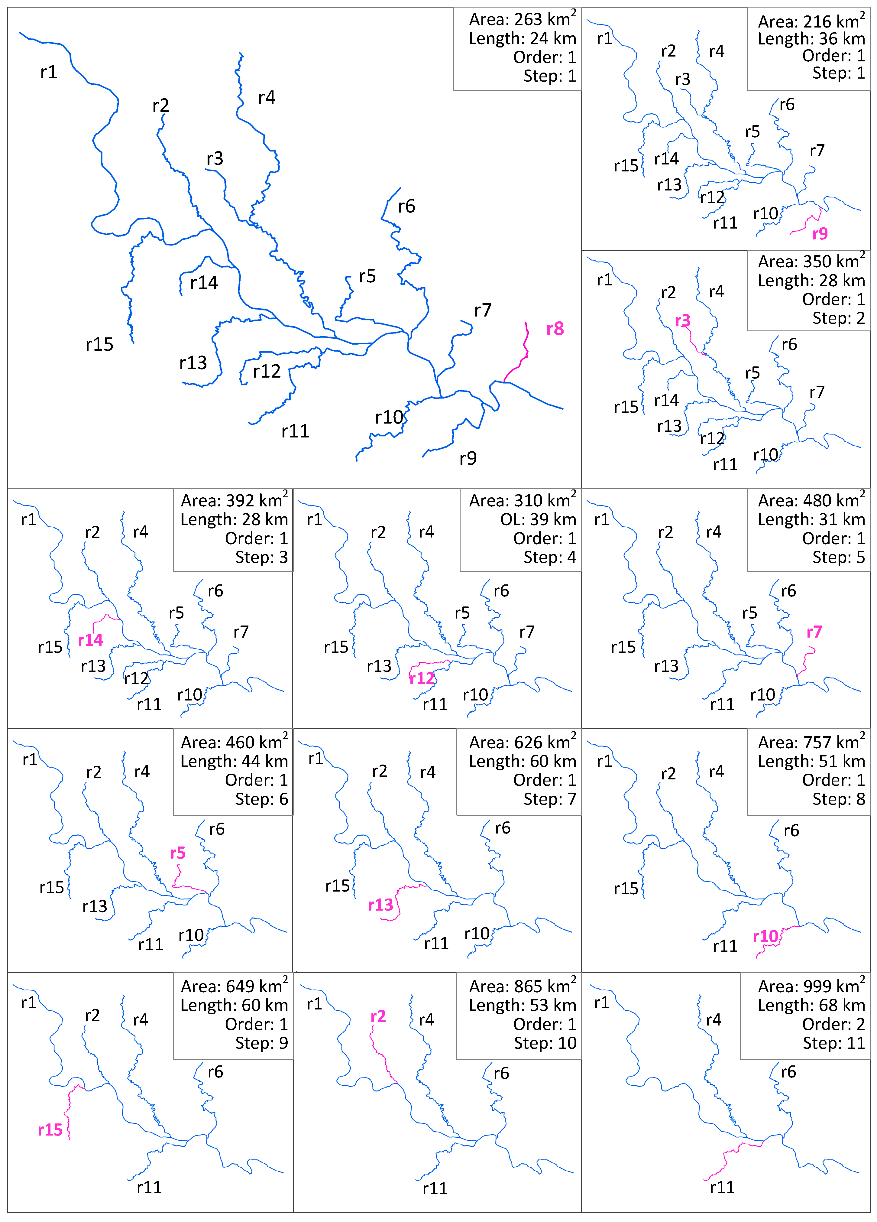
3.3. A Matrix Hybrid: Integration of Network Pruning and River Simplification

As both network pruning and river simplification were constructed in linear hierarchies of LoDs, it was easy to describe the complex process using a matrix diagram, where the rows represent river lines ordered by importance, and the columns the sorted points of a river [11]. The key was to integrate these LoDs into a comprehensive pattern.

Figure 8 demonstrates the complex generalization of a river network. When a river was eliminated, two adjacent segments were properly simplified, and merged as a new segment for the subsequent process. Such a merger arose as a turning point in river simplification. Furthermore, the corresponding simplification of merged segments were presented in one BLG tree instead of two separated trees, and some important points became less important after the merge, such as point C.

To present the transformation, we constructed a matrix structure following the conceptualization of the tGAP tree advanced by van Oosterom [33]. That is, for each merger (corresponding to the river pruning), the matrix column was reformed by creating a new BLG tree to represent the simplification process of the merged segment. A schematic representation of the matrix hybrid is illustrated in Figure 9.

Therefore, the matrix hybrid of a river network can be built as follows:

• Construct the linear hierarchy of the river network by sorting the rivers in descending order of importance.
• Select the least important river from the river hierarchy, simplify its shape and construct a corresponding linear BLG tree that refers to the LoDs representation. Identify the river as an eliminated river.
• Check the river hierarchy and search the parent river which is adjacent to the current eliminated river (e.g., r1 is the parent river of r11 in Figure 5), retrieve the related segments (e.g., segment P4P8 and P8P6 of r1), then construct their linear BLG trees.
• Merge the adjacent segments, construct a new tree for the newly merged segment and insert in front of the original two linear trees. The original linear BLG trees of those adjacent segments are clipped at the relevant LoDs of the eliminated river.
• Repeat steps 2–4 until no rivers are left in the river hierarchy.

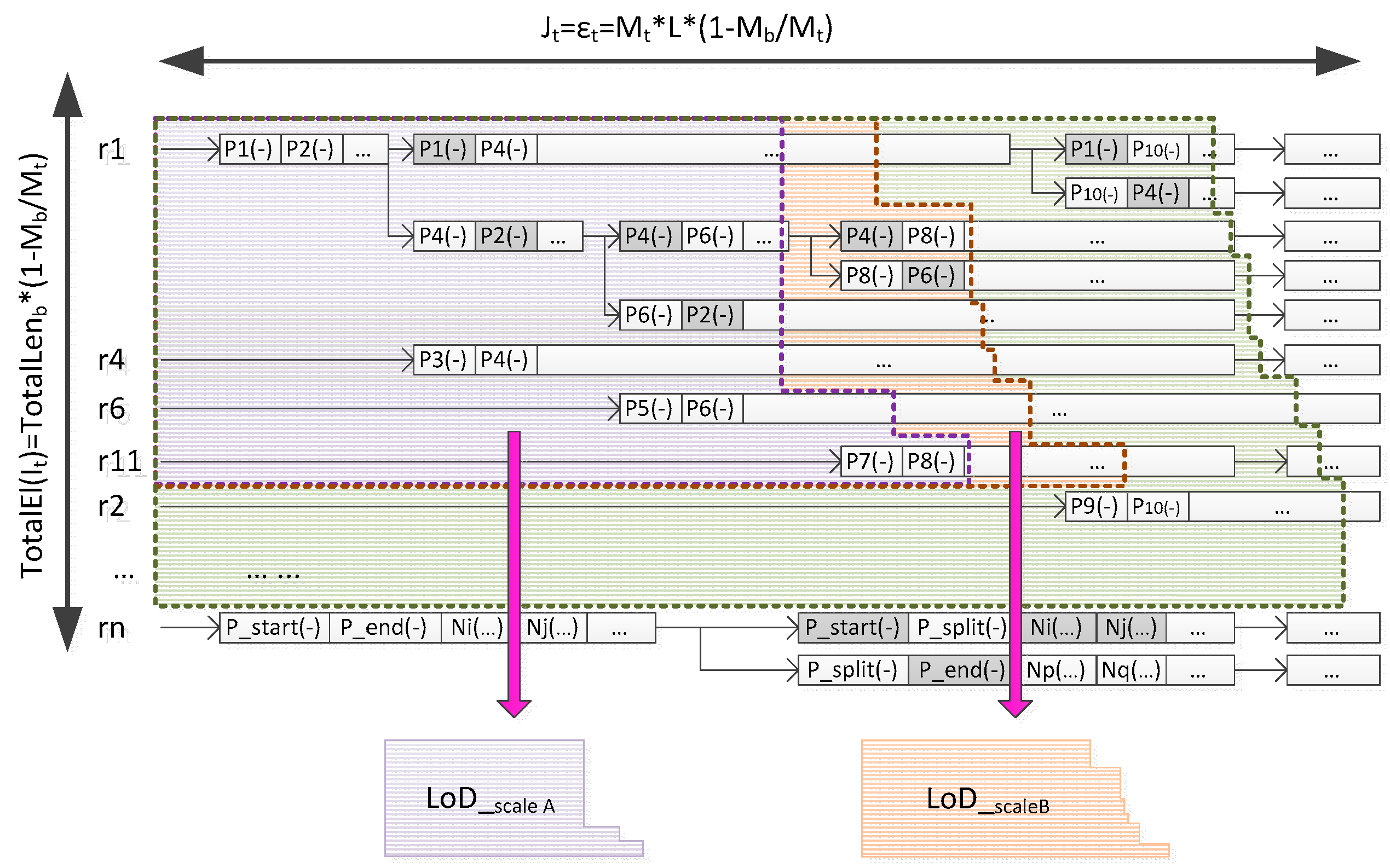
4. Scale Correspondence in the Matrix

Scale correspondence refers to the relationship between the LoDs and scale, as well as the scale linkage among different LoDs. In our study, we established scale correspondence for the proposed matrix through connecting the row and column that represented the sequence of LoDs to map scale, whilst associating each row with a column by the scale. Utilizing the corresponding scale, it was able to retrieve any LoDs by scanning the rows and columns of the matrix.

4.1. Three Scale Correspondences

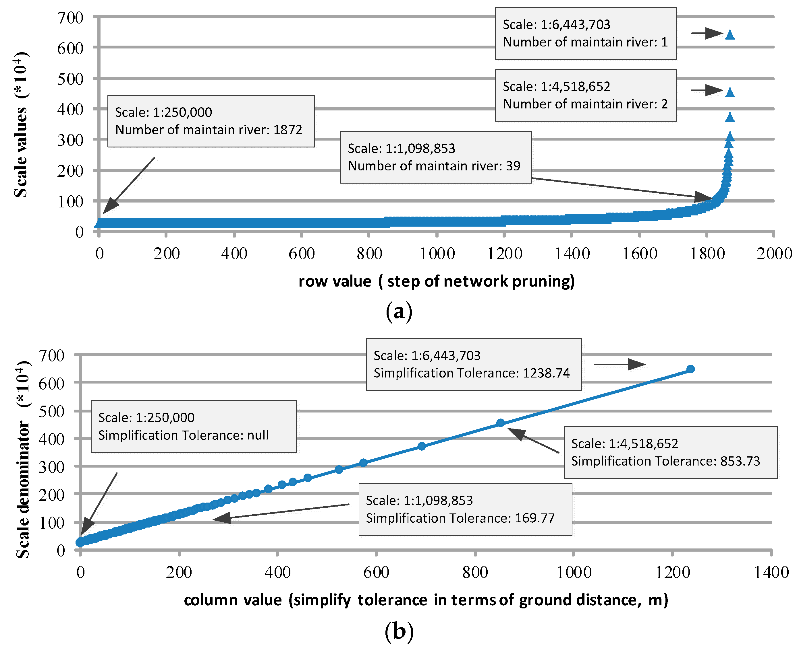
4.1.1. Scale Correspondence of the Row

During the network pruning, the least important river was removed from the map in a stepwise manner. According to Töpfer’s Radical Law, which is widely applied, the ratio of river amount at two scales should be proportional to the ratio of map scales [20]. The calculation can also be modified by replacing the river amount with the summed length of rivers [10,17]. Given the continuity of rivers and the topologic constraint of network, we presented the relationship between the statistic of river network and the map scale as follows:

$$\frac{TotalLe{n}_t}{TotalLe{n}_b}=\frac{M_b}{M_t}$$

(1)

where $M_b$ represents the scale dominator of the source (base) map, and $M_t$ is that of the target map; the symbols $TotalLe{n}_b$ and $TotalLe{n}_t$ represent the summed length of rivers at corresponding scales.

Then, the relation between scale and row (i.e., the step of pruning) can be expressed by:

$$TotalEL\left(I_t\right)=TotalLe{n}_b\times \left(1-\frac{M_b}{M_t}\right)$$

(2)

Here, the symbol $I_t$ means row and $TotalEL\left(I_t\right)$ means the summed length of rivers that have been eliminated. The calculation of $TotalEL\left(I_t\right)$ is approximate, as the entire river will be eliminated at each pruning step.

4.1.2. Scale Correspondence of the Column

As for river simplification, the retrieval of the shape-describe points was conducted using a simplification tolerance $\mathsf{\epsilon }$ which refers to the smallest visible offset distance. Using the symbol $L$ to represent the minimum length that can be visually identified on a map (in terms of map distance) [50,51], we presented the column $J_t$ based on the calculation of simplify tolerance ${\epsilon }_t$ as:

$$J_t={\epsilon }_t=M_t\times L\times \left(1-\frac{M_b}{M_t}\right)$$

(3)

4.1.3. Scale Linkage between Row and Column

The scale linkage between row and column was established on the basis of topology change that happened during the generalization of the river network. For each step that a river was removed whilst the adjacent segments were merged, the scale relation between row and column can be denoted as:

$$M_t\left(I\right)=M_t\left(J\right)$$

(4)

Here, $M_t\left(I\right)$ is the scale dominator corresponding to row and $M_t\left(J\right)$ is the scale dominator corresponding to the column. Thus, the linkage between row and column can be expressed by:

$$J_t=\frac{TotalEL\left(I_t\right)\times M_t\times L}{TotalLe{n}_b}$$

(5)

As map scale is used as the measure base of both row and column, the vario-scale representation can be consequently derived by top-down scanning on rows and left-right scanning on columns in the matrix until the required scale is reached. The results of the matrix scanning are illustrated in Figure 10. The selective data elements in the matrix behaved as an expanding area from the top left to bottom right corner.

4.2. Parameter Determination

Among all the above-mentioned parameters, the parameter ${\mathrm{M}}_{\mathrm{b}}$, ${\mathrm{M}}_{\mathrm{t}}$ and $TotalLe{n}_b$ are always known, but the L needs to be considered further. Several researchers have carried out this investigation; for instance, Muller [52] suggested 0.4 mm as an appropriate value L. Chen et al. [53] recommended a value of 10 mm. Li and Zhou [54] proposed that the parameter value should be in an appropriate range for different map series, e.g., from 0–25 mm.

There were two ways to determine the L value for the proposed matrix. One was to customize the smallest acceptable graphic distance based on the map applications. The other as to calculate the similarity of the vario-scale results derived from the matrix and the corresponding benchmark.

According to the Amos’ similarity [55], the similarity of the river network at two scales can be measured as:

$$Similarity=\frac{{\sum }_i(A\cap B)}{\sum A+\sum B-{\sum }_i(A\cap B)}$$

(6)

where $\sum A$ is the summed length of the rivers in LoD derived from the vario-scale matrix; and $\sum B$ is the summed length of the rivers in the benchmark. The symbol ${\sum }_{\mathrm{i}}(\mathrm{A}\cap \mathrm{B})$ is the summed length of the rivers common to the LoD and benchmark. In our study, we selected the common rivers from the LoD and Benchmark by querying their attribute ID, for example ${\mathrm{R}}_{i\_A}$ and ${\mathrm{R}}_{i\_B}$, then the length of the shorter river (either from the LoD or Benchmark) was summed up as $\mathrm{A}\cap \mathrm{B}=\min \left(\mathrm{length}\left({\mathrm{R}}_{i\_A}\right),\mathrm{length}\left({\mathrm{R}}_{\mathrm{i}\_\mathrm{B}}\right)\right)$.

To determinate the appropriate value of L, an empirical study was carried out on the experimental river network data. The topological river network at 1:250,000 was used as original data to establish the matrix and the data at 1:500,000 and 1:1,000,000 were used as the benchmark for the similarity evaluation. The initial range of L was from 0.01–5 mm with 0.01 mm as an interval.

The relationship between parameter L and the similarity is presented in Figure 11. Theoretically, the peak similarity of the series comparison indicated the most appropriate value of parameter L. As shown in Figure 11, it was easy to determine a peak range of similarity in each case. The appropriate values of L were also determined. In the cases of 1:500,000 and 1:1,000,000, the appropriate L was approximately 0.2 mm. Therefore, we used it as the appropriate value of L for the current series of maps.

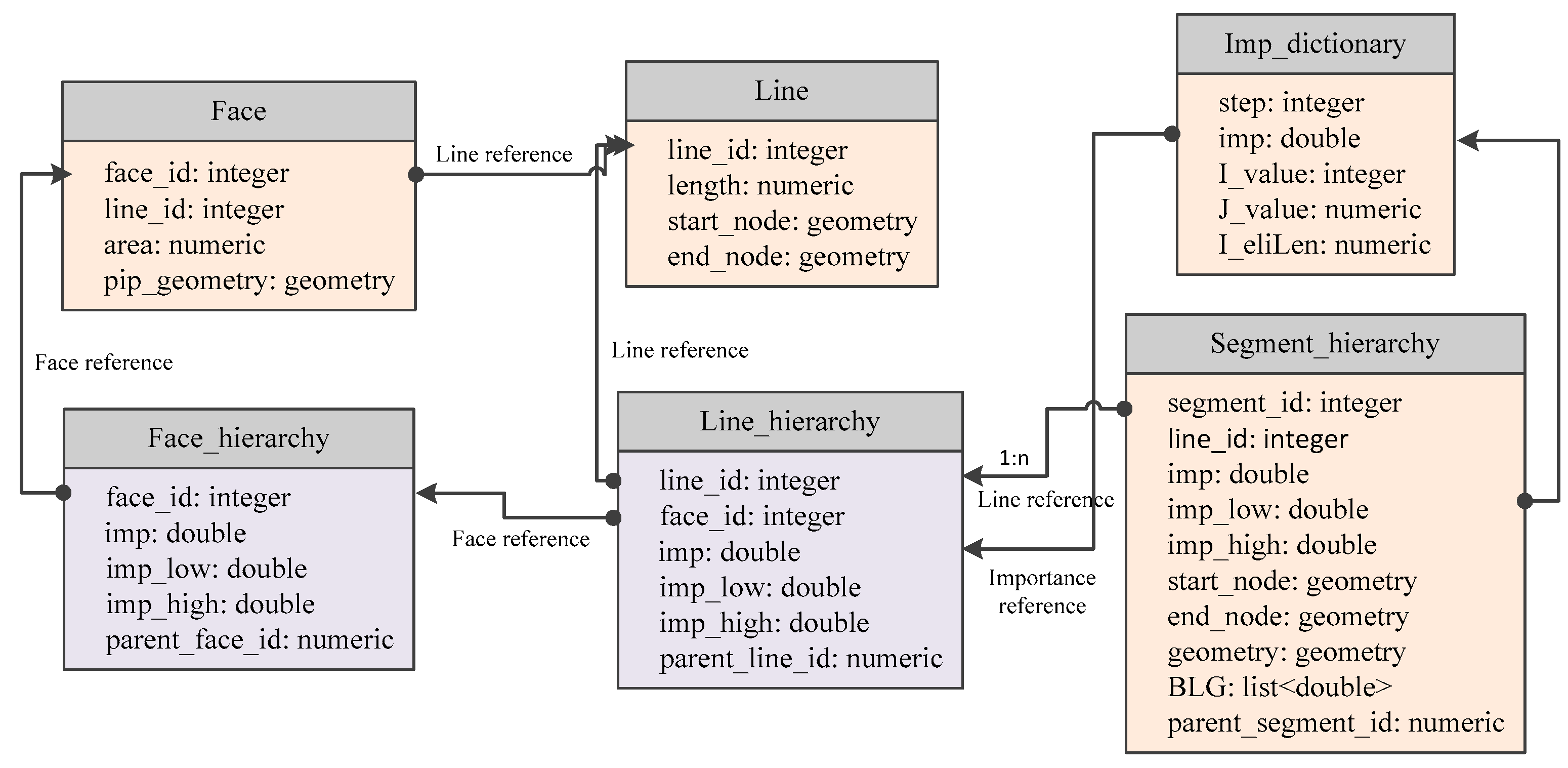
5. Vario-Scale Data Structure Based on the Matrix

In light of the integrated matrix proposed in Section 4, we implemented the physical storage of the complex generalization using a vario-scale data structure, which consists of several tables: Face, Line, Face_hierarchy, Line_hierarchy, Segment_hierarchy, and a lookup table Imp_dictionary. The table definitions and relationships are given in Figure 12. Some notes are as follows:

• Face refers to the watershed area represented in the polygon. Table Face records the area, and the length of the related river.
• Line refers to the river that is comprised of a few segments.
• Table Face_hierarchy records the importance values of the watershed area. The column imp records the importance value for each record, and the columns imp_low and imp_high indicate the importance range. Parent face refers to the watershed area which the current watershed area merges with.
• Table Line_hierarchy is joined with table Line and Face_hierarchy by line_id and face_id.
• Table Imp_dictionary stores the stepwise process of network pruning. The column imp records the importance value of eliminating rivers for each step. The I_value equals to step and is added for illustration purposes referring to the row of the matrix. The J_value is the simplified tolerance when a less important river is eliminated and two adjacent segments are merged. The I_eliLen means the summed length of all the removed rivers, i.e., $TotalEL\left(I_t\right)$ in Section 4.1.
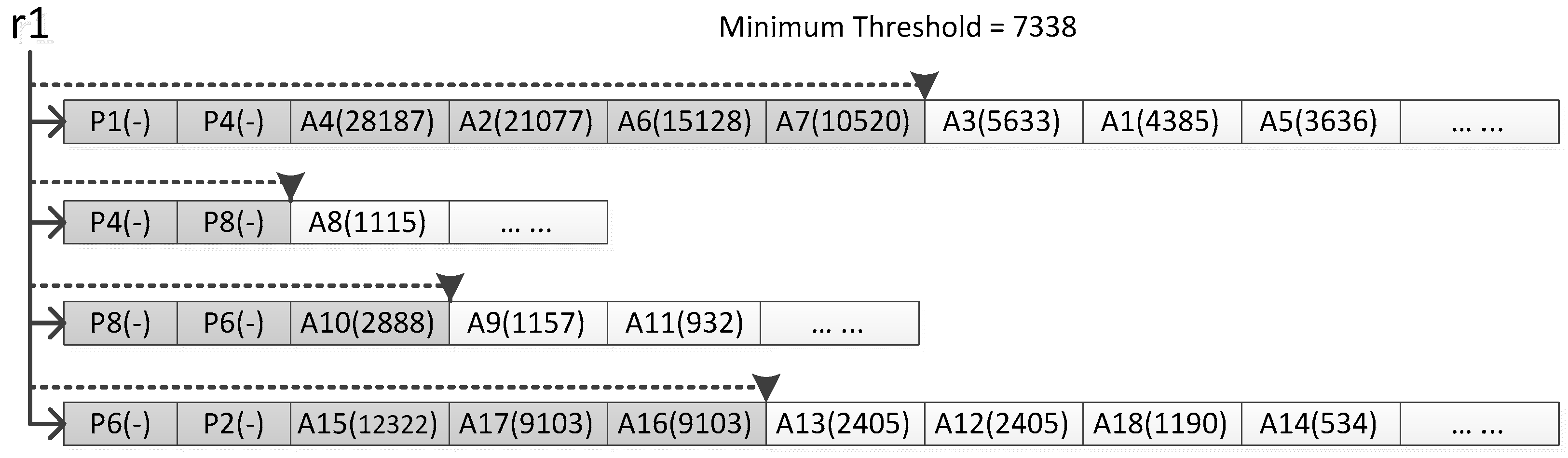
• Table Segment_hierarchy stores the process of segment simplification and mergers. A record refers to either an original river segment or a new segment merged from two adjacent segments. The BLG is a list of offset distance of the points in each segment. The parent_segment_id indicates the id of its next river segment going down the river.
• In the able Segment_hierarchy, the imp_low of segment equals the imp_high of eliminated river that causes the creation of the current segment. For an original river segment, the value of imp_low is 0. The imp_high of segment equals the imp_high of eliminated rivers, which lead the current segment to merge with another.

The vario-scale data structure does not explicitly store the LoDs representation of the river network. When a scale is given, the LoD representation will be derived dynamically via the following steps:

Step 1:

calculate the summed length of eliminated rivers $eliLen\_t$ for desired scale $m\_t$ by Equation (2);

Step 2:

look up the importance value of rivers $imp\_t$ and the simplification tolerance $J\_value\_t$ in table Imp_dictionary;

Step 3:

retrieve the rivers $river\_t$ that have $imp\_low\le imp\_t$ and $imp\_high>imp\_t$ from table Line_hierarchy;

Step 4:

retrieve the segments $segment\_t$ which have $segment\_t.id=river\_t.id$, $imp\_low\le J\_value\_t$ and $imp\_high>J\_value\_t$ from the table Segment_hierarchy; and

Step 5:

reconstruct the river network using $river\_t$ and $segment\_t$ under the condition that points of each segment have a larger BLG value than $J\_value\_t$.

6. Empirical Study and Discussion

In our study, empirical experiments were conducted to evaluate the performance of the proposed matrix. The study data were a set of river network data extracted from the MRDB at a scale of 1:250,000, 1:500,000, and 1:1,000,000 from a region of Zhejiang Province, China. The data of 1:250,000 were used as original data to derive generalized LoDs for other scales, and that of 1:500,000, and 1:1,000,000 were used as benchmark data for the scale correspondence calculation in the matrix. The matrix model was established and stored with the vario-scale data structure using PostgreSQL 9.3. The test computer was equipped with a Core i7-3520, 2.90 GHz, running a Microsoft Windows 7.0 operating system.

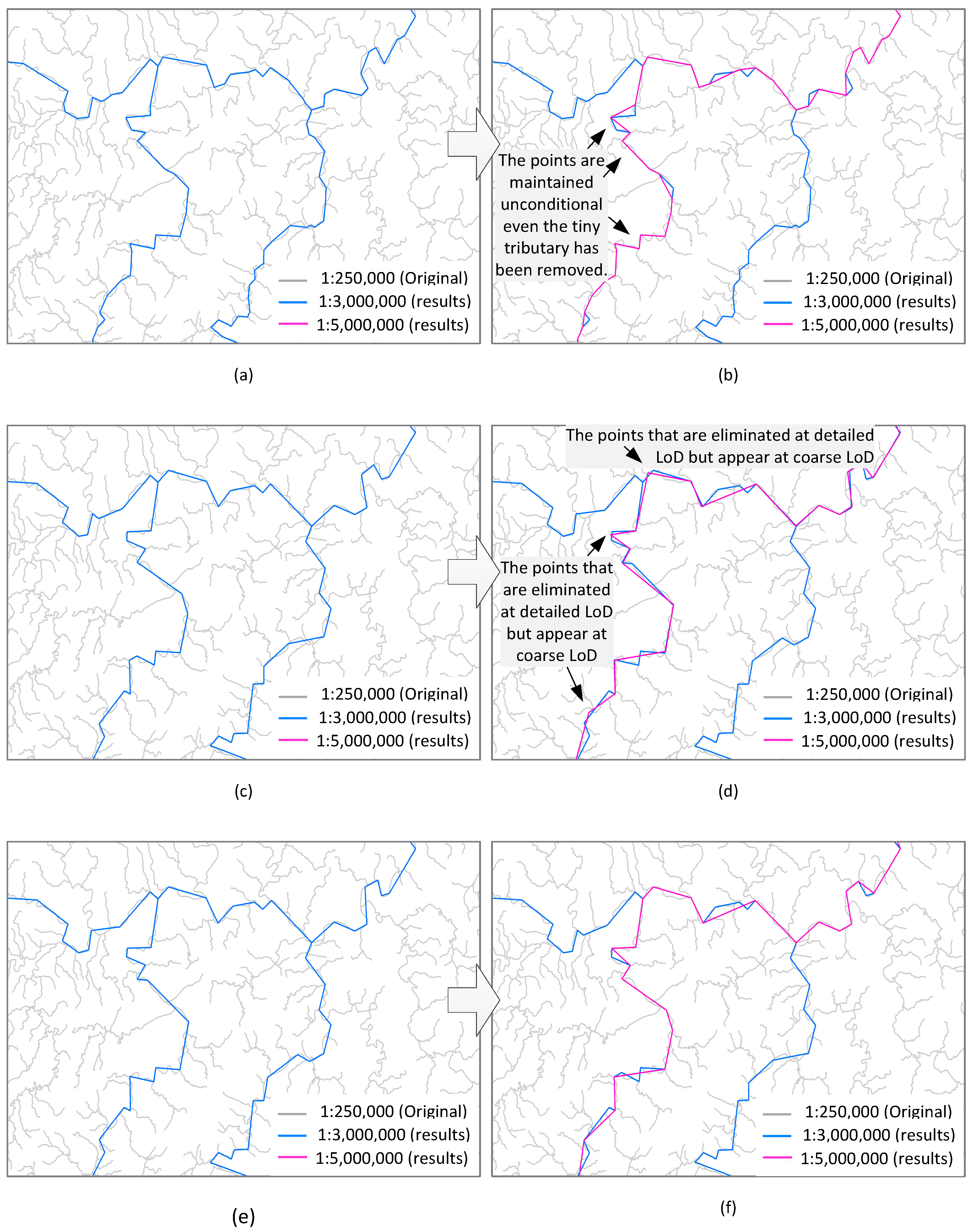
6.1. Generalization Quality

As the proposed matrix aimed to integrate network pruning and river simplification for the complex generalization of a river network, a comparison between the generalization between the matrix-based method and other approaches was undertaken. The compared methods included SelectSimpGen, which was to first select the rivers and then simplify the preserved river segments, and SimpleSelGen, which performed simplification before selection. All these methods used the same algorithms and parameters, and the only difference was that the multiple generalization operations were implemented either combined or in sequence.

The results of the complex generalization using the proposed matrix-based, SimpleSelGen and SelectSimpGen methods are illustrated in Figure 13, and observations were made from a detailed visual comparison. In the SimpleSelGen results, some unwanted linear jitters arose (Figure 13b), the reason being that this method first simplified river segments, then preserved the abstracted rivers for a given scale. To maintain the topological characteristics of the network, the points that connected tributaries to the mainstream were maintained unconditionally. This method may have also caused the issue of data redundancy as too many connecting points were maintained. As for the SelectSimpGen method, which uses the most common operation order in river generalization application [10,17,40], the results were also not satisfactory as the abstracted representations were not consistent. Some points appeared at a coarse LoD (1:1,000,000), but disappeared at a fine LoD (1:500,000) (Figure 13d). The matrix-based method provided better results than the other. On one hand, the generalized results showed good transformation when referring to the comprehensive process of network pruning and river simplification and the relationships between the rivers were well maintained without keeping unnecessary points. When a branch was removed, the point of the mainstream used to connect with the branch could be eliminated, if it did not overly describe the shape of river. On the other hand, the results illustrated a consistent generalization for continuous representation. The data at coarse LoD were the subset of that at the detailed LoD. This observation is also confirmed in

Table 1. Numerical evaluation of the generalized results by the proposed matrix-based method, SimpleSelectGen method and SelectSimpGen method.

	Length Compression (%)			Point Compression (%)			Ratio of New Points 1 (%)
	Matrix-Based	SimpleSelGen	SelectSimpGen	Matrix-Based	SimpleSelGen	SelectSimpGen	Matrix-Based	SimpleSelGen	SelectSimpGen
1:250,000	-	-	-	-	-	-	-	-	-
1:500,000	6.46	7.26	6.46	6.46	6.46	7.26	0	0	0
1:1,000,000	1.40	2.01	1.41	1.40	1.41	2.01	0	0	17.88
1:2,000,000	0.34	0.73	0.34	0.34	0.34	0.73	0	0	13.42
1:3,000,000	0.14	0.42	0.14	0.14	0.14	0.42	0	0	9.46
1:4,000,000	0.10	0.41	0.10	0.10	0.10	0.41	0	0	6.22
1:5,000,000	0.06	0.23	0.06	0.06	0.06	0.23	0	0	23.81
1:6,000,000	0.05	0.23	0.05	0.05	0.05	0.23	0	0	0

¹ The new point refers to the point that did not exist at a previous scale, but is present at the current scale. For instance, the SelectSimpGen method has 17.88% ratio of new points at 1:1,000,000, which means that there are 17.88% points that are not presented at 1:500,000.

, where some of the statistics are listed. Though all three methods had a similar length compression, the matrix-based method and SelectSimpGen method had a higher point compression. In contrast to the SelectSimpGen method, the matrix-based method did not create new points during the scale changes from detailed to coarse.

6.2. Data Storage

Note that the proposed matrix did not only provide guidance on integrating multiple generalizations, i.e., network pruning and river simplification, for the complex generalization of a river network, but also stored the variable LoDs using a vario-scale data structure. As a further step to evaluate the performance of the proposed matrix, we measured the time consumption of creating vario-scale data, the storage of vario-scale data, and the data retrieval for vario-scale representation.

Table 2. Performance of vario-scale data creation and data retrieval based on the matrix method in contrast to the Multiple Representation Database (MRDB). (a) Execution time of vario-scale data creation and the amount of data storage. (b) Execution time of vario-scale data retrieval and the data amount.

(a)
	Execution Time (s)		Data Amount (MB)
	Matrix-Based Method	MRDB 1	Matrix-Based Method	MRDB
Vario-scale	29.62	-	11.73	13.32
1:250,000	-	-	-	12
1:500,000	-	-	-	0.94
1:1,000,000	-	-	-	0.38
(b)
	Execution Time (s)		Data Amount (MB)
	Matrix-Based Method	MRDB	Matrix-Based Method	MRDB
1:250,000	0.18	2.3	8.9	12
1:500,000	0.46	0.12	1.05	0.94
1:1,000,000	0.07	0.06	0.02	0.38
1:2,000,000	0.05	-	0.05	-
1:3,000,000	0.04	-	0.02	-
1:4,000,000	0.03	-	0.02	-
1:5,000,000	0.03	-	0.02	-
1:6,000,000	0.03	-	0.02	-

¹ The compared river network data at 1:250,000, 1:500,000, and 1:1,000,000 was directly from the MRDB. The time consumption of data generation was unknown, because there was no record in the metadata.

shows the execution time of vario-scale data creation and the actual amount of data storage in comparison to the MRDB. It was observed that the total storage space of the vario-scale data was 11.73 MB, smaller than that of the MRDB, which was 13.32 MB with only three datasets of 1:250,000, 1:500,000 and 1:1,000,000 available. The time consumption to create the vario-scale data structure and retrieve the data for 1:500,000 and 1:1,000,000 was acceptable.

In addition, the matrix-based data set provided more scales than the MRDB, which only had three scales. According to the proposed matrix, the vario-scale data were stored with scale range (indicated by the importance range, as mentioned in Section 5), rather than a fixed scale. Furthermore, it was able to retrieve the data at any desired scale within the scale scope.

6.3. Scale Scope

Based on the scale correspondence, the rows of proposed matrix related to the river amount and indicated a set of discrete scales. The columns related to the simplification tolerance and led to a series of continuous scales. Therefore, it was easy to obtain the scale scope when a matrix was set for certain river network data.

Figure 14 illustrates the scale serial along the row and column of the matrix for the case study data. Theoretically speaking, the maximum scale is the scale of the original (source) data; the minimum scale is the map scale when there is only one river left. In this study, the scale scope was from 1:250,000 to 1:6,443,703. Note that the matrix did not support only fixed or limited number of scale. Any required scale within the scope was available through the interpolation calculation based on the scale scope.

7. Conclusions and Future Work

This study developed an integrated matrix that referred to complex generalization for the vario-scale representation of river networks. First, two linear LoDs, i.e., the LoDs of network pruning and river simplification were constructed and organized as rows and columns in a matrix hybrid. Then, correspondences between the map scale and the row/columns, as well as the scale linkage between the rows and columns of the matrix, were presented. Thus, the vario-scale LoDs were obtained by scanning the rows and columns in the matrix. The matrix model was validated by experimental evaluations, and the following conclusions were made:

• The proposed matrix fit the complex transformation of the river network, when different generalization operations, i.e., network pruning and river simplification, were involved (or any other generalization operators that could deliver data as a sequence of LoDs by setting appropriate parameters). Compared with traditional methods that conduct generalization operations in sequence, the matrix-base method provided the best results by integrating the operation in combination.
• Taking advantage of the proposed matrix, the LoDs data at an arbitrary scale were retrieved. In contrast to the MRDBs, where LoDs are stored as multiple versions separately and only limited scales are available, the storage of LoDs data based on a vario-scale matrix was much smaller.
• The proposed matrix enabled the vario-scale representation of a river network across a wide scale range. The large scale depended on the original data, which was used to establish the matrix. Theoretically, the smallest scale was the map scale when only one river was left.

In future work, several directions can be explored. First, the proposed matrix was established based on the linear LoDs hierarchies. In this study, the Douglas–Puecker algorithm was applied to construct the BLG tree for river simplification. Other algorithms, such as the Bend Simplify algorithm (which is widely adopted to simplify the United States National Hydrography [10,17]), can also be used. Efforts should be made to construct a bend-related LoDs hierarchies and the scale correspondence. Second, as network pruning and river simplification were assembled as two dimensions of the integrated matrix in this study, more generalization operations such as aggregation, displacement and smoothing may be appended to develop a high dimensional matrix for more complex data transformation. Third, the integrated matrix needs to be improved to be able to update (e.g., delete, insert and change) LoDs and propagate to all relevant scales. Fourth, though we only discussed the vario-scale matrix for a hydrographic network with a dendritic drainage pattern, it is possible to adapt it to hydrographic networks with other types of drainage patterns, or to extend it to other features such as roads and buildings. In addition, for content visualization where the objects of interest require considerable detail, while other coexisting objects do not require as much detail, the vario-scale matrix is a bright prospect in generating mixed-scale representation with a non-homogenous scale by mixing data at different LoDs [34].

References

1. Haklay, M.; Singleton, A.; Parker, C. Web mapping 2.0: The neogeography of the geoweb. Geogr. Compass 2008, 2, 2011–2039. [Google Scholar] [CrossRef]
2. Batty, M.; Hudson-Smith, A.; Milton, R.; Crooks, A. Map mashups, web 2.0 and the GIS revolution. Ann. GIS 2010, 16, 1–13. [Google Scholar] [CrossRef]
3. Jones, C.B.; Ware, J.M. Map generalization in the web age. Int. J. Geogr. Inf. Sci. 2005, 19, 859–870. [Google Scholar] [CrossRef]
4. Vrotsou, K.; Janetzko, H.; Navarra, C.; Fuchs, G.; Spretke, D.; Mansmann, F.; Andrienko, N.; Andrienko, G. Simplifly: A methodology for simplification and thematic enhancement of trajectories. IEEE Trans. Vis. Comput. Graph. 2015, 21, 107–121. [Google Scholar] [CrossRef] [PubMed]
5. Goodchild, M.F. Citizens as sensors: The world of volunteered geography. GeoJournal 2007, 69, 211–221. [Google Scholar] [CrossRef]
6. Regnauld, N.; McMaster, R.B. Chapter 3—A synoptic view of generalisation operators. In Generalisation of Geographic Information; Mackaness, W.A., Ruas, A., Sarjakoski, L.T., Eds.; Elsevier Science B.V.: Amsterdam, The Netherlands, 2007; pp. 37–66. [Google Scholar]
7. Foerster, T.; Stoter, J.; Kobben, B. Towards a formal classification of generalization operators. In Proceedings of the 23rd International Cartographic Conference, Moscow, Russia, 4–10 August 2007. [Google Scholar]
8. Stanislawski, L.V.; Buttenfield, B.P.; Bereuter, P.; Savino, S.; Brewer, C.A. Generalisation operators. In Abstracting Geographic Information in a Data Rich World: Methodologies and Applications of Map Generalisation; Burghardt, D., Duchêne, C., Mackaness, W., Eds.; Springer International Publishing: Cham, Switzerland, 2014; pp. 157–195. [Google Scholar]
9. Roth, R.E.; Brewer, C.A. A typology of operators for maintaining legible map designs at multiple scales. Cartogr. Perspect. 2011, 68, 29–64. [Google Scholar] [CrossRef]
10. Stanislawski, L.V. Feature pruning by upstream drainage area to support automated generalization of the united states national hydrography dataset. Comput. Environ. Urban Syst. 2009, 33, 325–333. [Google Scholar] [CrossRef]
11. Ai, T.; Ai, B.; Huang, Y. Multi-scale representation of hydrographic network data for progressive transmission over web. In Proceedings of the 24th International Cartographic Conference, Santiago, Chile, 15–21 November 2009. [Google Scholar]
12. Thomson, R.C.; Richardson, D.E. The ‘good continuity’ principle of perceptual organisation applied to the generalisation of road networks. In Proceedings of the 19th International Cartographic Conference, Ottawa, ON, Canada, 14–21 August 1999. [Google Scholar]
13. Ai, T. The drainage network extraction from contour lines for contour line generalization. ISPRS J. Photogramm. Remote Sens. 2007, 62, 93–103. [Google Scholar] [CrossRef]
14. Brewer, C.A.; Buttenfield, B.P. Framing guidelines for multi-scale map design using databases at multiple resolutions. Cartogr. Geogr. Inf. Sci. 2007, 34, 3–15. [Google Scholar] [CrossRef]
15. Cecconi, A.; Weibel, R.; Barrault, M. Improving automated generalisation for on-demand web mapping by multiscale databases. In Advances in Spatial Data Handling; Richardson, D., Oosterom, P., Eds.; Springer: Berlin/Heidelberg, Germany, 2002; pp. 515–531. [Google Scholar]
16. Neun, M.; Burghardt, D.; Weibel, R. Web service approaches for providing enriched data structures to generalisation operators. Int. J. Geogr. Inf. Sci. 2008, 22, 133–165. [Google Scholar] [CrossRef]
17. Buttenfield, B.P.; Stanislawski, L.V.; Brewer, C.A. Adapting generalization tools to physiographic diversity for the united states national hydrography dataset. Cartogr. Geogr. Inf. Sci. 2011, 38, 289–301. [Google Scholar] [CrossRef]
18. Stoter, J.; Post, M.; van Altena, V.; Nijhuis, R.; Bruns, B. Fully automated generalization of a 1:50k map from 1:10k data. Cartogr. Geogr. Inf. Sci. 2014, 41, 1–13. [Google Scholar] [CrossRef]
19. Touya, G.; Girres, J. Scalemaster 2.0: A scalemaster extension to monitor automatic multi-scales generalizations. Cartogr. Geogr. Inf. Sci. 2013, 40, 192–200. [Google Scholar] [CrossRef]
20. Töpfer, F.; Pillewizer, W. The principles of selection. Cartogr. J. 1966, 3, 10–16. [Google Scholar] [CrossRef]
21. Douglas, D.H.; Peucker, T.K. Algorithms for the reduction of the number of points required to represent a digitized line or its caricature. Cartogr. Int. J. Geogr. Inf. Geovis. 1973, 10, 112–122. [Google Scholar] [CrossRef]
22. Wang, Z.; Müller, J.C. Line generalization based on analysis of shape characteristics. Cartogr. Geogr. Inf. Syst. 1998, 25, 3–15. [Google Scholar] [CrossRef]
23. Ai, T.H.; Zhou, Q.; Zhang, X.; Huang, Y.F.; Zhou, M.J. A simplification of ria coastline with geomorphologic characteristics preserved. Mar. Geod. 2014, 37, 167–186. [Google Scholar] [CrossRef]
24. Van Oosterom, P. Semantic modelling an vario-scale geo-information. In Proceedings of the 5th International Workshop on Semantics and Conceptual Issues in Geographical Information Systems: SeCoGIS 2011, Brussels, Belgium, 1 November 2011. [Google Scholar]
25. Meijers, M.; Stoter, J.; Van Oosterom, P. Comparing the vario-scale approach with a discrete multi-representation based approach for automated generalisation of topographic data. In Proceedings of the 15th Workshop of the ICA commission on Generalisation and Multiple Representation, Istanbul, Turkey, 13–14 September 2012. [Google Scholar]
26. Sester, M.; Brenner, C. Continuous Generalization for Visualization on Small Mobile Devices; Springer: Berlin/Heidelberg, Germany, 2005; pp. 188–193. [Google Scholar]
27. Sester, M.; Brenner, C. A vocabulary for a multiscale process description for fast transmission and continuous visualization of spatial data. Comput. Geosci. 2009, 35, 2177–2184. [Google Scholar] [CrossRef]
28. Nöllenburg, M.; Merrick, D.; Wolff, A.; Benkert, M. Morphing polylines: A step towards continuous generalization. Comput. Environ. Urban Syst. 2008, 32, 248–260. [Google Scholar] [CrossRef]
29. Peng, D.; Wolff, A.; Haunert, J.-H. Continuous generalization of administrative boundaries based on compatible triangulations. In Geospatial Data in a Changing World: Selected Papers of the 19th Agile Conference on Geographic Information Science; Sarjakoski, T., Santos, M.Y., Sarjakoski, L.T., Eds.; Springer International Publishing: Cham, Switzerland, 2016; pp. 399–415. [Google Scholar]
30. Yang, B.; Purves, R.; Weibel, R. Variable-resolution compression of vector data. GeoInformatica 2008, 12, 357–376. [Google Scholar] [CrossRef]
31. Dilo, A.; van Oosterom, P.; Hofman, A. Constrained tgap for generalization between scales: The case of dutch topographic data. Comput. Environ. Urban Syst. 2009, 33, 388–402. [Google Scholar] [CrossRef]
32. Haunert, J.-H.; Dilo, A.; van Oosterom, P. Constrained set-up of the tgap structure for progressive vector data transfer. Comput. Geosci. 2009, 35, 2191–2203. [Google Scholar] [CrossRef]
33. Van Oosterom, P. Variable-scale topological data structures suitable for progressive data transfer: The gap-face tree and gap-edge forest. Cartogr. Geogr. Inf. Sci. 2005, 32, 331–346. [Google Scholar] [CrossRef]
34. Van Oosterom, P.; Meijers, M. Vario-scale data structures supporting smooth zoom and progressive transfer of 2d and 3d data. Int. J. Geogr. Inf. Sci. 2013, 28, 455–478. [Google Scholar] [CrossRef]
35. Huang, L.; Meijers, M.; Šuba, R.; van Oosterom, P. Engineering web maps with gradual content zoom based on streaming vector data. ISPRS J. Photogramm. Ermote Sens. 2016, 114, 274–293. [Google Scholar] [CrossRef]
36. Van Oosterom, P. A reactive data structure for geographic information systems. In Proceedings of the International Symposium on Computer-Assisted Cartography, Baltimore, MD, USA, 2–7 April 1989; pp. 665–674. [Google Scholar]
37. Van Oosterom, P. A storage structure for a multi-scale database: The reactive-tree. Comput. Environ. Urban Syst. 1992, 16, 239–247. [Google Scholar] [CrossRef]
38. Yang, W.; Li, J. A method for rapid transmission of multi-scale vector river data via the internet. Geod. Geodyn. 2012, 3, 34–41. [Google Scholar]
39. Harrie, L.; Weibel, R. Chapter 4—Modelling the overall process of generalisation. In Generalisation of Geographic Information; Ruas, A., Sarjakoski, L.T., Eds.; Elsevier Science B.V.: Amsterdam, The Netherlands, 2007; pp. 67–87. [Google Scholar]
40. Brewer, C.A.; Buttenfield, B.P.; Usery, E.L. Evaluating generalizations of hydrography in differing terrains for the national map of the united states. In Proceedings of the 24th International Cartographic Conference, Santiago, Chile, 15–21 November 2009. [Google Scholar]
41. Thomson, R.C.; Brooks, R. Efficient generalisation and abstraction of network data using perceptual grouping. In Proceedings of the 5th International Conference on GeoComputation, Ottawa, ON, Canada, 14–21 August 2000; pp. 23–25. [Google Scholar]
42. Sen, A.; Gokgoz, T.; Sester, M. Model generalization of two different drainage patterns by self-organizing maps. Cartogr. Geogr. Inf. Sci. 2014, 41, 151–165. [Google Scholar] [CrossRef]
43. Ai, T.; Liu, Y.; Chen, J. The hierarchical watershed partitioning and data simplification of river network. In Progress in Spatial Data Handling: 12th International Symposium on Spatial Data Handling; Riedl, A., Kainz, W., Elmes, G.A., Eds.; Springer: Berlin/Heidelberg, Germany, 2006. [Google Scholar]
44. Horton, R.E. Erosional development of streams and their drainage basins; hydrophysical approach to quantitative morphology. Geol. Soc. Am. Bull. 1945, 56, 807–813. [Google Scholar] [CrossRef]
45. Dong, P. Generating and updating multiplicatively weighted voronoi diagrams for point, line and polygon features in gis. Comput. Geosci. 2008, 34, 411–421. [Google Scholar] [CrossRef]
46. Gökgöz, T.; Sen, A.; Memduhoglu, A.; Hacar, M. A new algorithm for cartographic simplification of streams and lakes using deviation angles and error bands. ISPRS Int. J. Geo-Inf. 2015, 4, 2185–2204. [Google Scholar] [CrossRef]
47. Ai, T.; Ke, S.; Yang, M.; Li, J. Envelope generation and simplification of polylines using delaunay triangulation. Int. J. Geogr. Inf. Sci. 2016, 31, 1–23. [Google Scholar] [CrossRef]
48. Shi, W.; Cheung, C.K. Performance evaluation of line simplification algorithms for vector generalization. Cartogr. J. 2006, 43, 27–44. [Google Scholar] [CrossRef]
49. Meijers, M. Variable-Scale Geo-Information. Ph.D. Thesis, Delft University of Technology, Delft, The Netherlands, 16 December 2011. [Google Scholar]
50. Li, Z.; Openshaw, S. Algorithms for automated line generalization based on a natural principle of objective generalization. Int. J. Geogr. Inf. Sci. 1992, 6, 373–389. [Google Scholar] [CrossRef]
51. Li, Z.; Openshaw, S. A natural principle for objective generalization of digital map data. Cartogr. Geogr. Inf. Syst. 1993, 20, 19–29. [Google Scholar] [CrossRef]
52. Muller, J.C. Optimum point density and compaction rates for the representation of graphic lines. In Proceedings of the Eighth International Symposium on Computer-Assisted Cartography, Baltimore, MD, USA, 29 March–3 April 1987. [Google Scholar]
53. Chen, J.; Hu, Y.; Li, Z.; Zhao, R.; Meng, L. Selective omission of road features based on mesh density for automatic map generalization. Int. J. Geogr. Inf. Sci. 2009, 23, 1013–1032. [Google Scholar] [CrossRef]
54. Li, Z.; Zhou, Q. Integration of linear and areal hierarchies for continuous multi-scale representation of road networks. Int. J. Geogr. Inf. Sci. 2012, 26, 855–880. [Google Scholar] [CrossRef]
55. Amos, T. Features of similarity. Psychol. Rev. 1977, 84, 327–352. [Google Scholar]
Figure 1. The vario-scale representation of river network. (Note that the adjacent points of any two river branches were maintained to preserve the topological relations between adjacent branches).
Ijgi 06 00218 g001
Figure 2. The results of iterative merging based on hierarchical partitioning of the river catchment. (a) Rivers labeled with the Horton code. (b) Watershed partition based on the linear constrained Voronoi diagram. (c) Intermediate result that watershed area corresponding to the lowest-order label merged iteratively with the one which had a higher order label. (d) The final merging result.
Ijgi 06 00218 g002
Figure 3. An example of a river network and the stepwise network pruning (Length means the length of the eliminated river drawn in magenta; Area means the corresponding watershed area; Order refers to the Horton code; and Step refers to the order in the process of pruning. Pruning considered the length, area, and Horton order of rivers together rather than by a single hydrographic factor. For example, the river eliminated at Step 7 was longer than that at Step 10, and the one eliminated at Step 8 had a larger watershed area than that at Step 9).
Ijgi 06 00218 g003
Figure 4. Linear hierarchy for the generalization process based on the stepwise pruning of the river network. For each step, the least important river was eliminated, and the adjacent segments of the preserved rive were merged, e.g., r1, r4 and r11).
Ijgi 06 00218 g004
Figure 5. Binary Line Generalization (BLG) trees for the generalization process based on river simplification. (a) Shape-describing points retrieved from rivers. (b) BLG trees for LoDs representation of the rivers.
Ijgi 06 00218 g005
Figure 6. Reconstructing representation at certain levels of detail (LoDs).
Ijgi 06 00218 g006
Figure 7. Linear BLG trees of r1 and the simplification process by selecting points from the linear BLG tree. For a given scale, if the river r1 is preserved, the primary head-water points of involved segments will always be retained. Others will be selected from left to right in the linear BLG trees using the simplification tolerance. To generate a desired LoD representation, the selected points are adjusted in the correct sequence as in the original line.
Ijgi 06 00218 g007
Figure 8. The complex generalization of a river network. (a) The original river network. (b) Intermediate generalized result when river BF was eliminated and the preserved revers were simplified. (c) Intermediate generalized result when river CE was eliminated and the preserved revers were simplified. (d) The generalized result when only river DA was preserved and simplified.
Ijgi 06 00218 g008
Figure 9. The matrix hybrid constructing the complex generalization of river network.
Ijgi 06 00218 g009
Figure 10. Deriving LoDs by scanning the matrix hybrid. (Progressive network pruning and river simplification were conducted by expending the area in vertical and horizontal dimensions of the matrix).
Ijgi 06 00218 g010
Figure 11. Appropriate parameter L of the sample river network.
Ijgi 06 00218 g011
Figure 12. Tables and relationships of vario-scale data structure based on the matrix.
Ijgi 06 00218 g012
Figure 13. The generalized results using the matrix-based method, SimpleSelGen method and SelectSimpGen method. The original data are presented with grey in the background. (a) Generalized result by the SimpleSelGen method, 1:3,000,000. (b) Generalized result by the SimpleSelGen method, 1:5,000,000. (c) Generalized result by the SelectSimpGen method, 1:3,000,000. (d) Generalized result by the SelectSimpGen method, 1:5,000,000. (e) Generalized result by the matrix-based method, 1:3,000,000. (f) Generalized result by the matrix-based method, 1:5,000,000.
Ijgi 06 00218 g013
Figure 14. The experimental scale scope of matrix based on the river network data of the case study. (a) The series of scales along row of matrix; and (b) the series of scales along column of matrix.
Ijgi 06 00218 g014