GeoSpark SQL: An Effective Framework Enabling Spatial Queries on Spark


1
Institute of Remote Sensing & GIS, Peking University, Beijing 100871, China
2
Beijing Advanced Innovation Center for Future Internet Technology, Beijing 100124, China
3
Faculty of Information Engineering, China University of Geosciences, Wuhan 430074, China
4
Collaborative Innovation Center of eTourism, Institute of Tourism, Beijing Union University, Beijing 100101, China
5
State Key Laboratory of Resources and Environmental Information System, Institute of Geographical Sciences and Natural Resources Research, Chinese Academy of Sciences, Beijing 100101, China
*
Author to whom correspondence should be addressed.
ISPRS Int. J. Geo-Inf. 2017, 6(9), 285; https://doi.org/10.3390/ijgi6090285
Submission received: 24 July 2017
/
Revised: 1 September 2017
/
Accepted: 6 September 2017
/
Published: 8 September 2017
Abstract
:In the era of big data, Internet-based geospatial information services such as various LBS apps are deployed everywhere, followed by an increasing number of queries against the massive spatial data. As a result, the traditional relational spatial database (e.g., PostgreSQL with PostGIS and Oracle Spatial) cannot adapt well to the needs of large-scale spatial query processing. Spark is an emerging outstanding distributed computing framework in the Hadoop ecosystem. This paper aims to address the increasingly large-scale spatial query-processing requirement in the era of big data, and proposes an effective framework GeoSpark SQL, which enables spatial queries on Spark. On the one hand, GeoSpark SQL provides a convenient SQL interface; on the other hand, GeoSpark SQL achieves both efficient storage management and high-performance parallel computing through integrating Hive and Spark. In this study, the following key issues are discussed and addressed: (1) storage management methods under the GeoSpark SQL framework, (2) the spatial operator implementation approach in the Spark environment, and (3) spatial query optimization methods under Spark. Experimental evaluation is also performed and the results show that GeoSpark SQL is able to achieve real-time query processing. It should be noted that Spark is not a panacea. It is observed that the traditional spatial database PostGIS/PostgreSQL performs better than GeoSpark SQL in some query scenarios, especially for the spatial queries with high selectivity, such as the point query and the window query. In general, GeoSpark SQL performs better when dealing with compute-intensive spatial queries such as the kNN query and the spatial join query.
1. Introduction
In recent years, due to the rapid development of the Internet, human society has entered an era of information explosion, and the amount of information is rapidly growing at an unimaginable speed. Hence, the demand for storage and processing of massive data is also increasing. A large amount of data is aggregated together and brings big challenges to the data processing, analysis and mining. That is the background of so-called “big data”. Currently, big data is attracting more and more attention, and quickly becomes a research hotspot in both academia and industry.
As to the geographic information industry, a large amount of location-related spatial data is produced every day in the context of the rapid development of geospatial information services such as various LBS apps (e.g., Google Maps, Baidu Map). On the one hand, a single server node has been gradually unable to meet the needs of both massive spatial data management and query performance. On the other hand, a large number of concurrent user requests against the backend geographic information services bring a huge load stress. In order to deal with large-scale spatial queries efficiently, clusters are required to process decentralized and massive spatial data [1]. Therefore, the spatial query processing technique in the cluster environment has become a critical issue in the big spatial data era.
Meanwhile, it has been widely believed that the traditional relational database is not extensible and unable to handle huge amounts of data due to restrictions of the ACID (Atomicity, Consistency, Isolation, Durability) and SQL (Structured Query Language) features [2]. With the rapid development of cloud computing, the database has entered the era of NoSQL, which is built on cloud clusters. Unlike the traditional database, the NoSQL database discards the ACID features and achieves massive data storage and management through distributed processing.
The NoSQL database has become a popular data management tool in the cloud-computing environment. Its embedded MapReduce framework is considered a simple but very efficient parallel computing architecture. As for the GIS industry, there was some research successfully using NoSQL and MapReduce technologies in spatial data storage and query processing. For example, Chen et al. used Hadoop to implement a cloud-based spatial data storage system [3]. Liu et al. applied MapReduce in the optimization of kNN (k-Nearest Neighbor) spatial queries [4]. ESRI (Environmental Systems Research Institute) developed the ESRI Geometry API for Java, and then implemented the Spatial Framework for Hadoop [5] integrating ArcGIS with Hadoop by registering spatial query functions in Hive. Data processing capabilities are thus improved through parallel spatial queries against the Hadoop distributed file system (Hadoop Distributed File System, HDFS) [6,7,8,9,10,11,12]. However, because in the MapReduce process a lot of I/O operations would be produced [13,14,15], real-time large-scale spatial data processing is difficult to achieve.
Spark [16], which was born in 2009 at the Berkeley Algorithms, Machines and People Lab, University of California, has now become a top open source project of the Apache Software Foundation. Spark is a distributed memory-based big data computing framework [17]. The distributed memory-based design improves real-time data processing in the big data environment, while ensuring high fault tolerance and high scalability. The most important thing is that users can quickly deploy Spark in a large number of cheap computers to form a computing cluster.
There were some preliminary studies on applying Spark in spatial queries. Xie et al. compared the difference in the query efficiency through constructing a quadtree and an R-tree on Spark [18], but the Spark used is also an earlier version, and there are obvious usage restrictions by declaring different RDD (Resilient Distributed Dataset) sets on the data storage. Wen et al. used JTS (Java Topology Suite) to achieve spatial enabled UDF (User Defined Function) in Spark and compared the query efficiency with the approach using PostGIS as the storage backend [19], but the study did not take full advantage of Spark’s memory computing features. The SpatialSpark [20] project achieved accelerating parallel processing of spatial data through a partitioning indexing method based on the Spark broadcast mechanism. GeoSpark [21] implemented the spatial resilient distributed datasets (SRDD) to enable spatial query processing in the Spark. Similar Spark-based spatial query systems also include Spark-GIS [22], Magellan [23], GeoTrellis [24] and LocationSpark [25]. In addition, some scholars studied the issues of high-performance spatial join queries based on Spark [26,27].
However, in the aforementioned studies, users had to organize their own Spark Scala scripts when submitting spatial queries, which brought operation inconvenience. Writing Scala scripts requires professional developing experience, thus leading to the difficulty in using spatial query systems for ordinary users. A common interface, such as SQL, is very necessary and user-friendly for spatial queries, but the traditional RDBMS-based spatial database like PostGIS/PostgreSQL is unable to meet the needs of both massive spatial data management and query performance. Hence, in order to address the increasingly large-scale spatial query processing requirement under the era of big data, we propose an effective framework GeoSpark SQL, which enables spatial queries on Spark. On the one hand, GeoSpark SQL provides a convenient SQL interface; on the other hand, GeoSpark SQL achieves both efficient storage and high-performance parallel computing through integrating Hive and Spark.
2. Design Issues
Compared with the traditional MapReduce computing framework like Hadoop, Spark has the advantage of memory computing, and is thus considered a new generation of the MapReduce computing framework [28]. Existing studies also demonstrate that Spark has the potential to become an excellent spatial data management and computing framework [18,19,20,21,22,23,24,25,26,27]. Therefore, we expect to explore a Spark-based spatial query implementation framework i.e., GeoSpark SQL, to provide a convenient SQL query interface, and to achieve high-performance computing at the same time. Providing an effective spatial query infrastructure in the distributed computing environment would greatly facilitate various spatial information applications.
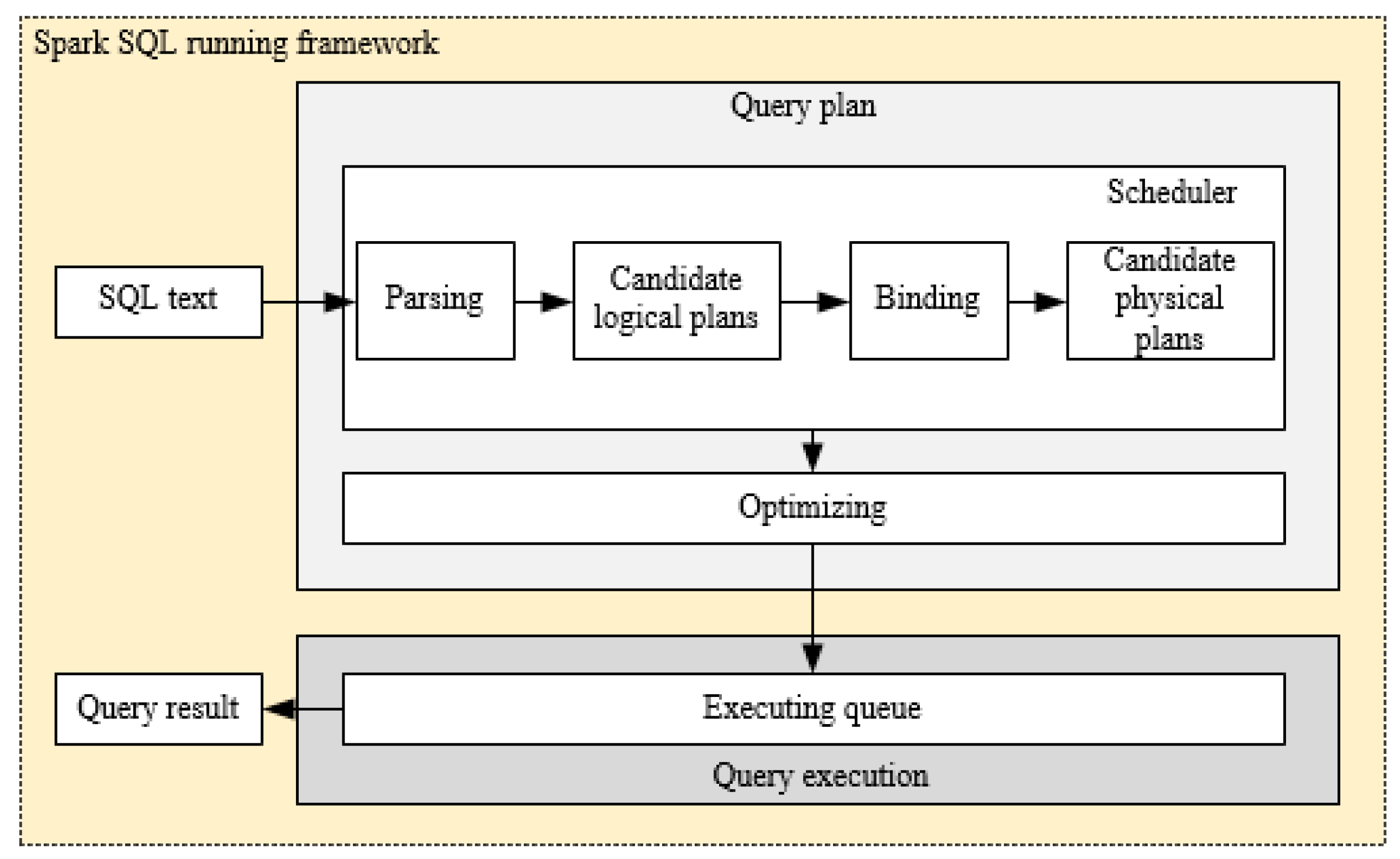
Spark SQL is a widely used component of Spark for processing the structured data. Spark SQL’s predecessor is Shark, and it tries to provide a quick start tool for the technical staff who are familiar with RDBMS and are not particularly skilled in MapReduce. In fact, there are some early SQL-on-Hadoop tools running on Hadoop, such as Drill, Impala and Shark [29,30,31]. However, the large numbers of intermediate disk I/O operations in the MapReduce process are the major bottleneck of the query tasks, and the limited performance of disks reduces the query efficiency. In order to achieve higher efficiency, the SQL-on-Spark tool began to emerge, and Spark SQL was born under this context. Similar to the relational database, the SQL query statement in Spark SQL is also mainly composed of projection (e.g., a1, a2, a3), data source (e.g., tableA), and filter (i.e., conditions) [32]. The running framework of Spark SQL is shown in Figure 1. After the SQL query is interpreted, a series of candidate physical plans are generated through binding data and calculation resources. Then, an optimization process is performed to choose an optimal plan put into the executing queue. Lastly, the query result would be returned after the execution step.
Therefore, we can take full advantage of Spark SQL to achieve our spatial query processing framework, i.e., GeoSpark SQL. However, Spark SQL cannot be used directly for spatial queries, several problems should be addressed through extending Spark SQL. First, because Spark including Spark SQL is only a memory-computing framework, there is a need to design an appropriate spatial data external storage method as well as the spatial index. Secondly, Spark SQL does not support spatial functions or operations, so it is necessary to extend spatial operators in the Spark environment to meet the spatial query requirement. Finally, besides the internal query optimizer provided by Spark SQL, an external spatial query optimizer could be designed to achieve plan optimization for spatial queries to improve performance. Figure 2 illustrates the architecture of GeoSpark SQL.
Spatial data is stored in the external storage such as Hive, and when the spatial query is submitted GeoSpark SQL would read the spatial data into memory, perform spatial operations and obtain query results. Under the GeoSpark SQL framework, the spatial query processing workflow is as follows: (1) The spatial query in form of SQL statement is parsed by the Spark SQL built-in SQL parser to build up a syntax tree, in which key words such as SELECT, FROM and WHERE, expressions, projections, and data sources are all separated and thus the machine could “understand” the semantics of the spatial query. (2) The SQL statement is bound to concrete resources in the spatial data schema (columns, tables, views, etc.), and this step is done by Spark SQL as well. (3) After Spark SQL provides several candidate execution plans, its internal query optimizer chooses an optimal plan according to running statistics, and then the external spatial query optimizer would further optimize the physical spatial query plan, especially using the strategy of reducing I/O costs with the help of the spatial index to improve query performance. (4) Finally, in the execution stage, the physical query plan is scheduled and executed in the order of “operation -> data source -> result” with the support of the extended spatial UDFs (user defined functions). In memory, the spatial query result is in the form of Dataframe objects. Dataframe, as a typical data structure in Spark, is an RDD-based distributed data set, which is similar to the traditional database’s two-dimensional relational table.
3. Storage Management
3.1. Hive-Based Spatial Data Storage
Since Spark is just a memory-computing framework, there is a need to choose the appropriate external storage source. Currently, Spark enables connecting many external storages such as Hadoop HDFS, Parquet and Hive. Hive is a popular data warehouse that supports managing large data sets and provides HQL interfaces for users. It provides a rich set of options to store and manage relational data, and Spark can quickly import data and metadata from Hive. Hive’s internal data redundancy and fragmentation mechanisms result in a high-reliability and high-performance data management solution. In addition, its indexing mechanism makes data I/O performance greatly improved.
Spark has built-in support for Hive, and in fact the Spark SQL project was originally built on Hive as the storage side. Compared with other data management approaches, such as Hadoop HDFS and Parquet, which store data in files, Hive’s index makes Spark only read the data and meet user-defined conditions, and thus speeds up data I/O greatly. Moreover, metadata or schema information can also be obtained from Hive directly, avoiding the complexity of manually defining the data structure in Spark. Hence, using Hive as the external storage in Spark based spatial data management is a reliable design.
According to the above considerations, we design and implement the following technical process to convert the representative spatial data format (i.e., shape file) into Hive and Spark, which reveals the universal steps to import spatial data into the Hive/Spark environment.
(1) Read the geometry objects in the shape file through the ESRI Geometry API and write them into a text file, separating the attributes by Tabs for each geographic feature.
(2) Use the CREATE TABLE statement to build the spatial data table in the Hive, specifying the data source as the Tab-separated text file. After this step, the spatial data could be used in Hive.
(3) Start Hive’s metastore service, and then submit a SQL statement which queries the full table through HiveContext in the Spark, obtaining a Dataframe object that includes both the spatial data table and the schema information.
(4) Set the storage level of the Dataframe object as MEMORY_ONLY, and perform the collect action to load the Hive data into the Spark memory. Then the spatial data is successfully imported into Spark and subsequent computing or analysis could be performed.
3.2. Data Structure in the Spark Memory
The spatial data in the external storage Hive is imported into the Spark memory, in the form of Dataframe objects. Dataframe is a new type of data structure beginning with Spark version 1.3.0, and is renamed from the past SchemaRDD [16]. In Spark, Dataframe is an RDD-based distributed data set, similar to the traditional database’s two-dimensional relational table. Dataframe is able to be constructed from a variety of data sources, such as Hive tables, external relational databases, RDDs generated through Spark calculation, and so on.
Compared with the generalized RDD, Dataframe’s difference is with schema metadata, that is, Dataframe is represented by the two-dimensional table, and each column has its own name and type. This allows the Spark SQL to gain insight into the structure of the information, so as to optimize the Dataframe transformation of the targeted data source, and ultimately achieve a substantial increase in query efficiency. Hence, Using Dataframe as the memory data structure of the geographical feature facilitates the original data conversion and usage. In addition, the excellent performance of Spark would help to achieve an efficient spatial query framework.
Because of Spark’s column-based memory storage feature, when the query operation is performed, not all data but parts are read, being filtered by the specific column. In addition, compression algorithms are used so that the throughput rate of the filter operation is improved to a higher level. In a simple sense, it is assumed that the column-based memory storage has set up an inverted index for each column.
3.3. Spatial Index Design
In order to minimize the I/O cost from the Hive-based external storage to the Spark memory, we design a spatial indexing method in the GeoSpark SQL framework. When the Hive table is initiated, the MBR (Minimum Bounding Rectangle) of the geographic feature, in the form of four additional table fields (i.e., xmin, xmax, ymin and ymax), is generated. Then, when the spatial query is submitted, the MBR of the feature is used to trigger the filtering operation, that is, the geographical feature whose MBR is not overlapped with the user-defined spatial range will not be loaded into the Spark memory. This spatial indexing method is actually a simple but very effective approach by extending the MBR fields in Hive tables, utilizing Hive’s own indexing and filtering functions, and thus effectively reducing both the deserialization overhead and the topological calculation overhead.
4. Spatial UDFs
4.1. UDF Utility of Spark
Spark 1.1 introduced the UDF utility, that is, users can customize the required UDF to process data in Spark. Because now the built-in functions supported by Spark are quite limited and none-spatial, it is of great importance to use UDF to extend and implement the needed spatial functions, i.e., the so-called spatial UDFs.
Spark UDF is actually in form of Scala function, which is encapsulated as an “Expression” node by the parser catalyst, and finally the result of the UDF is calculated by the “eval” method based on the current column. Moreover, UDFs can appear either in SELECT columns or in WHERE and JOIN ON conditions.
Currently Spark uses Hive SQL Parser as the SQL parser, so users can register UDF either through SQLContext or with the SQL statement, beginning with “CREATE TEMPORARY FUNCTION”. However, because Hive only supports equivalent joins, UDF cannot be used directly in JOIN conditions, while UDF is able to be submitted through calling the “callUDF” function in Spark.
4.2. Spatial Operators
The Open Geospatial Consortium (OGC) defines a set of standard data types and operators for spatial SQL to achieve interoperability between different spatial databases and other spatial data management tools. Most of these spatial functions start with the prefix “ST_”. According to the spatial query operators defined in the standard ISO/IEC 13249-3:2016 (SQL/MM-Spatial) [33], we implement the following Spark-based UDF functions as shown in Table 1. The ESRI Spatial Framework for Hadoop also has implemented the relevant spatial functions based on Hive. In addition, the traditional spatial database PostGIS/PostgreSQL has built-in spatial operators as well. Therefore, we use the two as the benchmark for spatial query testing. From Table 1, it is observed that except for the ST_Relate function, the UDF functions all receive two spatial features as input arguments and return a ‘Boolean’ value.
5. External Spatial Query Optimizer
5.1. Query Acceleration Based on Spatial Index
It is very time consuming to perform topological calculations and deserialization operations that transform the binary data into in-memory feature objects when processing spatial queries. In order to reduce the deserialization and topological calculation cost, the spatial index (i.e., MBRs of the spatial features) is used to filter unnecessary spatial features that do not intersect with the user-defined spatial range. Hence, in the external query optimization stage, we need to identify the user-defined spatial range in form of MBR, and re-write the SQL statement through adding conditions filtering the objects that do not intersect with the MBR.
For instance, if we submit a simple spatial query organized as the SQL statement “SELECT * FROM polygon_set WHERE ST_Intersects(geometry, ‘POLYGON((0 0,0 1,1 1,1 0,0 0))’);”, the MBR of “POLYGON((0 0,0 1,1 1,1 0,0 0))” is calculated as {xmin = 0, ymin = 0, xmax = 1, ymax = 1}, and the original SQL statement is re-written as the following:
SELECT * FROM polygon_set
WHERE xmin <= 1.0 AND xmax >= 0.0 AND ymin <= 1.0 AND ymax >= 0.0 AND ST_Intersects(geometry, ‘POLYGON((0 0,0 1,1 1,1 0,0 0))’);
It is observed that the filtering conditions “xmin <= 1.0 AND xmax >= 0.0 AND ymin <= 1.0 AND ymax >= 0.0” are added into the transformed SQL statement to ensure only the features which are possible to intersect with the MBR {xmin = 0, ymin = 0, xmax = 1, ymax = 1} would be loaded into memory, thus reducing the deserialization overhead and the topological computation overhead.
In the above filtering conditions, xmin, ymin, xmax and ymax are just the added fields in the Hive’s spatial data table according to our spatial index design. In fact, through extending the MBR fields in Hive tables and adding filtering conditions in the transformed SQL statement, Hive’s own none-spatial index is activated to accomplish spatial filtering functions. Hence, our index-based query acceleration approach is a simple but efficient design, which facilitates reducing the I/O cost as much as possible in the initial stage.
5.2. Object Deserialization Cache
Besides the spatial index-based query acceleration method, we design a spatial object deserialization cache approach to further reduce the deserialization cost and accelerate spatial query processing.
In the coding process, we use the local cache object in the Google Guava package for spatial feature deserialization. The cache object consists of a key-value pair, where the key is the hash value generated by the hash method of the java.nio. ByteBuffer class, receiving the binary array of the spatial feature, and the value is the deserialized “Geometry” object. Parameters like the size of the cache are determined by the actual hardware configuration. If the memory of the server is large, it can be set to a larger cache. Otherwise, it needs to be set to a smaller cache to avoid Out of Memory Error.
6. Experimental Evaluation
6.1. Experimental Platforms
Because currently there is no spatial query system like GeoSpark SQL that enables SQL-based spatial queries in Spark, we choose the classic Hadoop-based spatial query system, ESRI Spatial Framework for Hadoop, as the experimental benchmark. ESRI Spatial Framework for Hadoop is an open source project hosted on Github and is easy to install, use and test. Most importantly, ESRI Spatial Framework for Hadoop as a distributed spatial query system also supports SQL-based spatial queries. In addition, in order to illustrate the difference between GeoSpark SQL and the traditional none-distributed spatial database, we compare with PostGIS/PostgreSQL in spatial query performance as well.
Hence, after implementing GeoSpark SQL, we deploy it as well as ESRI Spatial Framework for Hadoop onto a computing cluster that hosts on Meituan Cloud (https://www.mtyun.com/). Moreover, PostGIS/PostgreSQL is also deployed on a single server. We carry out spatial queries on GeoSpark SQL and compare the query performance with the other two software platforms. Configuration details of the platforms are listed in Table 2:
6.2. Data Description
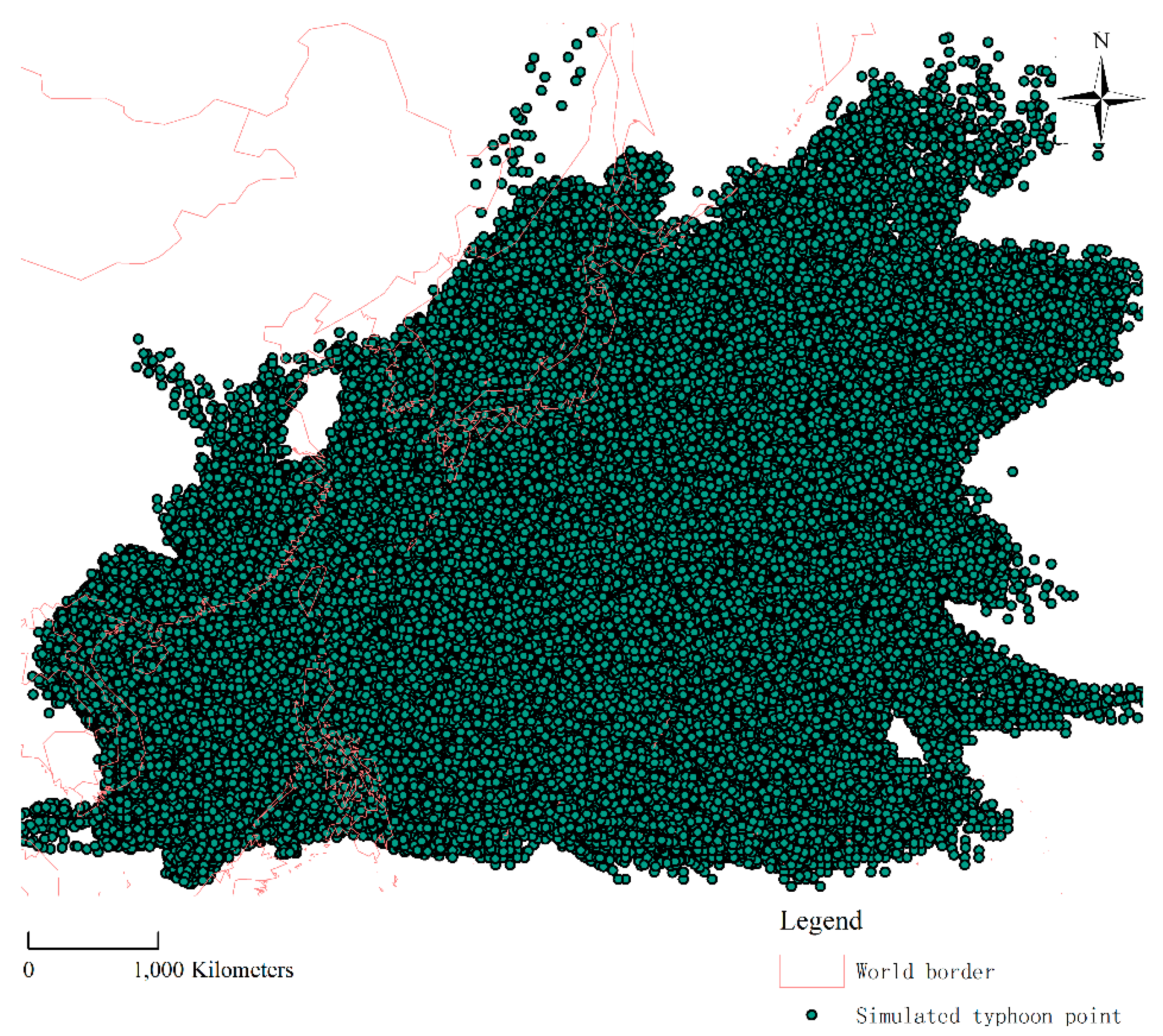
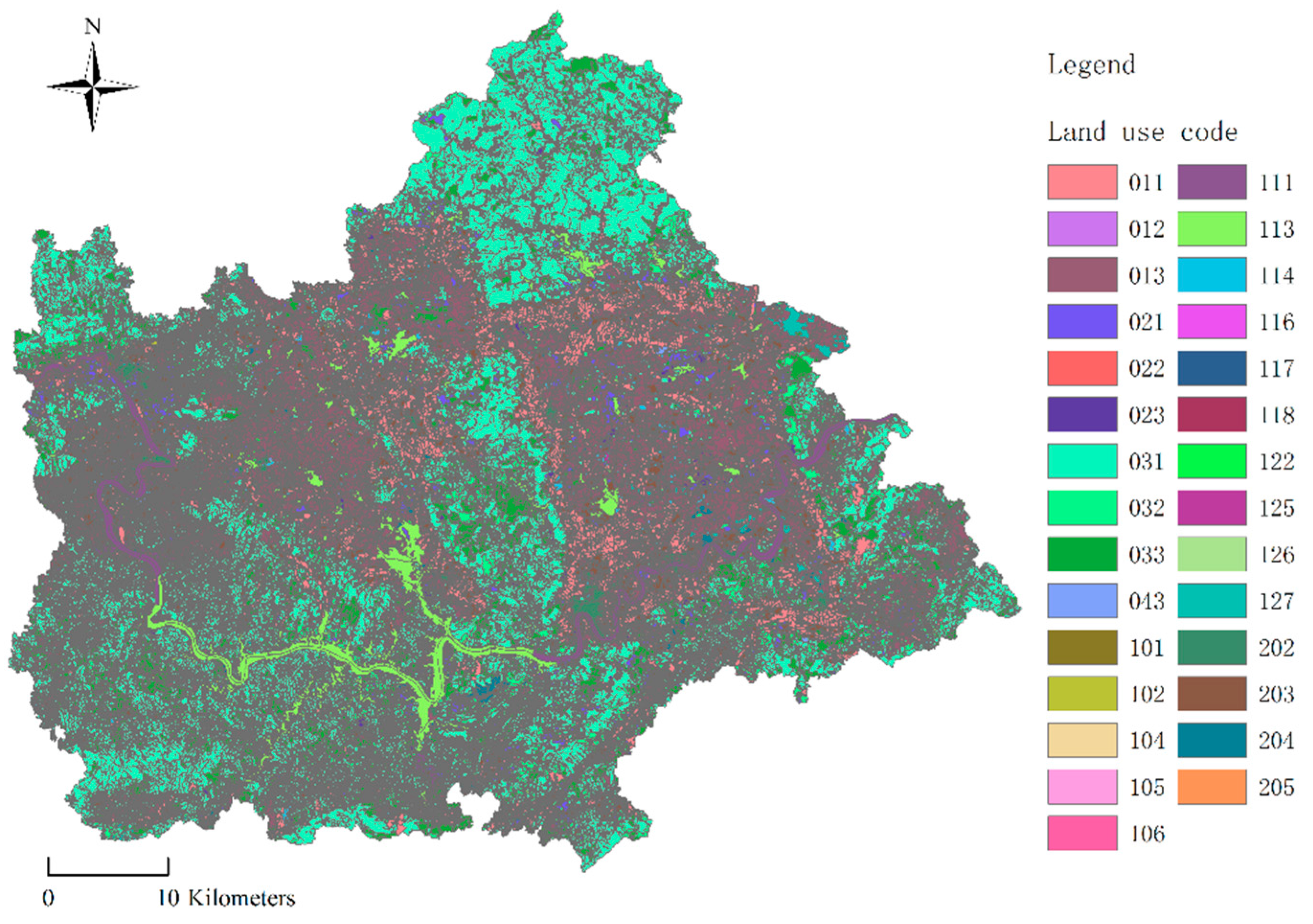
For a more comprehensive test of the spatial query performance on the database platforms, two spatial datasets were prepared. The one is the simulated point dataset of northwest pacific typhoon routes for 5000 years and the other is the land use dataset of Zhenlong Town, Heng County, Nanning City, Guangxi Province of China. Table 3 illustrates detailed descriptions of the two test datasets, and Figure 3 and Figure 4 show the visualized geographic maps of the two test datasets.
Moreover, the “shp2pgsql” tool is utilized to import the two spatial datasets into PostGIS/PostgreSQL. We also import the spatial datasets into Hive and Spark according to the storage management approaches as described in Section 3. Then, we use GIST (Generalized Search Trees) to build the spatial index in PostGIS / PostgreSQL through submitting the following statement “CREATE INDEX [index_name] ON [table_name] USING GIST ([geometry_field_name])”, and the spatial index in GeoSpark SQL is built through the method described in Section 3.3.
6.3. Experimental Results
The test cases are designed to cover as many spatial query types as possible. They include attribute query, kNN (k-Nearest Neighbor) query, point query, window query, range query, directional query, topological query and multi-table spatial join query. Except for the difference in the record order, it is observed that all of the query results under different database platforms are exactly the same, which illustrates that GeoSpark SQL works properly. In our experiment, each test case has been run 10 times and the average time cost is taken for performance evaluation. Query statement, query type, number of results and average costs in different experimental platforms are all listed to make the evaluation more objectively.
6.3.1. Attribute Query
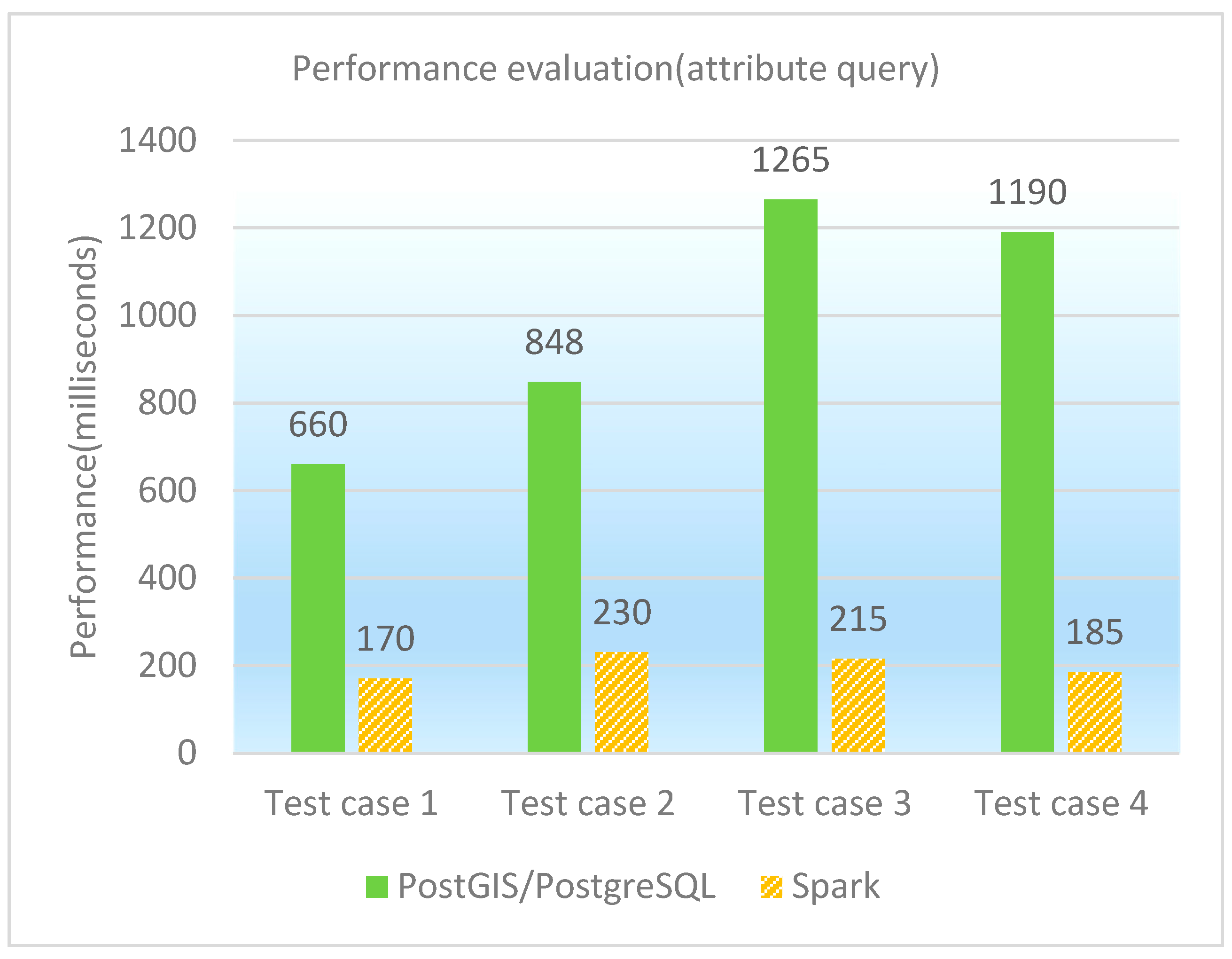
The attribute query is one of the most popular queries in the spatial database, although it does not involve spatial operators. Four test cases as attribute queries are designed and performed on PostGIS/PostgreSQL, GeoSpark SQL and ESRI Spatial Framework for Hadoop, respectively. The concrete test cases are in Table 4:
The performance of testing attribute queries under different database platforms is shown in both Table 5 and Figure 5. Because the query performance on ESRI Spatial Framework for Hadoop is much slower than the other two database platforms, we just list the latter two when drawing the performance comparison figure (i.e., Figure 5). It is observed that GeoSpark SQL is better than PostGIS/PostgreSQL and ESRI Spatial Framework for Hadoop in attribute query performance.
6.3.2. kNN Query
The kNN (k-Nearest Neighbor) query enables finding the nearest k points as well as their attributes from a given point. Two test cases as kNN queries are designed and performed on PostGIS/PostgreSQL, GeoSpark SQL and ESRI Spatial Framework for Hadoop, respectively. The concrete test cases are illustrated in Table 6, and the performance of kNN queries under different database platforms is shown in both Table 7 and Figure 6. It is observed that GeoSpark SQL is much better than PostGIS/PostgreSQL and ESRI Spatial Framework for Hadoop in kNN query performance.
6.3.3. Point Query
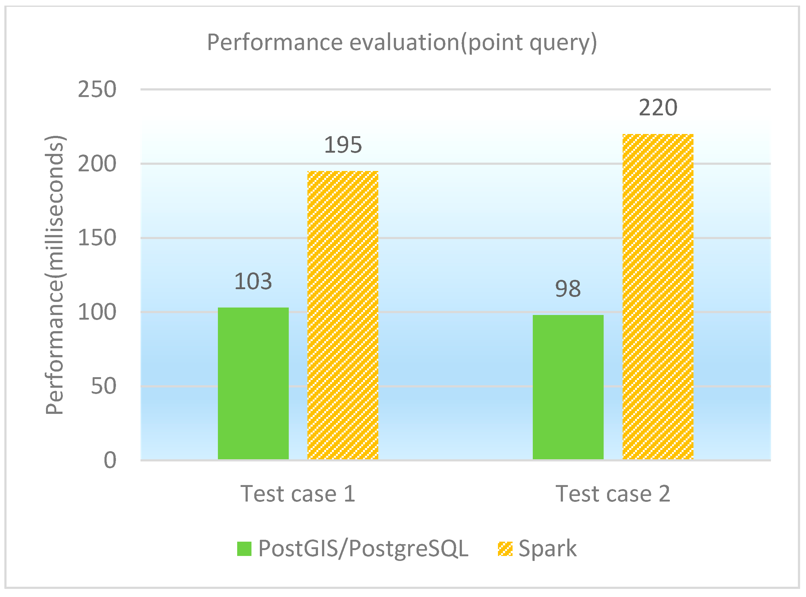
The point query is to find the features that contain the given point. Two test cases as point queries are designed and performed on PostGIS/PostgreSQL, GeoSpark SQL and ESRI Spatial Framework for Hadoop, respectively. The concrete test cases are shown in Table 8, and the performance of point queries under different database platforms is illustrated in both Table 9 and Figure 7. It is observed that PostGIS/PostgreSQL performs better than GeoSpark SQL in point queries. That is because the point query’s selection rate is quite high (e.g., only 1 row is returned for the test cases), which results in a minimization of the calculation cost. PostGIS/PostgreSQL’s spatial index plays a vital role in data filtering, while GeoSpark SQL has additional costs on both network transmission and scheduling.
6.3.4. Window Query
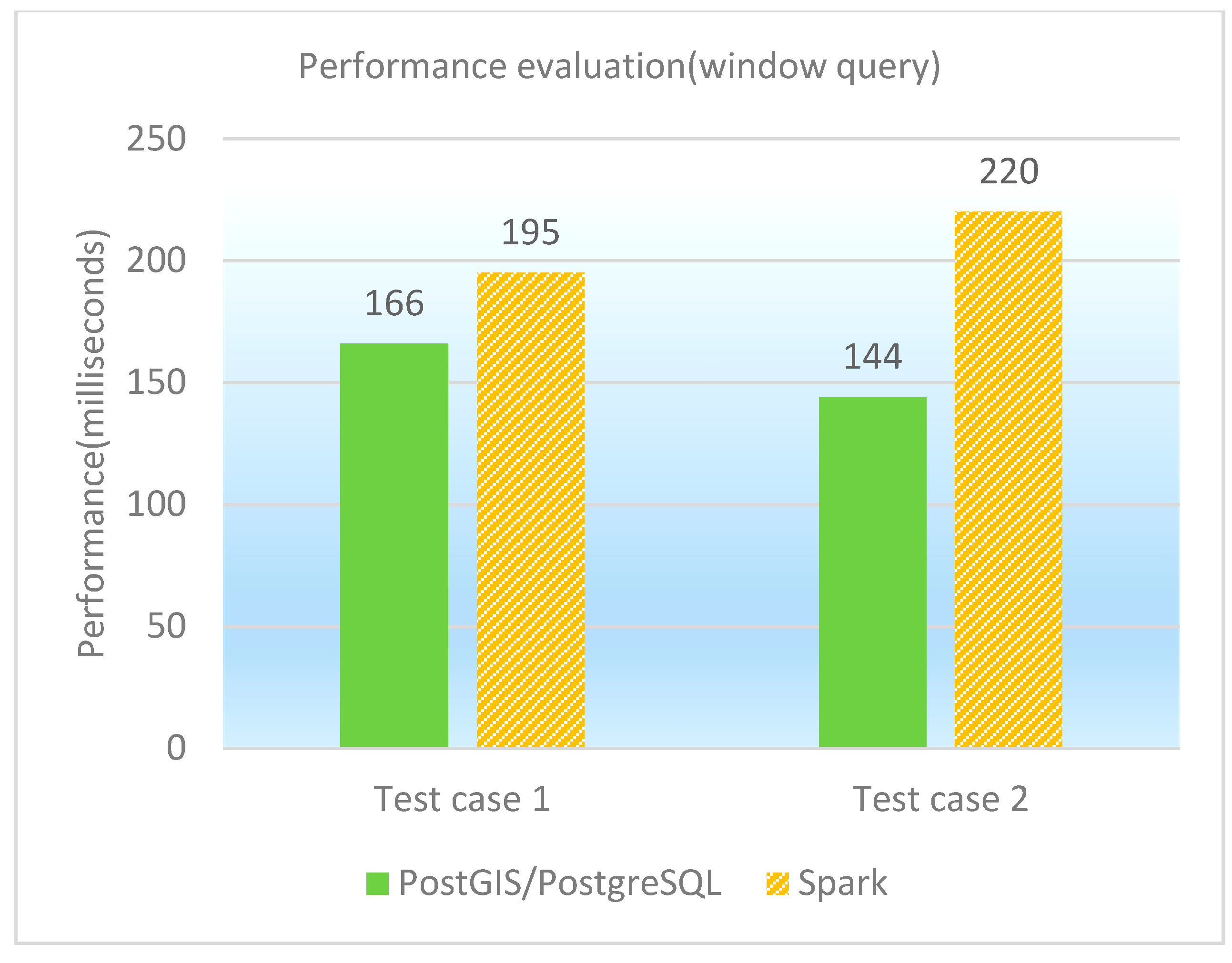
The window query is to find the spatial features that locate in a given rectangle. Two test cases as window queries are designed and performed on PostGIS/PostgreSQL, GeoSpark SQL and ESRI Spatial Framework for Hadoop, respectively. The concrete test cases are shown in Table 10, and the performance of window queries under different database platforms is shown in both Table 11 and Figure 8. It is observed that PostGIS/PostgreSQL performs better than GeoSpark SQL in window queries. The reason is similar to former point queries. When the query’s selection rate is very high, the spatial index plays a vital role and parallelization can only bring the cost of additional network transmission and scheduling, so that GeoSpark SQL is not as good as PostGIS/PostgreSQL in the two test cases.
6.3.5. Range Query
The range query is to find the spatial features that locate in a given polygon range. Two test cases as range queries are designed and performed on PostGIS/PostgreSQL, GeoSpark SQL and ESRI Spatial Framework for Hadoop, respectively. The concrete test cases are shown in Table 12, and the performance of range queries under different database platforms is shown in both Table 13 and Figure 9. It is observed that GeoSpark SQL and PostGIS/PostgreSQL are generally close in range query performance. The computational complexity of test case 1 that queries the polygon-type table is higher than that of test case 2, which queries the point-type table. As for test case 1, GeoSpark SQL performs better; while as for test case 2, PostGIS/PostgreSQL performs better. This also means that GeoSpark SQL is more sensitive to compute-intensive spatial queries. In addition, we notice that Spark is not a panacea. The traditional spatial database performs better than GeoSpark SQL in some scenarios, especially for the spatial queries with high selectivity.
6.3.6. Directional Query
The directional query is to find the spatial features that are on top of/under/on the left side of/on the right side of a given feature. Two test cases as directional queries are designed and performed on PostGIS/PostgreSQL, GeoSpark SQL and ESRI Spatial Framework for Hadoop, respectively. The concrete test cases are shown in Table 14, and the performance of directional queries under different database platforms is shown in both Table 15 and Figure 10. It is observed that PostGIS/PostgreSQL performs better than GeoSpark SQL in directional queries. The reason is similar to former point and window queries.
6.3.7. Topological Query
The topological query is to find the spatial features that have a specific topological relationship with the given feature. Two test cases as topological queries are designed and performed on PostGIS/PostgreSQL, GeoSpark SQL and ESRI Spatial Framework for Hadoop, respectively. The concrete test cases are illustrated in Table 16, and the performance of topological queries under different database platforms is shown in both Table 17 and Figure 11. It is observed that GeoSpark SQL performs much better than PostGIS/PostgreSQL in the test cases. Because the topological query is compute-intensive and more suitable for parallelization, GeoSpark SQL achieves an outstanding performance. However, PostGIS/PostgreSQL cannot take full advantage of the spatial index when dealing with the ‘Disjoint’ type testing queries, so there is a significant reduction in query efficiency.
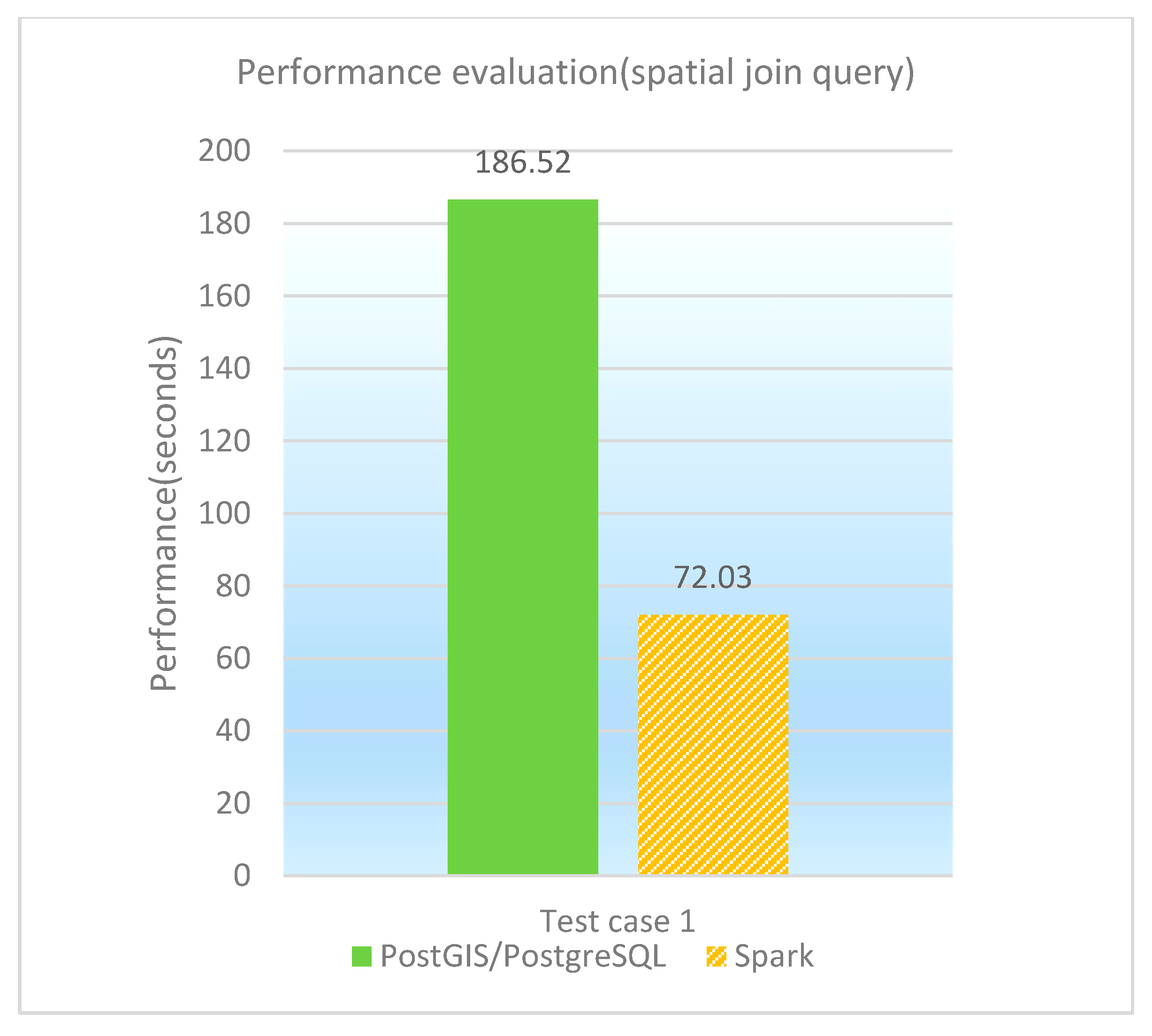
6.3.8. Spatial Join Query
The spatial join query involves with multi-tables, and is the most time-consuming for all spatial queries. A testing query is designed and performed on PostGIS/PostgreSQL and GeoSpark SQL, respectively. ESRI Spatial Framework for Hadoop does not support non-equivalent JOIN statements, so spatial join queries cannot be executed on that platform. The concrete test case is shown in Table 18, and the performance of spatial join queries under different database platforms is illustrated in both Table 19 and Figure 12. It is observed that GeoSpark SQL performs much better than PostGIS/PostgreSQL in the spatial join query, which benefits from Spark’s high performance computing advantages.
6.4. Discussion of Experimental Results
As for single-table queries, ESRI Spatial Framework for Hadoop performs stably but more time-consuming (the average query response time is about 50 s). Hadoop is a traditional MapReduce framework, but also with the distributed file system HDFS. In the Map query stage, the spatial data are read from the HDFS and processed in memory, and then all temporary results need to be written back to HDFS before initializing the Reduce stage. Hence, the efficiency of the ESRI Spatial Framework for Hadoop is relatively low. However, the results are stored in persistent storage, so the data are less likely to be lost, which means ESRI Spatial Framework for Hadoop is more suitable for offline batch processing of massive spatial data.
Due to the establishment of spatial index, the PostGIS/PostgreSQL’s average response time for simple conditional queries is 100 to 300 milliseconds or so. Hence, the query performance of PostGIS/PostgreSQL is more excellent than ESRI Spatial Framework for Hadoop. However, as for the kNN query and the spatial join query, it is much slower because the kNN query requires a full table scan before sorting and the spatial join query needs to perform the Cartesian product operation before spatial topological calculation, which is quite resource intensive. Especially for the disjoint query, a specific type of spatial join queries, it is difficult to use optimization strategies. Usually the whole spatial table needs to be scanned, so the spatial index cannot play a role, and thus leading to inefficiency.
Except for spatial join queries, GeoSpark SQL costs 200 milliseconds or so in other spatial queries, including the kNN query, which is proved to be inefficient in PostGIS/PostgreSQL. Moreover, compared with PostGIS/PostgreSQL, GeoSpark SQL achieves a 2.6× speedup in the spatial join query. On the one hand, it is due to Spark’s memory computing characteristics; on the other hand, the Spark framework also provides parallel processing capabilities. These make GeoSpark SQL particularly effective for query processing of massive spatial datasets. As a result, GeoSpark SQL performs better when dealing with compute-intensive spatial queries such as the kNN query and the spatial join query. However, we also notice that Spark is not a panacea. It is observed that the traditional spatial database performs better than GeoSpark SQL in some query scenarios, especially for the spatial queries with high selectivity such as the point query and the window query, which consume fewer disk I/O and computing resources than compute-intensive spatial queries.
7. Conclusions and Future Work
In order to address the increasingly large-scale spatial query processing requirement in the era of big data, we propose an effective framework GeoSpark SQL, which enables spatial queries on Spark. On the one hand, GeoSpark SQL provides a convenient SQL interface; on the other hand, GeoSpark SQL achieves both efficient storage management and high-performance parallel computing through integrating Hive and Spark. In this study, the following key issues are discussed and addressed: storage management methods under the GeoSpark SQL framework, the spatial query operator implementation approach in the Spark environment, and spatial query optimization methods under Spark. Experiments show that GeoSpark SQL is able to achieve real-time spatial query processing, with better performance especially when dealing with complex spatial queries such as kNN queries and spatial join queries.
(1) GeoSpark SQL can be seen as the elementary form of the future spatial database. Compared with the traditional spatial database, GeoSpark SQL is able to meet the changing requirements at a more agile speed, and has stronger robustness and the fault tolerance support. There are following advantages through integrating Spark as well as Hive into a spatial database framework: the Spark based spatial database can be extended horizontally. In order to deal with the increasing amount of spatial data, it can speed up spatial query processing through increasing the number of backend servers. Spark’s memory-based parallel computing advantage plays a more significant role in managing massive spatial data sets. At the same time, the expansion operation of clusters is transparent for users. However, as for the traditional spatial database deployed on a single host, only a limited number of concurrent spatial queries can be handled, and the query response is slower when managing massive spatial data. In addition, the establishment and update efficiency of the spatial index will gradually become unacceptable with the increasing amount of spatial data.
(2) The Spark based spatial database is more robust. Whether Spark is deployed on YARN, independent scheduler or other resource scheduling systems, ZooKeeper election is used to avoid the master node failure. At the same time, even if the slave node fails, Spark will automatically re-read the replica data based on the metadata that contains data distribution information. Hence, the Spark based spatial database is able to continuously provide query services as long as more than half of the nodes are alive in the cluster. However, the traditional spatial database like PostGIS/PostgreSQL can ensure service only by the master/slave mode. Once the master mode fails, it will take some time to switch to the slave node. However, it also means that the database service has the risk of being stopped. Moreover, the migration process and other configurations require manual prior definition, which is time consuming and cannot achieve adaptive selection like Spark.
(3) The Spark based spatial database is able to support new features and requirements with better efficiency. In the Spark system, spatial operators can be customized through extending UDFs, utilizing Java to write functions that can be directly used in the program. As for the traditional database, before extending UDFs there is a need to learn a lot of knowledge to understand the backend implementation architecture of the database, and the development efficiency is much lower than Spark. In addition, due to the advantages of high-performance cluster computing, the Spark based spatial database has better performance than the traditional database, especially for complex applications that contain extensive read/write tasks or iterations (such as kNN classification).
(4) The Spark based spatial database is user-friendlier. To deploy GeoSpark SQL, it only requires adding java package dependencies in Spark and starting Spark SQL terminal, and then users can submit spatial queries. Without using Spark Scala scripts, spatial queries can be simply formed by SQL statements with spatial UDFs in GeoSpark SQL. Since SQL is simple and has been wildly used, it is more convenient to use GeoSpark SQL than other Spark-based spatial query systems.
In the future, we plan to improve GeoSpark SQL’s design and implementation approaches from the following aspects: on the one hand, we hope to explore a more complex spatial index to further optimize spatial query processing in the Spark/Hive environment (e.g., improving the performance of window queries); on the other hand, more servers and larger-volume spatial data (e.g., road network datasets) are expected to be deployed to build up a more complex test environment to validate and improve system performance.
Acknowledgments
This research was supported by grants from the National Key Research and Development Program of China (2017YFB0503602), the National Natural Science Foundation of China (41401449, 41501162, 41771425), the Scientific Research Key Program of Beijing Municipal Commission of Education (KM201611417004), the Beijing Philosophy and Social Science Foundation, the Talent Optimization Program of Beijing Union University and State Key Laboratory of Resources and Environmental Information System.
Author Contributions
Zhou Huang and Xia Peng conceived and designed the experiments; Yiran Chen performed the experiments; Lin Wan and Xia Peng analyzed the data; Zhou Huang and Yiran Chen wrote the paper.
Conflicts of Interest
The authors declare no conflict of interest.
References
- Zhong, Y.; Han, J.; Zhang, T.; Li, Z.; Fang, J.; Chen, G. Towards parallel spatial query processing for big spatial data. In Proceedings of the 2012 IEEE 26th International Parallel and Distributed Processing Symposium Workshops & PhD Forum (IPDPSW), Shanghai, China, 21–25 May 2012; pp. 2085–2094. [Google Scholar]
- Moniruzzaman, A. Newsql: Towards next-generation scalable rdbms for online transaction processing (oltp) for big data management. Int. J. Database Theory Appl. 2014, 7, 121–130. [Google Scholar] [CrossRef]
- Chen, C.; Lin, J.; Wu, X.; Wu, J.; Lian, H. Massive geospatial data cloud storage and services based on nosql database technique. J. Geo-Inf. Sci. 2013, 15, 166–174. [Google Scholar] [CrossRef]
- Liu, Y.; Jing, N.; Chen, L.; Wei, X. Algorithm for processing k-nearest join based on r-tree in mapreduce. J. Softw. 2013, 24, 1836–1851. [Google Scholar] [CrossRef]
- GIS Tools for Hadoop. Available online: http://esri.github.io/gis-tools-for-hadoop/ (accessed on 14 July 2017).
- Spatialhadoop. Available online: http://spatialhadoop.cs.umn.edu/ (accessed on 14 July 2017).
- Hadoop-GIS. Available online: http://bmidb.cs.stonybrook.edu/hadoopgis/index (accessed on 14 July 2017).
- Tripathy, A.; Mishra, L.; Patra, P.K. An efficient approach for distributed spatial query optimization using filters. In Proceedings of the 2010 3rd International Conference on Advanced Computer Theory and Engineering (ICACTE), Chengdu, China, 20–22 August 2010. [Google Scholar]
- Cary, A.; Sun, Z.; Hristidis, V.; Rishe, N. Experiences on processing spatial data with mapreduce. In Proceedings of the International Conference on Scientific and Statistical Database Management, New Orleans, LA, USA, 2–4 June 2009; pp. 302–319. [Google Scholar]
- Wang, Y.; Wang, S. Research and implementation on spatial data storage and operation based on hadoop platform. In Proceedings of the 2010 Second IITA International Conference on Geoscience and Remote Sensing (IITA-GRS), Qingdao, China, 28–31 Augsut 2010. [Google Scholar]
- Yan, B.; Rhodes, P.J. IDEA—An API for parallel computing with large spatial datasets. In Proceedings of the 2011 International Conference on Parallel Processing (ICPP), Taipei, Taiwan, 13–16 September 2011; pp. 355–364. [Google Scholar]
- Wan, L.; Huang, Z.; Peng, X. An Effective NoSQL-Based Vector Map Tile Management Approach. ISPRS Int. J. Geo-Inf. 2016, 5, 215. [Google Scholar] [CrossRef]
- Cui, X. Distributed Storage Management and Parallel Processing Technologies of Massive Spatial Data. Master’s Thesis, National University of Defense Technology, Changsha, China, 2010. [Google Scholar]
- Zhong, Y.; Zhu, X.; Cheng, Z.; Liao, H.; Fang, J. A high efficiency management method for massive spatial data based on the distributed storage computing architecture. In Proceedings of the China National Conference on High Performance Computing, Beijing, China, 26 October 2011. [Google Scholar]
- HadoopDB. Available online: http://db.cs.yale.edu/hadoopdb/hadoopdb.html (accessed on 14 July 2017).
- Apache Spark. Available online: http://spark.apache.org/docs/latest/ (accessed on 14 July 2017).
- Understanding Spark’s Core RDD. Available online: http://www.infoq.com/cn/articles/spark-core-rdd/ (accessed on 14 July 2017).
- Xie, X.; Xiong, Z.; Hu, X.; Zhou, G.; Ni, J. On massive spatial data retrieval based on spark. In Proceedings of the International Conference on Web-Age Information Management, Macau, China, 16–18 June 2014; pp. 200–208. [Google Scholar]
- Wen, X.; Luo, K.; Chen, R. A framework of distributed spatial data analysis based on shark/spark. J. Geo-Inf. Sci. 2015, 17, 401–407. [Google Scholar] [CrossRef]
- You, S.; Zhang, J.; Gruenwald, L. Large-scale spatial join query processing in cloud. In Proceedings of the 2015 31st IEEE International Conference on Data Engineering Workshops (ICDEW), Seoul, Korea, 13–17 April 2015; pp. 34–41. [Google Scholar]
- Yu, J.; Wu, J.; Sarwat, M. Geospark: A cluster computing framework for processing large-scale spatial data. In Proceedings of the the 23rd SIGSPATIAL International Conference on Advances in Geographic Information Systems, Bellevue, WA, USA, 3–6 November 2015. [Google Scholar]
- Baig, F.; Mehrotra, M.; Vo, H.; Wang, F.; Saltz, J.; Kurc, T. Sparkgis: Efficient comparison and evaluation of algorithm results in tissue image analysis studies. In Proceedings of the Biomedical Data Management and Graph Online Querying: VLDB 2015 Workshops, Big-O (Q) and DMAH, Waikoloa, HI, USA, 31 August–4 September 2015. [Google Scholar]
- Galić, Z. Spatio-temporal data streams and big data paradigm. In Spatio-Temporal Data Streams; Springer: New York, NY, USA, 2016; pp. 47–69. ISBN 978-1-4939-6575-5. [Google Scholar]
- Kini, A.; Emanuele, R. Geotrellis: Adding Geospatial Capabilities to Spark, Spark Summit 2014. Available online: https://spark-summit.org/2014/geotrellis-adding-geospatial-capabilities-to-spark/ (accessed on 14 July 2017).
- Tang, M.; Yu, Y.; Malluhi, Q.M.; Ouzzani, M.; Aref, W.G. Locationspark: A distributed in-memory data management system for big spatial data. Proc. VLDB Endow. 2016, 9, 1565–1568. [Google Scholar] [CrossRef]
- Zhang, F.; Zhou, J.; Liu, R.; Du, Z.; Ye, X. A New Design of High-Performance Large-Scale GIS Computing at a Finer Spatial Granularity: A Case Study of Spatial Join with Spark for Sustainability. Sustainability 2016, 8, 926. [Google Scholar] [CrossRef]
- Du, Z.; Zhao, X.; Ye, X.; Zhou, J.; Zhang, F.; Liu, R. An Effective High-Performance Multiway Spatial Join Algorithm with Spark. ISPRS Int. J. Geo-Inf. 2017, 6, 96. [Google Scholar] [CrossRef]
- Zaharia, M.; Chowdhury, M.; Franklin, M.J.; Shenker, S.; Stoica, I. Spark: Cluster computing with working sets. In Proceedings of the Usenix Conference on Hot Topics in Cloud Computing, Boston, MA, USA, 22–25 June 2010; p. 10. [Google Scholar]
- Apache Drill. Available online: http://drill.apache.org/ (accessed on 14 July 2017).
- Apache Impala. Available online: http://impala.apache.org/ (accessed on 14 July 2017).
- Shark, Spark SQL, Hive on Spark, and the Future of SQL on Apache Spark. Available online: https://databricks.com/blog/2014/07/01/shark-spark-sql-hive-on-spark-and-the-future-of-sql-on-spark.html (accessed on 14 July 2017).
- Introduction to Spark SQL. Available online: http://www.cnblogs.com/shishanyuan/p/4723604.html (accessed on 14 July 2017).
- International Organization for Standardization. Information Technology—Database Languages—SQL Multimedia and Application Packages—Part 3: Spatial; ISO/IEC 13249-3:2016; International Organization for Standardization: Geneva, Switzerland, 2016. [Google Scholar]
Figure 1.
Running framework of Spark SQL.

Figure 2.
GeoSpark SQL framework.
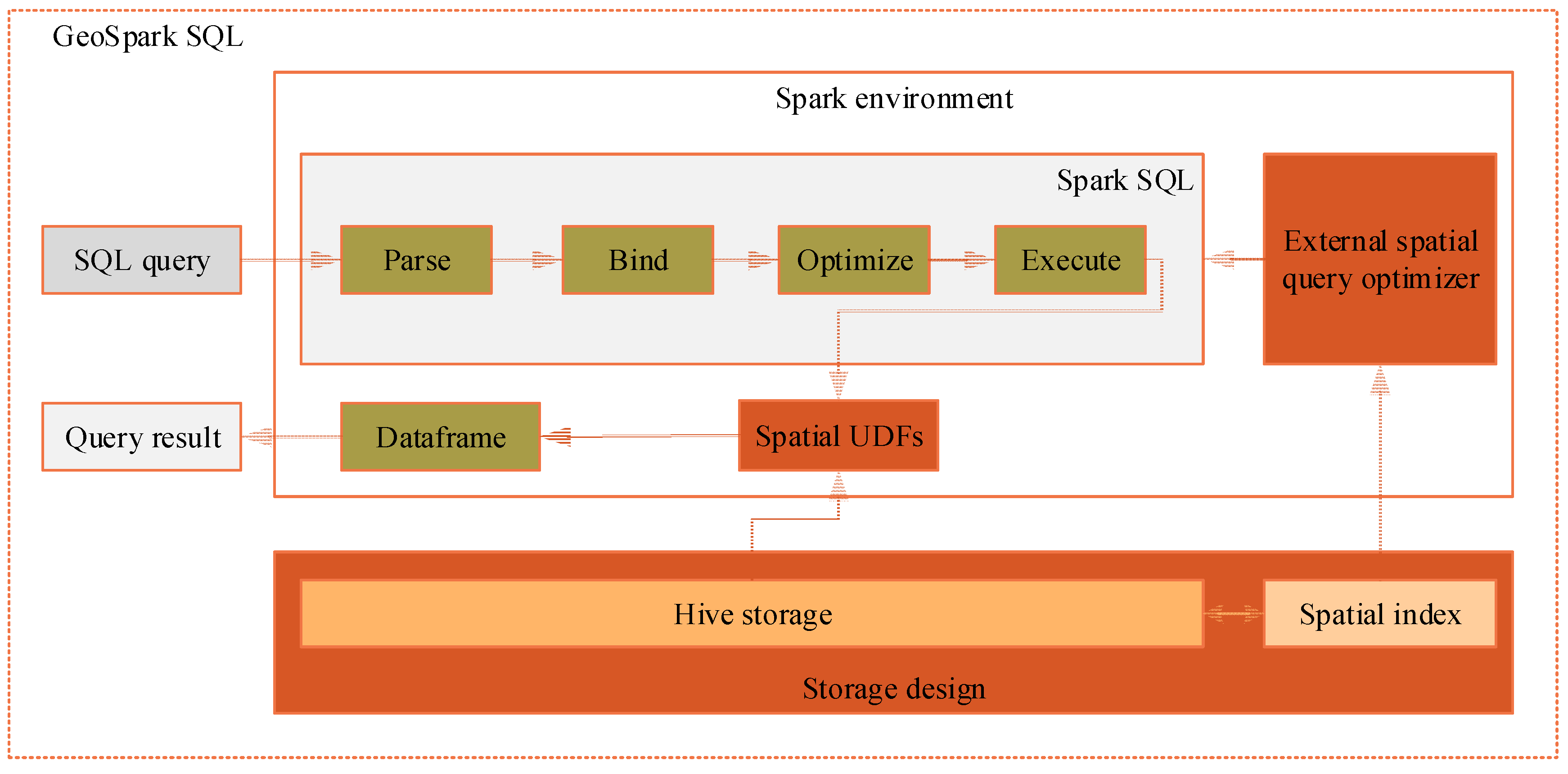
Figure 3.
Simulated point dataset of northwest pacific typhoon routes for 5000 years.

Figure 4.
Land use dataset of Zhenlong Town.

Figure 5.
Performance comparison graph of attribute queries (in milliseconds).

Figure 6.
Performance comparison graph of kNN queries (in milliseconds).
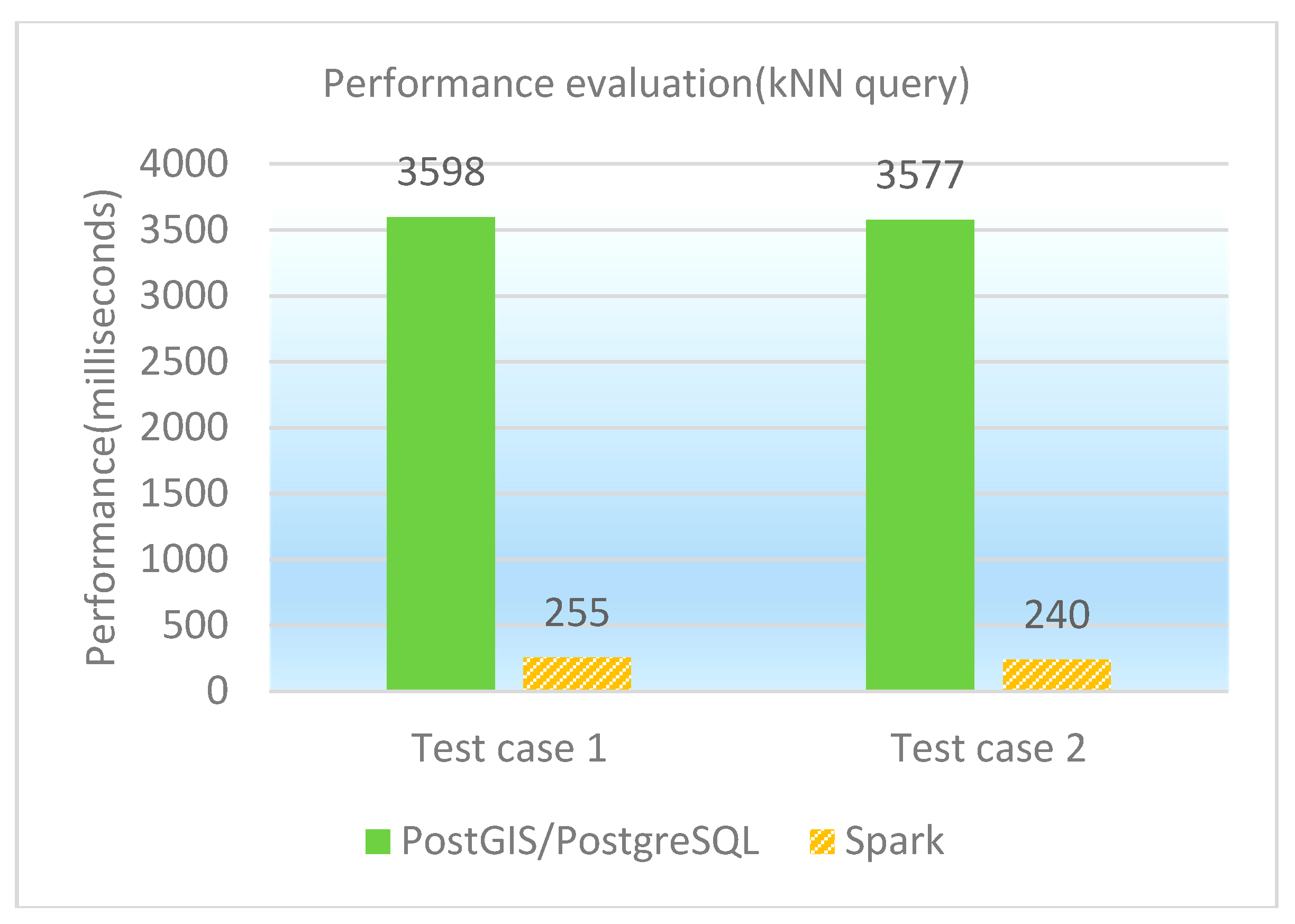
Figure 7.
Performance comparison graph of point queries (in milliseconds).

Figure 8.
Performance comparison graph of window queries (in milliseconds).

Figure 9.
Performance comparison graph of range queries (in milliseconds).
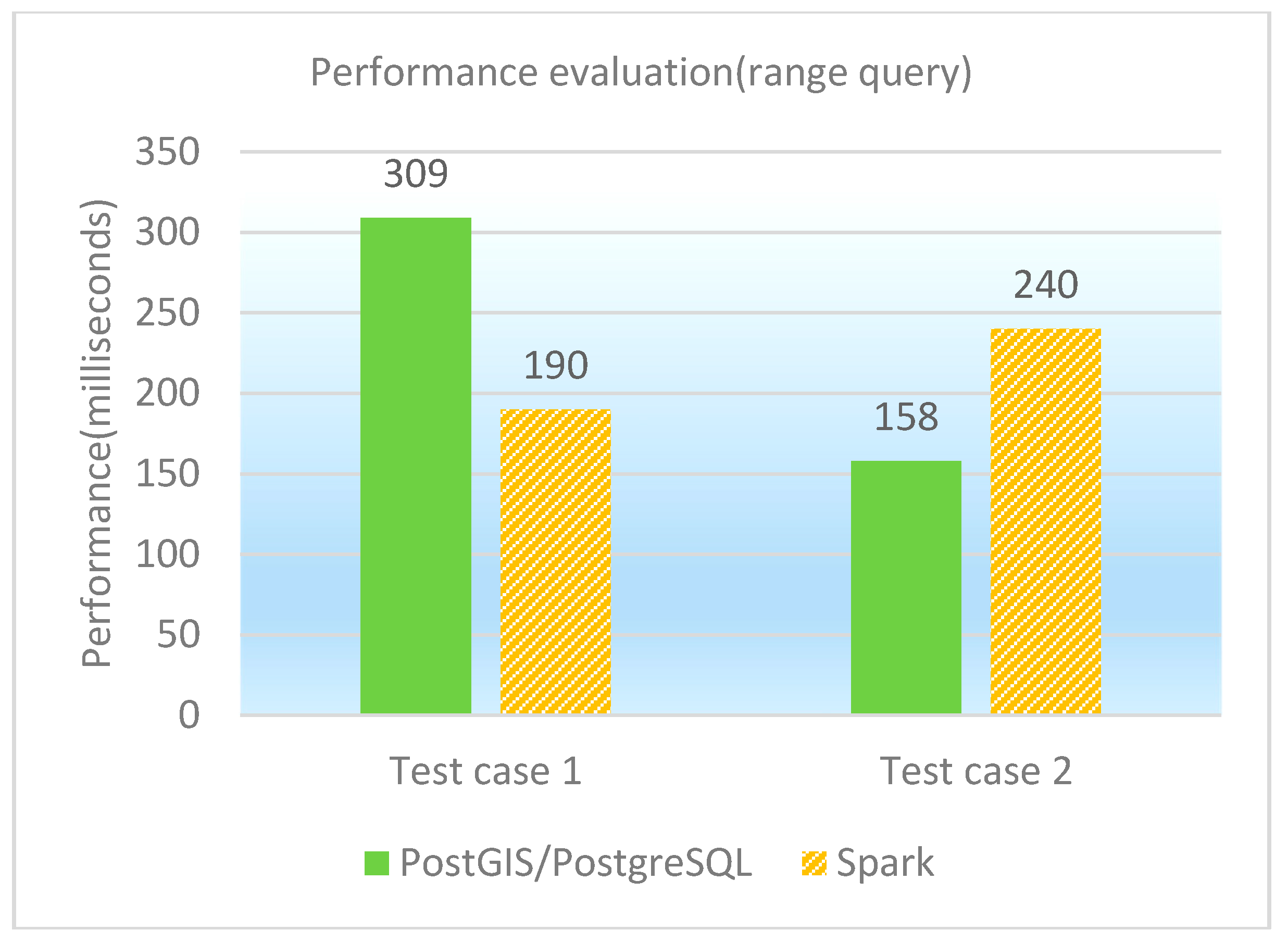
Figure 10.
Performance comparison graph of directional queries (in milliseconds).
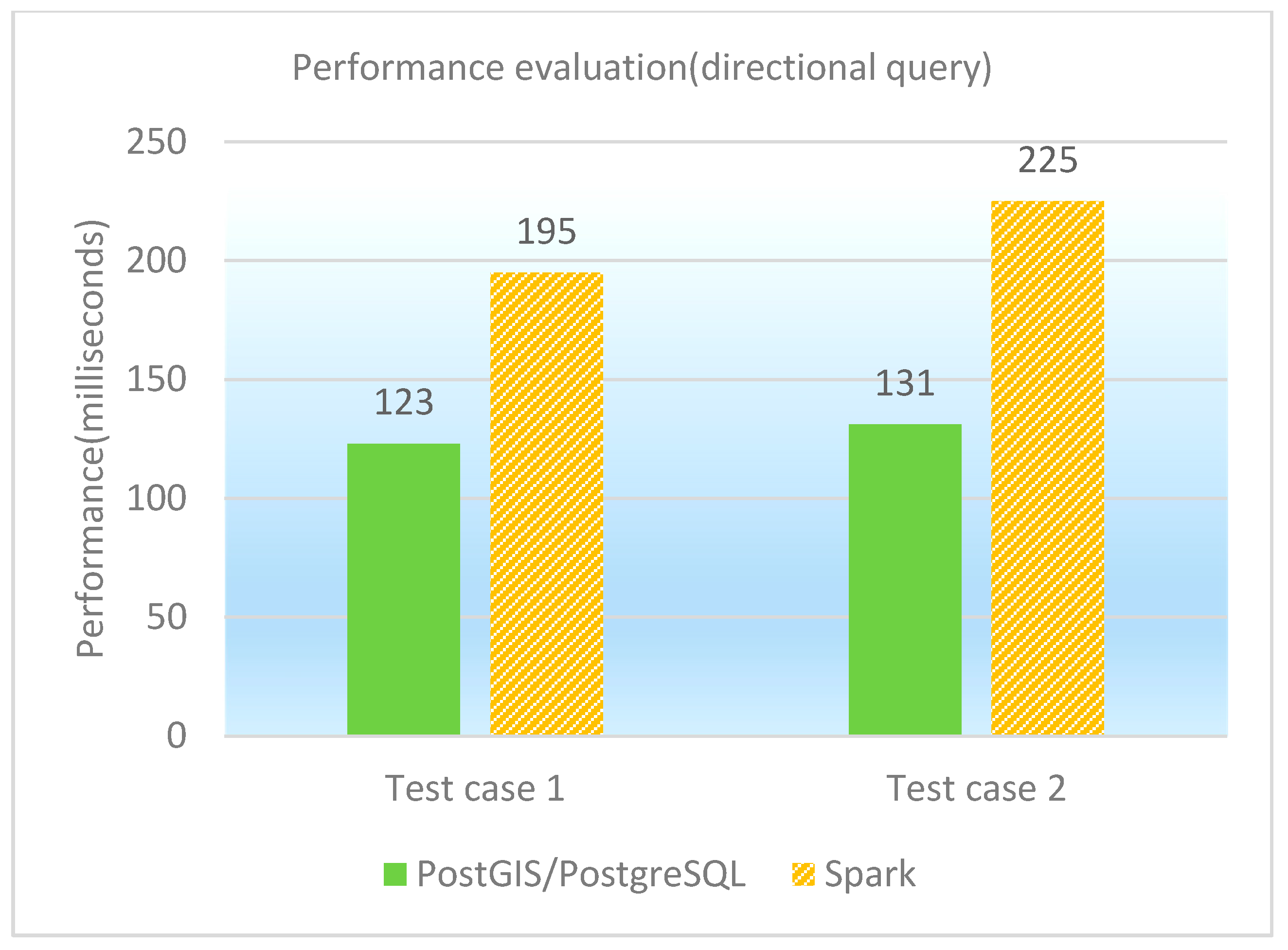
Figure 11.
Performance comparison graph of topological queries (in milliseconds).
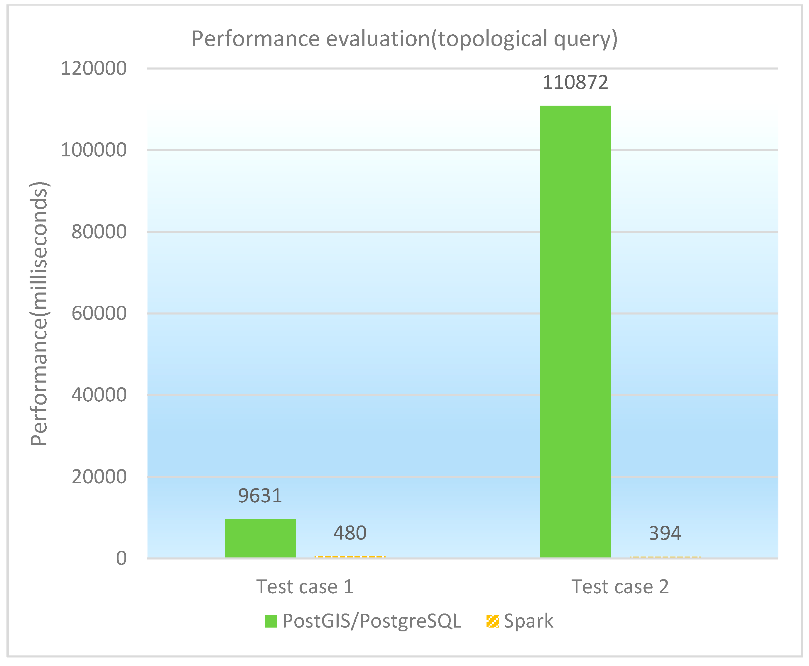
Figure 12.
Performance comparison graph of spatial join queries (in seconds).

Table 1.
Descriptions of extended spatial UDFs in Spark.
| Function Name | Function Description |
|---|---|
| ST_Equals | If the two features are identical, return true; otherwise return false. |
| ST_Disjoint | If neither the two features’ boundaries intersect, nor the two elements intersect inside, return true; otherwise return false. |
| ST_Touches | If the two features’ boundaries intersect, return true; otherwise return false. |
| ST_Within | If the interior of a given feature does not intersect the outside of another feature, return true; otherwise return false. |
| ST_Overlaps | If the two features intersect inside, return true; otherwise return false. |
| ST_Crosses | If the line-type feature intersects the interior of the polygon-type feature, return true; otherwise return false. |
| ST_Intersects | If the two features intersect, return true; otherwise return false. |
| ST_Contains | If the given feature contains the other feature, return true; otherwise return false. |
| ST_Relate | The inputs are two features and a string describing the 9-Intersection Model (such as “T********”), and the output is a ‘Boolean’ value. If the two features satisfy the given 9-Intersection model, return true; otherwise return false. |
Table 2.
Descriptions of testing platforms.
| Software Platform for Testing | PostGIS/PostgreSQL | GeoSpark SQL and ESRI Spatial Framework for Hadoop |
|---|---|---|
| Overview | PostGIS/PostgreSQL runs on a single server. | These two systems run on a computing cluster hosted on Meituan Cloud. There are five compute nodes. One is the master node and the others are slave nodes. Moreover, the nodes are connected by a 10-gigabit network. |
| Hardware configuration | CPU: Intel i7-4770 3.4 GHz | CPU: 4 cores |
| RAM: 8 GB | RAM: 8 GB | |
| Hard disk: 1 TB 7200 rpm | Hard disk:400 GB | |
| Software configuration | PostgreSQL version: 8.4 PostGIS version: 8.1 | JDK (Java Development Kit) version: 7u79 Hadoop version: 2.4.1 Hive version: 1.0.1 Spark version: 1.4.1 |
Table 3.
Descriptions of test datasets.
| Description | Point-Type Dataset | Polygon-Type Dataset |
|---|---|---|
| Overview | A simulated point dataset of northwest pacific typhoon routes for 5000 years | A land use dataset of Zhenlong Town, Heng County, Nanning City, Guangxi Province of China |
| Table name | cyclonepoint | zhenlongxiang |
| Size of shape file | 929 MB | 723 MB |
| Number of features | 4,971,784 points | 128,888 polygons |
Table 4.
Test cases of attribute queries.
| No. | Test Case | Number of Results |
|---|---|---|
| 1 | SELECT * FROM cyclonepoint WHERE UTC_Yr = 180 AND UTC_Mon = 9 AND UTC_Day = 2 AND UTC_Hr = 12 | 9 rows |
| 2 | SELECT * FROM cyclonepoint WHERE pres < 860 | 4576 rows |
| 3 | SELECT * FROM zhenlongxiang WHERE LUCODE = ‘205’ | 1522 rows |
| 4 | SELECT * FROM zhenlongxiang WHERE LUCODE = ‘102’ | 476 rows |
Table 5.
Performance of attribute queries (in milliseconds).
| No. | PostGIS/PostgreSQL | GeoSpark SQL | ESRI Spatial Framework for Hadoop |
|---|---|---|---|
| 1 | 660 | 170 | 40,263 |
| 2 | 848 | 230 | 39,904 |
| 3 | 1265 | 215 | 61,473 |
| 4 | 1190 | 185 | 64,664 |
Table 6.
Test cases of kNN queries.
| No. | Test Case | Number of Results |
|---|---|---|
| 1 | SELECT * FROM cyclonepoint ORDER BY ST_Distance(geom, ST_GeomFromText(‘POINT(120 40)’,4326)) LIMIT 50 | 50 rows |
| 2 | SELECT * FROM cyclonepoint ORDER BY ST_Distance(geom, ST_GeomFromText(‘POINT(130 40)’,4326)) LIMIT 100 | 100 rows |
Table 7.
Performance of kNN queries (in milliseconds).
| No. | PostGIS/PostgreSQL | GeoSpark SQL | ESRI Spatial Framework for Hadoop |
|---|---|---|---|
| 1 | 3598 | 255 | 51,025 |
| 2 | 3577 | 240 | 52,074 |
Table 8.
Test cases of point queries.
| No. | Test Case | Number of Results |
|---|---|---|
| 1 | SELECT * FROM zhenlongxiang WHERE ST_Within(ST_GeomFromText(‘POINT(600000 2522000)’), geom) | 1 row |
| 2 | SELECT * FROM zhenlongxiang WHERE ST_Within(ST_GeomFromText(‘POINT(590000 2522000)’), geom) | 1 row |
Table 9.
Performance of point queries (in milliseconds).
| No. | PostGIS/PostgreSQL | GeoSpark SQL | ESRI Spatial Framework for Hadoop |
|---|---|---|---|
| 1 | 103 | 195 | 66,508 |
| 2 | 98 | 220 | 66,360 |
Table 10.
Test cases of window queries.
| No. | Test Case | Number of Results |
|---|---|---|
| 1 | SELECT * FROM zhenlongxiang WHERE ST_Intersects(geom, ST_GeomFromText(‘POLYGON((617000 2520000,619000 2520000,619000 2522000,617000 2522000,617000 2520000))’)) | 162 rows |
| 2 | SELECT * FROM cyclonepoint WHERE ST_Intersects(geom, ST_GeomFromText(‘POLYGON((110 10,111 10,111 11,110 11,110 10))’,4326)) | 1938 rows |
Table 11.
Performance of window queries (in milliseconds).
| No. | PostGIS/PostgreSQL | GeoSpark SQL | ESRI Spatial Framework for Hadoop |
|---|---|---|---|
| 1 | 166 | 195 | 66,318 |
| 2 | 114 | 220 | 42,662 |
Table 12.
Test cases of range queries.
| No. | Test Case | Number of Results |
|---|---|---|
| 1 | SELECT * FROM zhenlongxiang WHERE ST_Intersects(geom, ST_GeomFromText(‘POLYGON((617000 2520000,620000 2520000,619000 2522000,616000 2522000,617000 2520000))’)) | 338 rows |
| 2 | SELECT * FROM cyclonepoint WHERE ST_Intersects(geom, ST_GeomFromText(‘POLYGON((120 10,121 10.55,122 11,121 10.3,120 10))’,4326)) | 3191 rows |
Table 13.
Performance of range queries (in milliseconds).
| No. | PostGIS/PostgreSQL | GeoSpark SQL | ESRI Spatial Framework for Hadoop |
|---|---|---|---|
| 1 | 309 | 190 | 63,220 |
| 2 | 158 | 240 | 41,691 |
Table 14.
Test cases of directional queries.
| No. | Test Case | Number of Results |
|---|---|---|
| 1 | SELECT * FROM cyclonepoint WHERE geom &<| ST_GeomFromText(‘POINT(90 2.5)’, 4326) AND geom |&> ST_GeomFromText(‘POINT(90 2)’, 4326) | 690 rows |
| 2 | SELECT * FROM zhenlongxiang WHERE geom |&> ST_GeomFromText(‘POINT(590000 2555000)’) | 223 rows |
Table 15.
Performance of directional queries (in milliseconds).
| No. | PostGIS/PostgreSQL | GeoSpark SQL | ESRI Spatial Framework for Hadoop |
|---|---|---|---|
| 1 | 123 | 195 | 42,623 |
| 2 | 131 | 225 | 62,483 |
Table 16.
Test cases of topological queries.
| No. | Test Case | Number of Results |
|---|---|---|
| 1 | SELECT IDCODE FROM zhenlongxiang WHERE ST_Disjoint(geom,ST_GeomFromText(‘POLYGON((517000 1520000,619000 1520000,619000 2530000,517000 2530000,517000 1520000))’)); | 85,236 rows |
| 2 | SELECT fid FROM cyclonepoint WHERE ST_Disjoint(geom,ST_GeomFromText(‘POLYGON((90 3,170 3,170 55,90 55,90 3))’,4326)) | 60,591 rows |
Table 17.
Performance of topological queries (in milliseconds).
| No. | PostGIS/PostgreSQL | GeoSpark SQL | ESRI Spatial Framework for Hadoop |
|---|---|---|---|
| 1 | 9631 | 480 | 40,784 |
| 2 | 110872 | 394 | 64,217 |
Table 18.
Test cases of spatial join queries.
| No. | Test Case | Number of Results |
|---|---|---|
| 1 | SELECT DISTINCT c.IDCODE FROM | 1465 rows |
| (SELECT IDCODE, geom FROM zhenlongxiang WHERE LUCODE = ‘202’ OR LUCODE = ‘203’) c, | ||
| (SELECT geom FROM zhenlongxiang WHERE LUCODE = ‘114’ OR LUCODE = ‘205’ OR LUCODE = ‘113’ OR LUCODE = ‘111’) w, | ||
| (SELECT geom FROM zhenlongxiang WHERE LUCODE = ‘102’ OR LUCODE = ‘104’) r | ||
| WHERE ST_Touches(c.geom,r.geom) AND ST_Touches(c.geom,w.geom) |
Table 19.
Performance of spatial join queries (in seconds).
| No. | PostGIS/PostgreSQL | GeoSpark SQL |
|---|---|---|
| 1 | 186.52 | 72.03 |
© 2017 by the authors. Licensee MDPI, Basel, Switzerland. This article is an open access article distributed under the terms and conditions of the Creative Commons Attribution (CC BY) license (http://creativecommons.org/licenses/by/4.0/).
Share and Cite
MDPI and ACS Style
Huang, Z.; Chen, Y.; Wan, L.; Peng, X. GeoSpark SQL: An Effective Framework Enabling Spatial Queries on Spark. ISPRS Int. J. Geo-Inf. 2017, 6, 285. https://doi.org/10.3390/ijgi6090285
AMA Style
Huang Z, Chen Y, Wan L, Peng X. GeoSpark SQL: An Effective Framework Enabling Spatial Queries on Spark. ISPRS International Journal of Geo-Information. 2017; 6(9):285. https://doi.org/10.3390/ijgi6090285
Chicago/Turabian StyleHuang, Zhou, Yiran Chen, Lin Wan, and Xia Peng. 2017. "GeoSpark SQL: An Effective Framework Enabling Spatial Queries on Spark" ISPRS International Journal of Geo-Information 6, no. 9: 285. https://doi.org/10.3390/ijgi6090285
Note that from the first issue of 2016, this journal uses article numbers instead of page numbers. See further details here.