Multi-Temporal Sentinel-1 and -2 Data Fusion for Optical Image Simulation


RIKEN Center for Advanced Intelligence Project, RIKEN, Tokyo 103-0027, Japan
*
Authors to whom correspondence should be addressed.
ISPRS Int. J. Geo-Inf. 2018, 7(10), 389; https://doi.org/10.3390/ijgi7100389
Submission received: 26 July 2018
/
Revised: 8 September 2018
/
Accepted: 21 September 2018
/
Published: 26 September 2018
(This article belongs to the Special Issue Data Mining and Feature Extraction from Satellite Images and Point Cloud Data)
Abstract
:In this paper, we present the optical image simulation from synthetic aperture radar (SAR) data using deep learning based methods. Two models, i.e., optical image simulation directly from the SAR data and from multi-temporal SAR-optical data, are proposed to testify the possibilities. The deep learning based methods that we chose to achieve the models are a convolutional neural network (CNN) with a residual architecture and a conditional generative adversarial network (cGAN). We validate our models using the Sentinel-1 and -2 datasets. The experiments demonstrate that the model with multi-temporal SAR-optical data can successfully simulate the optical image; meanwhile, the state-of-the-art model with simple SAR data as input failed. The optical image simulation results indicate the possibility of SAR-optical information blending for the subsequent applications such as large-scale cloud removal, and optical data temporal super-resolution. We also investigate the sensitivity of the proposed models against the training samples, and reveal possible future directions.
1. Introduction
The optical data provided by Sentinel-2 has 13 spectral bands from visible, near infrared to short wave infrared spectrum, with a 5-day revisit time at the equator [1]. Sentinel-2 is useful in time-series analysis such as land cover changes and damage area detection. Change analysis using optical data assumes that all investigated images are cloud-free to classify every pixel in the image, which is often not possible, especially for the cloudy areas of the earth. Usually, there is only one low-cloudy image nearly every month in the cloudy area. Some researchers have reportedly used data from alternative months (previous or next) to composite the data corrupted by clouds [2,3]. However, these methods remove only small clouds and also ignore the changes between monthly data. All above limitations significantly influence the temporal resolution of optical datasets, and the subsequent time-series analysis. In order to increase the temporal resolution, it is necessary to combine other remote sensing data resources, and conduct multi-source data fusion to predict clean Sentinel-2 images.
The last few decades have witnessed a rapid growth in SAR data. SAR data captured by Sentinel-1 exhibits totally different characteristics from that of the optical data. Sentinel-1 has the ability to provide routine, day and night, all-weather resolution observation, and can also overcome various kinds of bad weather conditions such as clouds, rain, smoke and fog [4]. In particular, it is expected to provide near daily coverage over Europe and Canada [4]. Therefore, one obvious question arises: can we use SAR data to predict the optical image?
Recently, many researchers have contributed to the information fusion of SAR and optical images with different motives. Researchers [4] have adopted Intensity Hue Saturation (IHS) to integrate hyperspectral, and Topographic SAR into a single image to enhance urban surface features. Some groups [5] tried to remove speckle noise from SAR data via fusion of two data sources. Inspired by the image-to-image translation technique [6] in the field of computer vision (known as pix2pix), Merkle et al. generated SAR-like images based on deep learning to increase the number of precise ground control points for SAR and optical image matching [7]. The previous works conducted the fusion of SAR and optical data to produce an intermediate image [7] or final application results. Whether or not the SAR data can be directly translated to optical data remains a concern. Very recently, Wang et al. [8] tried to generate high quality visible images from SAR images using the convolutional neural network (CNN) based method. Merkle et al. [9] proposed to generate artificial optical images from SAR datasets via the pix2pix model. Following [9], Schmitt et al. further investigated the potential of the pix2pix model for the simulation of Sentinel-2 imagery from Sentinel-1 data [10]. Unfortunately, from the visual results presented in the reference [10], the generated optical images are far from the original images.
In this work, we aim to investigate the possibility of optical data simulation from SAR data. We have adopted deep learning based methods for the optical simulation for the following three reasons. First, a deep CNN can efficiently capture the image characteristics. Second, several smart techniques have been proposed for training CNN, such as batch normalization (BN) [11], residual networks (ResNets) [12] and Rectifier Linear Unit (ReLU) [13]. Recently, a generative adversarial network (GAN) has been proposed and demonstrated to be useful in data generation. Third, a deep architecture can be accelerated by a graphics processing unit (GPU).
We chose to use two methods: CNN with ResNets and cGAN [6] to complete the task. Equipped with state-of-the-art data simulation algorithms, we investigated the possibility of optical image simulation from single SAR imagery acquired at a similar period, and multi-temporal SAR-optical images (SAR imagery with the side information from previous or next time pairs of SAR and optical images). Our experiments on Sentinel-1 and -2 data demonstrate the necessity of using multi-temporal images as input and the effectiveness of cGAN.
Our method can be regarded as the extension of the pix2pix model adopted in the reference [10] with two advantages. Firstly, our model utilizes the ResNets, which have been proved to be more suitable for the image simulation task [14] compared to the Unet network adopted in the pix2pix model [6]. Secondly, we extend the input from SAR data only to the multi-temporal SAR-optical dataset, which will be justified to be very useful in the optical data simulation. Besides the temporal super-resolution of optical datasets, our model can also be extended to other applications, such as cross-domain remote sensing image classification [15] and retrieval [16].
2. Approaches
2.1. Problem Formulation
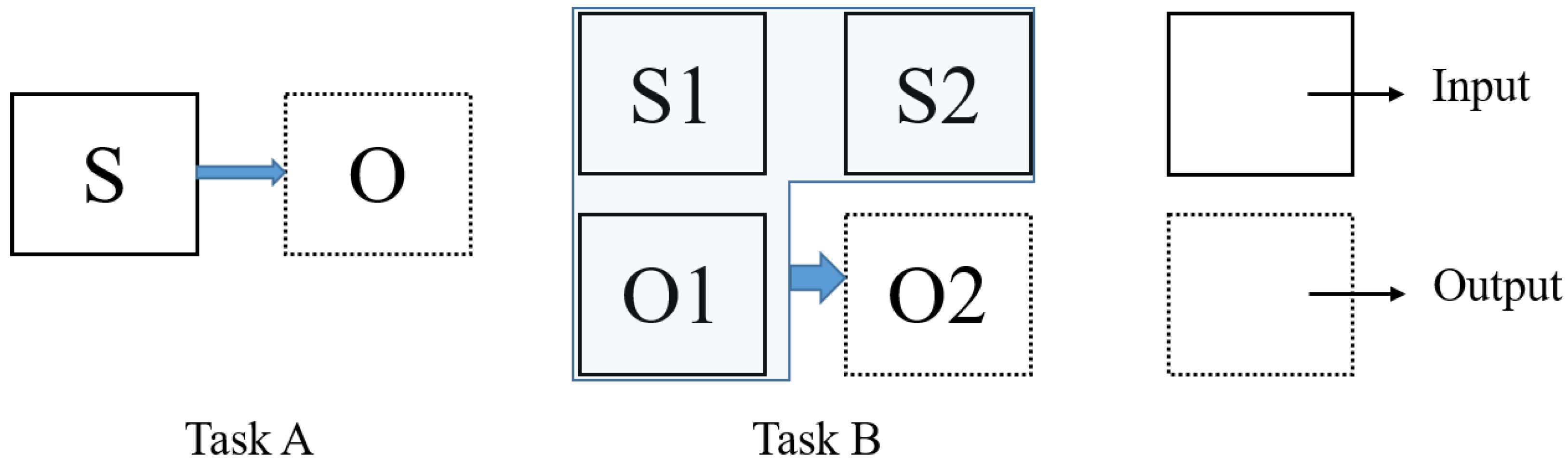
The purpose of this work is to simulate an optical image using either a single SAR image or multi-temporal SAR-optical images, which is outlined in Figure 1. The figure illustrates two tasks of optical image simulation. Task A shows the optical image simulation directly from the SAR data, and Task B displays the simulation from SAR (S2) combined with the additional information from the previous time pairs of SAR and optical data (S1 and O1). Task B is also referred to as multi-temporal fusion based optical image simulation. The CNN and cGAN are adopted to complete the simulation tasks, and the details of the investigated methods are presented in the subsequent section.
2.2. Architecture of CNN Network
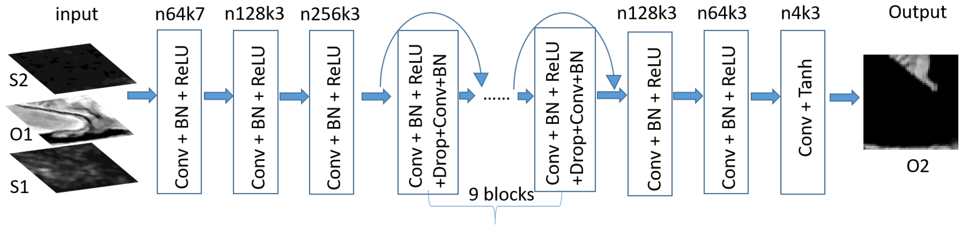
The CNN optical generation network is illustrated in Figure 2. The network consists of nine ResNets blocks and six non-ResNets blocks. Excluding the last layer, non-ResNets convolutional layers are composed with Conv(convolution)-BN-ReLu. The BN layer is used for the reason of avoiding the gradient vanishing and divergence issue. ReLu is to increase the nonlinearity of the network. The last layer consists of conv-tanh, which can help to ensure that the output image has pixels in the scale range as reported in the reference [17]. In Figure 2, n64k7 means the corresponding number of output features is 64 and the kernel size is . Except the first layer which uses kernels, the convolutional layers adopts kernels. The input image is of size (e.g., for Task A when dual-polarimetric channels are used; for Task B when bi-temporal dual-polarimetric channels and four spectral bands are used), and the output image is of size . ResNets have been demonstrated to be very useful in the restoration task [14]. However, ResNets identify network by shortcut, which is inconsistent with our generator network (the features of input is not equal to that of output). In the first three layers, the features rise to 256 dimensions, followed by nine ResNets blocks. Each ResNets block layer is completed by the modules of the form Conv-BN-ReLu-Drop-Conv-ReLu [18]. Here, “Drop” stands for dropout and is adopted to increase the robustness of the network. In this case, the ResNets are used in the 256 feature space, and concluded by three layers to reduce the feature dimension to 4. To keep the spatial size of input and output images, the pooling step is left out and the stride size is set as 1. We used zero-padding to make up for the spatial size reduction cased by the convolution kernels.
2.3. cGAN
Conditional GAN is extended from GAN [19] and deep convolutional GAN (DCGAN) [17], which describes a mini-max game between a generative model G and a discriminative model D. The generator G is trained from the input image x, and random noise z to generate the output image y: . The discriminator D is trained to distinguish the fake image from the real image y. The adversarial processing of the cGAN is presented as follows. The discriminator D tries to distinguish the realistic input-real pairs as 1, i.e., , and detect the simulated input-fake pairs as 0, i.e., . From a second perspective, the generator G tries to generate a fake image to fool the discriminator D, in order to increase the accuracy of to 1. If at any instance the discriminator D cannot distinguish between input-real and input-fake pairs, then the fake image generated by G can be regarded as the predicted optical image (we call it real image). The cGAN loss of this adversarial processing can be detailed as:
Here, function is adopted to relax the gradient insufficient at the beginning of the training [19]. From a second perspective, the generator’s objectives are not only to fool the discriminator, but also to generate the image near the real output y in the sense of distance. To encourage less blurring, distance is absorbed into the cGAN loss
resulting in the final objective function:
Here, parameter demonstrates the trade-off between the cGAN loss, and loss.
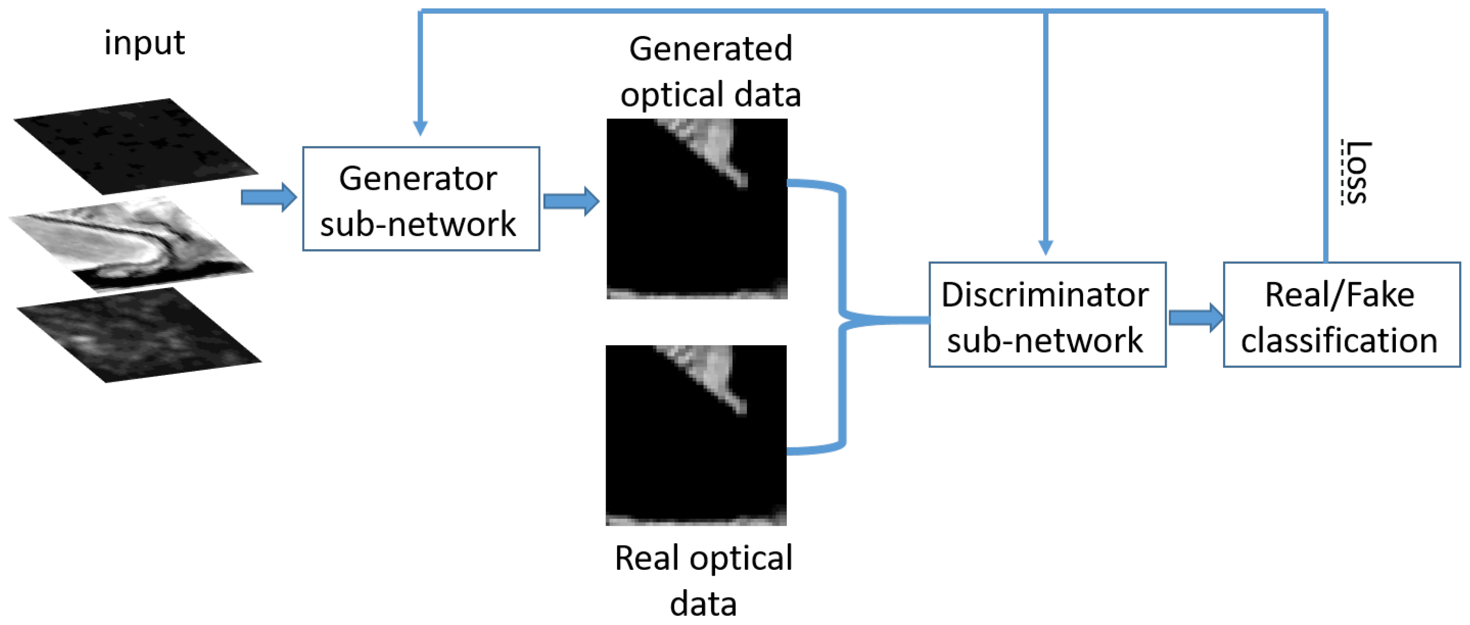
The cGAN network requires the simultaneous training of generative and discriminative networks. As stated in the preceding section, the generator produces a fake image from the input data, and the discriminator tries to classify the input-fake pair and input-real pair. The discriminator is first trained to improve the classification accuracy. A trained discriminator is then used to train the generative network. The process alternates until the end. The flowchart of the proposed cGAN is presented in Figure 3. The CNN model (described in Section 2.2) is regarded as the generative sub-network and incorporated in an adversarial framework, regularized by a discriminative sub-network.
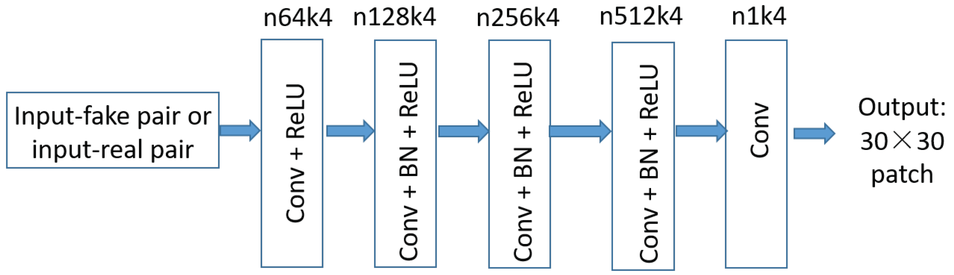
The discriminative sub-network described in Figure 4 is borrowed from [6] with to capture high-frequencies and reduced parameters. The discriminative sub-network consists of five layers and the components of each layer are illustrated in Figure 4. What we need to clarify is that the striding size of the first three layers are set as and for the last two layers. For the input image with , the spatial size of each output ranges for all layers and the output of the network is a image between the range [0, 1]. At last, this output image is adopted to classify the input pair to be real or fake.
2.4. Implementation Issues
Previous works on GAN have demonstrated the importance of using Gaussian noise as input in the generative network. In this work on cGAN, the input is x and the noise is absorbed into the dropout part, which can also produce reasonable results [6]. In our experiments, the dropout rate is set as . Mini-batch stochastic gradient decent with Adam solver is adopted to train the particular model. The model is trained on 200 epochs with batch size 1 and learning rate . As suggested in literature [20], in the loss objective (3) is set to 100 to encourage both reconstruction accuracy and object sharpness, simultaneously.
3. Dataset Description and Experimental Setting
3.1. Dataset
Sentinel-1 and -2 data (download website: https://scihub.copernicus.eu/dhus/) were adopted in our experiments to confirm the possibility of optical simulation from SAR data. The data were pre-processed and co-registered by Sentinel Application Platform (SNAP) software provided by European Space Agency (ESA) [21]. We processed the SAR image with the flowchart of calibration-despeckling-Range Doppler Terrain, and two bands of VV (for vertical transmit and vertical receive)/VH (for vertical transmit and horizontal receive) intensities with a pixel spacing of 10 m. For Sentinel-2 data, we chose four bands (R-G-B-NIR) with a ground sampling distance of 10 m for the experiments. The SAR and optical images were co-registered by reprojection; SAR and Optical data pairs from three areas (Iraq, Jianghan, and Xiangyang) were used in the experiments. The acquisition time for each image is presented in Table 1. The absolute difference in acquisition time between S1 and O1 (or, S2 and O2) is ensured to be less then five days. Images from Iraq, Jianghan and Xiangyang are of size , and , respectively. An earthquake happened in the Iraq area between time T1 and T2, which caused many changes in the terrain. Jianghan and Xiangyang images are from two similar areas of China and were sensed at the nearby time. The O2 images of these areas are presented in Figure 5.
3.2. Training and Test Setup
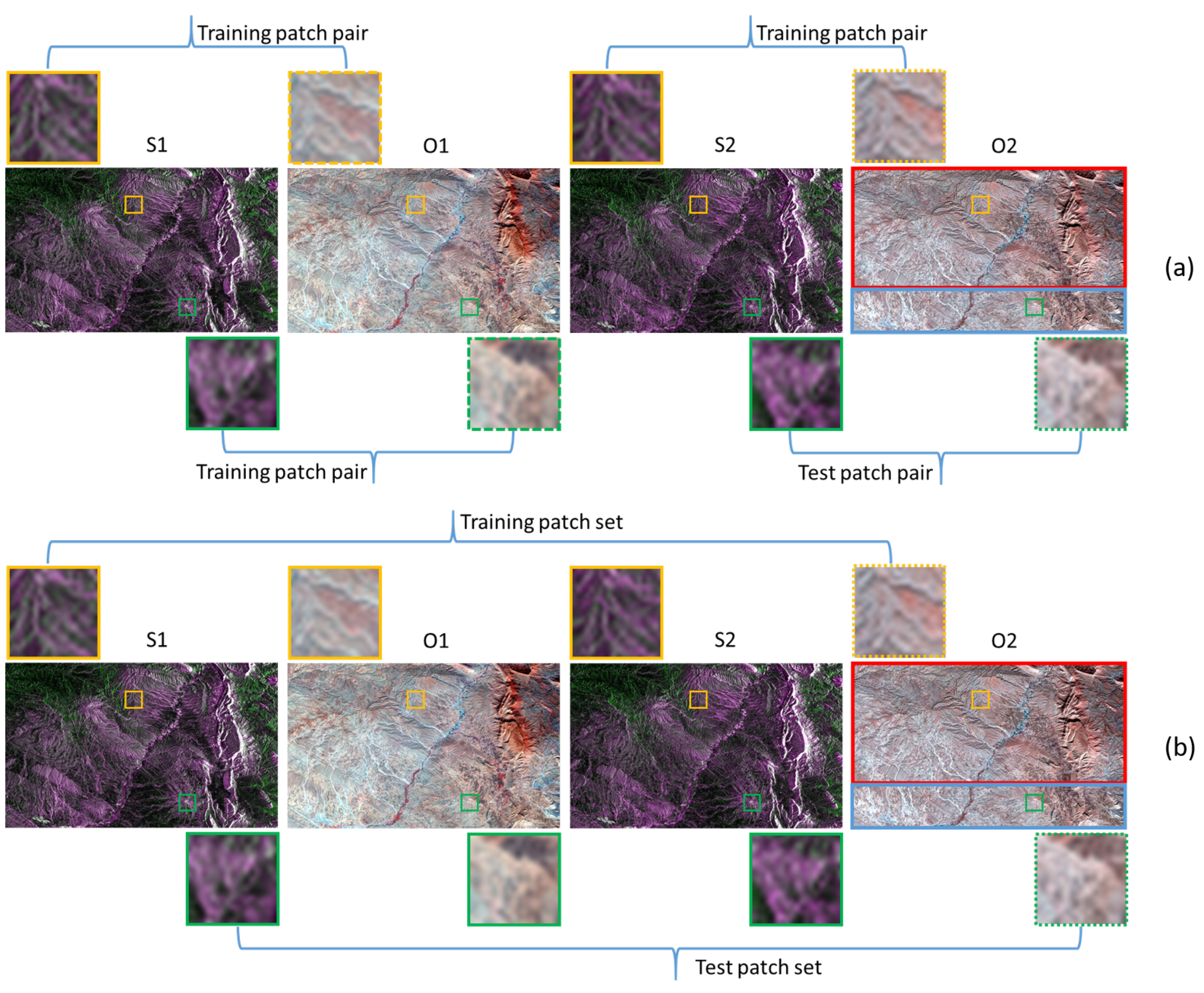
The images were segmented into non-overlapping patch pairs of spatial size . The training data were then selected from the area inside the red rectangle, and the test data from the blue ones. Figure 6 illustrates the training and test patch pairs generation with the Iraq dataset. The purpose of Task A and Task B is to simulate the blue rectangle area of O2 image. For Task A, the image patch pair consists of two patches cropped from the same location of S1-O1 or S2-O2 images. Since Task A only needs SAR image to generate the optical image, the patch pairs from the blue rectangle are adopted as test samples, and the rest are regarded as training samples, as presented in Figure 6a. For Task B, each patch set consists of four patches cropped from the same area of S1, O1, S2 and O2. Task B needs S1, O1 and S2 as input, and O2 as output. Examples of training and test patch sets are presented in Figure 6b. The number of training and test patch sets of Task B are summarized in Table 2. Models specific to each test area were designed according to the respective training dataset as per the details given below.
Case (1) In this case, we evaluate the O2 image simulation performance of different tasks and methods, with the training and test patch pairs/sets fixed. The test patches were taken from Iraq image. The optical image simulation results of Tasks A and B were verified with different models, i.e., CNN (the generation model described in Figure 2) and cGAN. To make the fair comparison, the training patch pairs of Task A were from the whole Iraq image pairs of T1 and areas of T2 marked with the red rectangle, with 1221 pairs in total. For Task B, the training patch sets were only from the areas of Iraq image marked with the red rectangle. The four methods were denoted as CNN (Task A with CNN), cGAN (Task A with cGAN), MTCNN (Task B with CNN), and MTcGAN (Task B with cGAN), respectively. In addition, the pix2pix method mentioned in the reference [10] is adopted as the state-of-the-art comparison method.
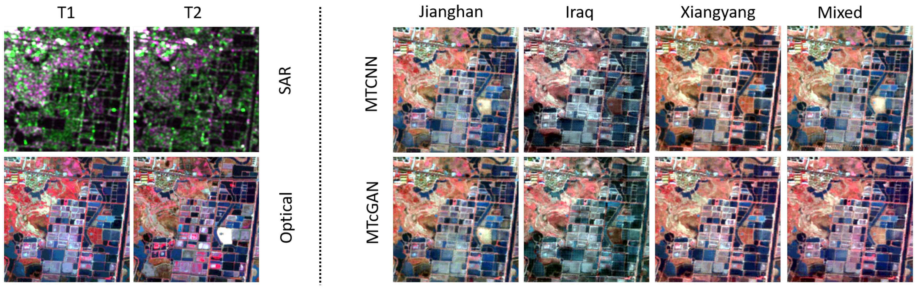
Case (2) The purpose of the second experimental study is to investigate the influence of different training sets for the final optical image simulation. The test patches were taken from Jianghan image. In this case, we performed only Task B, and train MTCNN and MTcGAN models with four different training sets. For the first three sets, the samples were selected from the training parts of the Jianghan, Iraq, and Xiangyang images, respectively. In this case, the simulated optical images of MTCNN and MTcGAN methods can be with different training sets. We also added the whole training patches together to formulate the final training set, denoted as “Mixed”.
3.3. Evaluation Index
In this paper, three evaluation indicators: the peak signal-to-noise ratio (PSNR), the structural similarity (SSIM), and the mean spectral angle (MSA) were used to assess the quality of the simulated optical image. For the multispectral image, we calculated the values of PNSR and SSIM of each band between simulated optical image and the reference image, and determined the average [22].
4. Results
The training program was completed on a single GTX1080 GPU. The PSNR, SSIM and MSA values of different simulation results for Case 1 are evaluated and listed in Table 3. The values of the three indices for input O1 data are regarded as the baseline for the other sets. The best of the values for each quality index in the table are shown in bold. From visual and quantitative evaluation results, the cGAN method can achieve better results than the method of [10], demonstrating the advantage of ResNets in our model. Table 3 also shows that CNN and cGAN achieve lower values for all three quality indices compared to the baseline. This essentially concludes that Task A, which describes the optical image simulation from single SAR imagery, fails to predict the image. On the other hand, Task B related methods, i.e., MTCNN and MTcGAN, are found to achieve higher values for each index type compared to the baseline. The results indicate that, compared to the input images, MTCNN and MTcGAN can successfully simulate the optical images. Furthermore, higher index value of MTcGAN than that of MTCNN suggests the advantage of an adversarial network in our simulation task. The training time of different methods are also presented in Table 3. Task A related methods have light networks, but more training samples compared to Task B. The differences of the training time between these methods are finite.
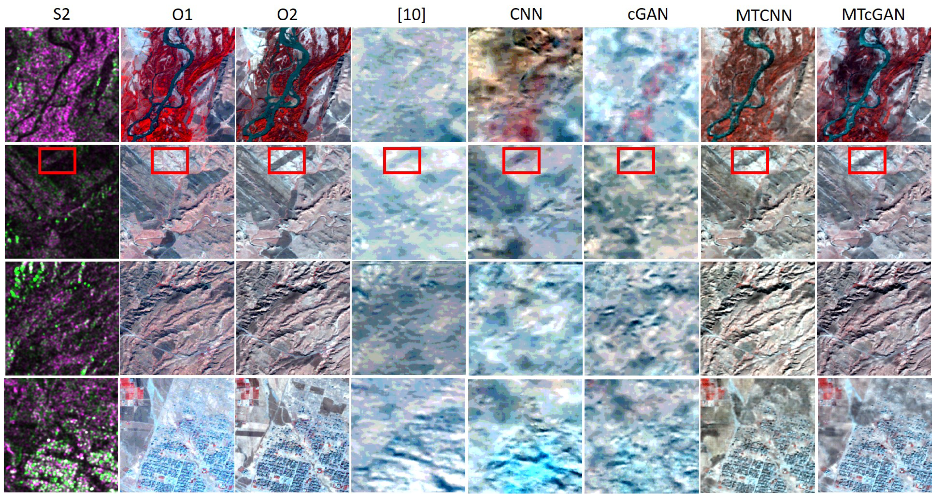
Figure 7 shows several patches of input S2 and O1, and output reference O2, compared with our optical image simulation results. In Figure 7, MTCNN and MTcGAN demonstrate much better results than that of CNN and cGAN from a visual perspective. In fact, SAR image and optical image being totally different from each other, it is extremely difficult to learn a mapping between the two. The optical simulation results of Task A and method [10] presented in Figure 7 are hence blurred, and we can not distinguish objects from these simulated images. However, with multi-temporal fusion based optical simulation of Task B, one can learn the changed information between S1 and S2, and then accordingly reconstruct the change on the basis of O1 image. As illustrated in the red rectangle of Figure 7, one can see that a change has happened between O1 and O2. Our goal is to pass this change from the SAR image to the optical image, and then reconstruct the same in the simulated O2 image. Following this strategy, the complexity of Task B can be significantly reduced, and the optical image can thus be successfully simulated.
We also investigated the influence of different training samples on the final optical image simulation results of MTCNN and MTcGAN methods in Case 2. Table 4 presents the values for the three quality indices, and Figure 8 illustrates the simulated optical images of different methods from different training sets. It can be easily seen that the two methods with Jianghan image as training samples results in the best values and visual quality. On the other hand, MTCNN and MTcGAN methods with an Iraq image as training samples have the lowest PSNR, SSIM and MSA values. Interestingly, the simulation results with Iraq training samples are of high visual quality, but with a significant change in spectral information compared to the reference optical image. This model has thus simulated a new style of optical image, guided by the Iraq training set. The main reason behind the observed result is that the test samples are composed of flat areas, even though the Iraq training samples are filled with mountains. Xiangyang training samples are more similar to the test Jianghan image patches. As a result, the models with Xiangyang training samples can produce much better results than that with the Iraq samples. Thus, selection of training samples can largely influence the final simulation results; more similarity between test data of the training samples results in better optical image simulation. Accumulation of training sets is one way to improve the reliability of simulation results. However, the simulation results obtained with the whole training data together are worse than the one with only Jianghan data.
The experimental part is thus concluded with the verification of two hypotheses. First, a multi-temporal fusion based optical simulation in Task B is valid and effective. Second, a GAN based method can produce better results than that of CNN. However, the corresponding simulation results are not so perfect. As illustrated in the red rectangle of Figure 7, MTcGAN, standing for the best method, can only simulate a blurred object of the change information compared to the reference one. Additionally, the model is sensitive to the training samples. If the training samples are improper, it may lead to the production of some fake results with the trained model. From another aspect, if we simply add the whole samples for training, we can obtain the satisfied results. However, it leaves much room for the performance improvement by mitigating the negative effects from improper samples.
5. Conclusions
We have investigated the possibility of optical image simulation from single SAR imagery and multi-temporal SAR-optical images, in this paper. Two deep learning based methods have been designed for the said tasks, i.e., CNN with ResNets and cGAN. We tested our models on Sentinel-1 and -2 datasets and compared them with the state-of-the-art method and drew the following conclusions. First, multi-temporal data fusion based optical image simulation can successfully generate the optical images. The simulated optical images show more similarity to the reference optical images, both in visual and quantitative evaluation, compared to those obtained by the state-of-the-art method and the input optical images. Second, an adversarial network is proved useful and effective in our task.
Despite the satisfactory performance of multi-temporal fusion model with the cGAN method, there is still much room for improvement. The simulated optical images, especially in the changing part of S1 and S2 images, are blurred and need improvement. Selection of the training samples is also a big concern for our model since, without proper samples, the models may create fake optical images. Finally, in our model, we have chosen only two time periods of information, i.e., T1 and T2, and it may be possible to choose a few more to obtain better simulation results.
Author Contributions
W.H. was responsible for the method design, experiments and analysis, and drafting of the manuscript. N.Y. designed the model and made valuable suggestions to improve the quality of the paper.
Funding
This work was supported by the Japan Society for the Promotion of Science (KAKENHI 18K18067).
Acknowledgments
The authors would like to thank the handling editors and anonymous reviewers for their helpful comments.
Conflicts of Interest
The authors declare no conflict of interest.
Abbreviations
The following abbreviations are used in this manuscript:
| CNN | convolutional neural network |
| cGAN | conditional generative adversarial network |
| ResNets | residual networks |
| MTCNN | multi-temporal CNN |
| MTcGAN | multi-temporal cGAN |
References
- Drusch, M.; Del Bello, U.; Carlier, S.; Colin, O.; Fernandez, V.; Gascon, F.; Hoersch, B.; Isola, C.; Laberinti, P.; Martimort, P.; et al. Sentinel-2: ESA’s Optical High-Resolution Mission for GMES Operational Services. Remote Sens. Environ. 2012, 120, 25–36. [Google Scholar] [CrossRef]
- Hagolle, O.; Huc, M.; Pascual, D.V.; Dedieu, G. A multi-temporal method for cloud detection, applied to FORMOSAT-2, VENuS, LANDSAT and SENTINEL-2 images. Remote Sens. Environ. 2010, 114, 1747–1755. [Google Scholar] [CrossRef] [Green Version]
- Cheng, Q.; Shen, H.; Zhang, L.; Yuan, Q.; Zeng, C. Cloud removal for remotely sensed images by similar pixel replacement guided with a spatio-temporal MRF model. ISPRS J. Photogramm. Remote Sens. 2014, 92, 54–68. [Google Scholar] [CrossRef]
- Torres, R.; Snoeij, P.; Geudtner, D.; Bibby, D.; Davidson, M.; Attema, E.; Potin, P.; Rommen, B.; Floury, N.; Brown, M.; et al. GMES Sentinel-1 mission. Remote Sens. Environ. 2012, 120, 9–24. [Google Scholar] [CrossRef]
- Verdoliva, L.; Gaetano, R.; Ruello, G.; Poggi, G. Optical-Driven Nonlocal SAR Despeckling. IEEE Geosci. Remote Sens. Lett. 2015, 12, 314–318. [Google Scholar] [CrossRef]
- Isola, P.; Zhu, J.Y.; Zhou, T.; Efros, A.A. Image-To-Image Translation With Conditional Adversarial Networks. In Proceedings of the IEEE Conference on Computer Vision and Pattern Recognition (CVPR), Honolulu, HI, USA, 21–26 July 2017. [Google Scholar]
- Merkle, N.; Auer, S.; Mller, R.; Reinartz, P. Exploring the Potential of Conditional Adversarial Networks for Optical and SAR Image Matching. IEEE J. Sel. Top. Appl. Earth Obs. Remote Sens. 2018, PP, 1–10. [Google Scholar] [CrossRef]
- Wang, P.; Patel, V.M. Generating high quality visible images from SAR images using CNNs. In Proceedings of the Radar Conference (RadarConf18), Oklahoma City, OK, USA, 23–27 April 2018; pp. 570–575. [Google Scholar]
- Merkle, N.; Fischer, P.; Auer, S.; Müller, R. On the possibility of conditional adversarial networks for multi-sensor image matching. In Proceedings of the 2017 IEEE International Geoscience and Remote Sensing Symposium (IGARSS), Fort Worth, TX, USA, 23–28 July 2017; pp. 2633–2636. [Google Scholar]
- Schmitt, M.; Hughes, L.H.; Zhu, X.X. The SEN1-2 Dataset for Deep Learning in SAR-Optical Data Fusion. arXiv, 2018; arXiv:1807.01569. [Google Scholar]
- Ioffe, S.; Szegedy, C. Batch Normalization: Accelerating Deep Network Training by Reducing Internal Covariate Shift. In Proceedings of the 32nd International Conference on Machine Learning, PMLR, Lille, France, 6–11 July 2015; Volume 37, pp. 448–456. [Google Scholar]
- He, K.; Zhang, X.; Ren, S.; Sun, J. Deep Residual Learning for Image Recognition. In Proceedings of the IEEE Conference on Computer Vision and Pattern Recognition (CVPR), Las Vegas, NV, USA, 26 June–1 July 2016; pp. 770–778. [Google Scholar]
- Krizhevsky, A.; Sutskever, I.; Hinton, G.E. ImageNet Classification with Deep Convolutional Neural Networks. In Advances in Neural Information Processing Systems 25; ACM: New York, NY, USA, 2012; pp. 1097–1105. [Google Scholar]
- Zhang, K.; Zuo, W.; Chen, Y.; Meng, D.; Zhang, L. Beyond a Gaussian Denoiser: Residual Learning of Deep CNN for Image Denoising. IEEE Trans. Image Process. 2017, 26, 3142–3155. [Google Scholar] [CrossRef] [PubMed] [Green Version]
- Yan, L.; Zhu, R.; Liu, Y.; Mo, N. TrAdaBoost Based on Improved Particle Swarm Optimization for Cross-Domain Scene Classification With Limited Samples. IEEE J. Sel. Top. Appl. Earth Obs. Remote Sens. 2018, 99, 1–17. [Google Scholar] [CrossRef]
- Li, Y.; Zhang, Y.; Huang, X.; Ma, J. Learning Source-Invariant Deep Hashing Convolutional Neural Networks for Cross-Source Remote Sensing Image Retrieval. IEEE Trans. Geosci. Remote Sens. 2018, 99, 1–16. [Google Scholar] [CrossRef]
- Radford, A.; Metz, L.; Chintala, S. Unsupervised representation learning with deep convolutional generative adversarial networks. arXiv, 2015; arXiv:1511.06434. [Google Scholar]
- Johnson, J.; Alahi, A.; Fei-Fei, L. Perceptual Losses for Real-Time Style Transfer and Super-Resolution. In Computer Vision ECCV; Springer: Cham, Switzerland, 2016; pp. 694–711. [Google Scholar]
- Goodfellow, I.; Pouget-Abadie, J.; Mirza, M.; Xu, B.; Warde-Farley, D.; Ozair, S.; Courville, A.; Bengio, Y. Generative adversarial nets. In Advances in Neural Information Processing Systems; ACM: New York, NY, USA, 2014; pp. 2672–2680. [Google Scholar]
- Ghamisi, P.; Yokoya, N. IMG2DSM: Height Simulation from Single Imagery Using Conditional Generative Adversarial Nets. IEEE Trans. Geosci. Remote Sens. Lett. 2018, PP, 1–5. [Google Scholar] [CrossRef]
- Zuhlke, M.; Fomferra, N.; Brockmann, C.; Peters, M.; Veci, L.; Malik, J.; Regner, P. SNAP (Sentinel Application Platform) and the ESA Sentinel 3 Toolbox. In Proceedings of the Sentinel-3 for Science Workshop, Venice, Italy, 2–5 June 2015; Volume 734, p. 21. [Google Scholar]
- He, W.; Zhang, H.; Zhang, L.; Shen, H. Total-Variation-Regularized Low-Rank Matrix Factorization for Hyperspectral Image Restoration. IEEE Trans. Geosci. Remote Sens. 2016, 54, 178–188. [Google Scholar] [CrossRef]
Figure 1.
Illustration of two optical simulation tasks.

Figure 2.
Illustration of the CNN generation network.

Figure 3.
The flowchart of the cGAN architecture.

Figure 4.
Illustration of the discriminative sub-network.

Figure 5.
O2 images of Iraq, Jianghan and Xiangyang pairs. The training patches are selected from the red rectangle and the test patches are from the blue area.
Figure 5.
O2 images of Iraq, Jianghan and Xiangyang pairs. The training patches are selected from the red rectangle and the test patches are from the blue area.

Figure 6.
Illustration of training and test patch pairs with Iraq dataset for (a) Task A, and (b) Task B.
Figure 6.
Illustration of training and test patch pairs with Iraq dataset for (a) Task A, and (b) Task B.

Figure 7.
Simulated images of different methods in Case 1, companied with the input images (S2 and O1) and output reference image (O2).
Figure 7.
Simulated images of different methods in Case 1, companied with the input images (S2 and O1) and output reference image (O2).

Figure 8.
Simulated images of different methods in Case 2. The input images (S1, S2 and O1) and output reference image (O2) on the left side, and simulated images with different training samples on the right side.
Figure 8.
Simulated images of different methods in Case 2. The input images (S1, S2 and O1) and output reference image (O2) on the left side, and simulated images with different training samples on the right side.


Table 1.
Sensing time of optical and SAR image pairs used in the experiments.
| Y-M-D | S1 | O1 | S2 | O2 |
|---|---|---|---|---|
| Iraq | 12 November 2017 | 10 November 2017 | 6 December 2017 | 10 December 2017 |
| Jianghan | 14 November 2017 | 12 November 2017 | 20 December 2017 | 19 December 2017 |
| Xiangyang | 14 November 2017 | 12 November 2017 | 20 December 2017 | 19 December 2017 |
Table 2.
The training and test Patches provided by the images.
| Iraq | Jianghan | Xiangyang | |
|---|---|---|---|
| Train | 561 | 1188 | 754 |
| Test | 99 | 165 | None |
Table 3.
The evaluation values of PSNR, SSIM, MSA and training time of different methods in Case 1.
| Index | [10] | CNN | cGAN | MTCNN | MTcGAN | O1 |
|---|---|---|---|---|---|---|
| PSNR (dB) | 26.50 | 26.60 | 26.79 | 30.61 | 32.32 | 29.77 |
| SSIM | 0.6419 | 0.6477 | 0.6519 | 0.9028 | 0.9110 | 0.8528 |
| MSA | 0.6545 | 0.6769 | 0.6581 | 0.3796 | 0.3146 | 0.5529 |
| Training Time (s) | 4252 | 3747 | 4025 | 3506 | 3892 | None |
Table 4.
Simulation accuracy of MTCNN and MTcGAN with different training samples in Case 2.
| Method | Index | Jianghan | Iraq | Xiangyang | Mixed | O1 |
|---|---|---|---|---|---|---|
| PSNR | 35.08 | 29.44 | 34.30 | 34.38 | 34.01 | |
| MTCNN | SSIM | 0.9508 | 0.8585 | 0.9412 | 0.9479 | 0.9401 |
| MSA | 0.4684 | 0.8400 | 0.5138 | 0.4774 | 0.5319 | |
| PSNR | 35.25 | 31.09 | 34.44 | 34.83 | 34.01 | |
| MTcGAN | SSIM | 0.9509 | 0.8850 | 0.9413 | 0.9463 | 0.9401 |
| MSA | 0.4629 | 0.6137 | 0.5070 | 0.4649 | 0.5319 |
© 2018 by the authors. Licensee MDPI, Basel, Switzerland. This article is an open access article distributed under the terms and conditions of the Creative Commons Attribution (CC BY) license (http://creativecommons.org/licenses/by/4.0/).
Share and Cite
MDPI and ACS Style
He, W.; Yokoya, N. Multi-Temporal Sentinel-1 and -2 Data Fusion for Optical Image Simulation. ISPRS Int. J. Geo-Inf. 2018, 7, 389. https://doi.org/10.3390/ijgi7100389
AMA Style
He W, Yokoya N. Multi-Temporal Sentinel-1 and -2 Data Fusion for Optical Image Simulation. ISPRS International Journal of Geo-Information. 2018; 7(10):389. https://doi.org/10.3390/ijgi7100389
Chicago/Turabian StyleHe, Wei, and Naoto Yokoya. 2018. "Multi-Temporal Sentinel-1 and -2 Data Fusion for Optical Image Simulation" ISPRS International Journal of Geo-Information 7, no. 10: 389. https://doi.org/10.3390/ijgi7100389
Note that from the first issue of 2016, this journal uses article numbers instead of page numbers. See further details here.