Article

A Knowledge-Informed and Pareto-Based Artificial Bee Colony Optimization Algorithm for Multi-Objective Land-Use Allocation

1
Institute of Remote Sensing and Digital Earth, Chinese Academy of Sciences, Beijing 100864, China
2
Department of Geography, University of Wisconsin-Madison, Madison, WI 53706, USA
3
Key Laboratory of Virtual Geographic Environment, Nanjing Normal University, Nanjing 210097, China
4
Institute of Electronics, Chinese Academy of Sciences, Beijing 100864, China
*
Author to whom correspondence should be addressed.
ISPRS Int. J. Geo-Inf. 2018, 7(2), 63; https://doi.org/10.3390/ijgi7020063
Submission received: 18 December 2017 / Revised: 4 February 2018 / Accepted: 6 February 2018 / Published: 12 February 2018

Abstract

:
Land-use allocation is of great significance in urban development. This type of allocation is usually considered to be a complex multi-objective spatial optimization problem, whose optimized result is a set of Pareto-optimal solutions (Pareto front) reflecting different tradeoffs in several objectives. However, obtaining a Pareto front is a challenging task, and the Pareto front obtained by state-of-the-art algorithms is still not sufficient. To achieve better Pareto solutions, taking the grid-representative land-use allocation problem with two objectives as an example, an artificial bee colony optimization algorithm for multi-objective land-use allocation (ABC-MOLA) is proposed. In this algorithm, the traditional ABC’s search direction guiding scheme and solution maintaining process are modified. In addition, a knowledge-informed neighborhood search strategy, which utilizes the auxiliary knowledge of natural geography and spatial structures to facilitate the neighborhood spatial search around each solution, is developed to further improve the Pareto front’s quality. A series of comparison experiments (a simulated experiment with small data volume and a real-world data experiment for a large area) shows that all the Pareto fronts obtained by ABC-MOLA totally dominate the Pareto fronts by other algorithms, which demonstrates ABC-MOLA’s effectiveness in achieving Pareto fronts of high quality.

1. Introduction

Land-use allocation is a complex multi-objective optimal problem (MOOP) in which certain land-use types are allocated to proper units by considering multiple objectives [1,2,3,4,5,6,7,8]. When modeling and solving such problems, the goal is to find a set of optimal solutions that are essentially non-inferior [9] rather than a single best solution [10,11]. Therefore, multi-objective land-use allocation (MOLA) is a difficult problem to solve.
The approaches to MOLA can be divided into two categories: scalarization and Pareto [3,5]. The goal of scalarization, the oldest and most direct approach [3], is to transform a multi-objective problem into a single-objective problem using a priori knowledge and then solve the simpler single-objective problem [12]. The commonly-used transformation methods include weighted sum [13], goal programming [14] and ε-constraint [15]. In general, these types of methods are not able to evaluate the contributions of all the objectives to a solution and may fail to find important solutions if the transformation parameters are not properly designed [16]. In order to get a set of optimal solutions, multiple executions of single-objective optimization are conducted by using different sets of transformation parameters such as weights. For example, Huang et al. [17] proposed a novel approach that adaptively alters the objective weights according to the largest unexplored feasible region to produce a set of solutions. However, because multiple single-objective optimizations have to be repeatedly carried out, the whole procedure could be computationally expensive.
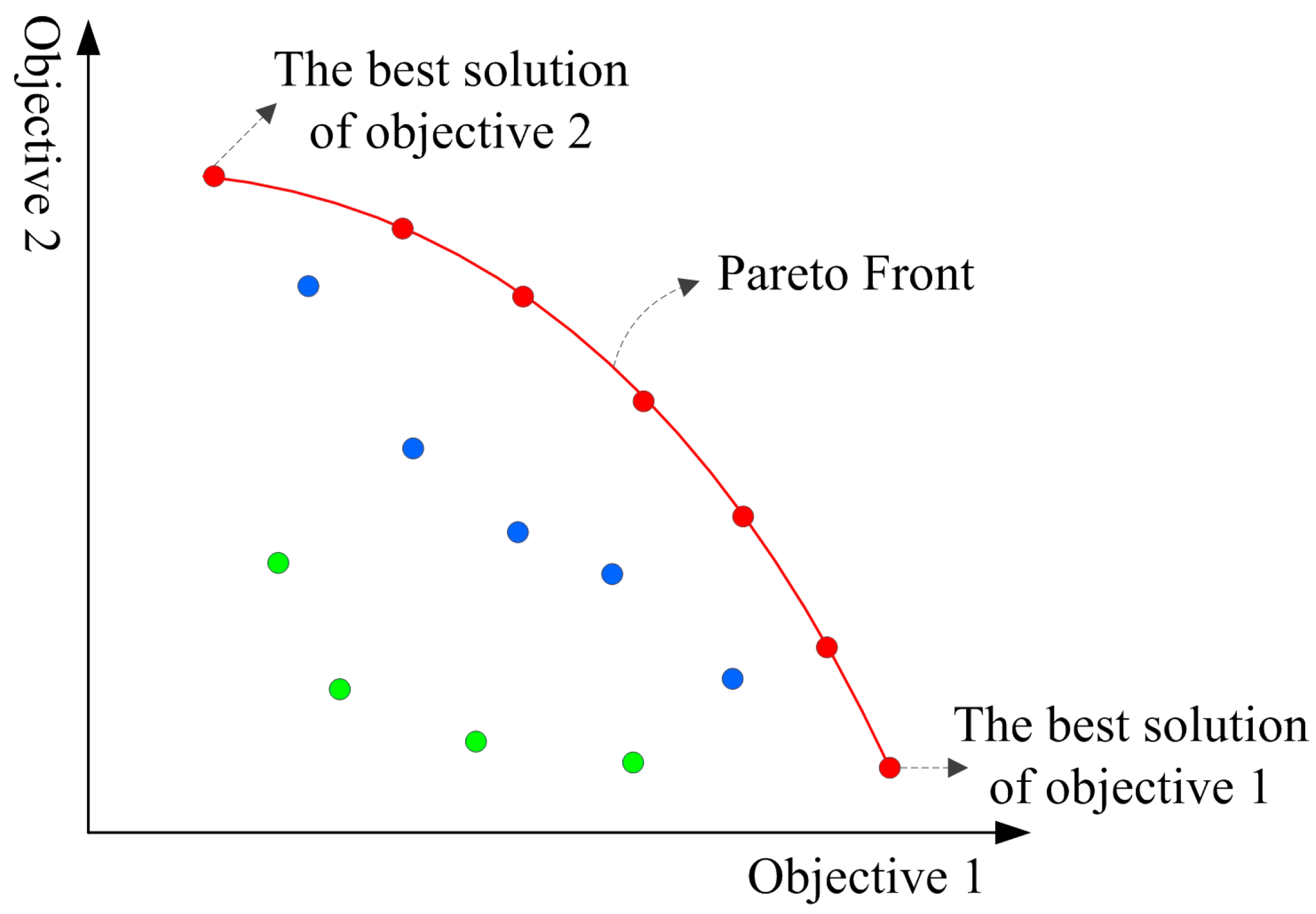
The Pareto approach originated from the concept of Pareto optimality (Pareto, 1965, originally published in 1896). A solution is Pareto optimal when no other solution is as good or better with respect to all objective functions and when it is also strictly better in at least one objective function than any other solution [18]. A Pareto-optimal solution set or Pareto front (shown in Figure 1) can be obtained by using the Pareto approach integrated with heuristic algorithms [19,20,21,22,23,24,25], which involves constructing new solutions iteratively and preserving Pareto-optimal solutions selectively. The solutions on the Pareto front reflect different tradeoffs among the multiple objectives [5]. Because the Pareto approach has the advantage that an entire Pareto front can be achieved by only one computation, it can better meet the requirements of multi-objective optimal decision-making.
Recently, studies on MOLA have applied some Pareto-based heuristic algorithms, including evolutionary algorithms [7,18,26,27], simulated annealing (SA) [3] and the artificial immune system (AIS) [28]. Duh and Brown [3] developed a knowledge-informed Pareto simulated annealing approach (PSA) to solve the MOLA problem. Based on an initial solution set that includes the best solution of each single objective function and some random feasible solutions, PSA can obtain a Pareto front by iteratively executing the following steps: (1) new solution construction, (2) dominance assessments, (3) Pareto solution set updating, (4) objective-weight calculations and (5) new solution acceptance judgments. Meanwhile, PSA defined two knowledge-informed rules—the compactness rule and the suitability rule—to monitor the construction of new solutions. However, these rules were used only on the solutions with the largest weight values in any objective direction, which resulted in limited improvement of the qualities of all new solutions.
Huang et al. [28] proposed an improved artificial immune system method for multi-objective land-use allocation (AIS-MOLA). Initially, based on each random solution, the mutation strategy of random exchange and the selection strategy of compromise programming [29] were used to generate and preserve new solutions. After cloning some non-dominated solutions, new solutions were constructed using the crossover strategy. By such iterative calculations, the Pareto front can be obtained. Experiments revealed that AIS-MOLA achieved better results in both simulated and practical land-use allocation than PSA [3]. However, because only completely random strategies were used in the phase of new solution construction and no auxiliary knowledge was imported to aid in navigating the spatial search to areas where global optima were located, we believe that there is still considerable room for improvement in the quality of the Pareto front for multi-objective land-use allocation.
Generally speaking, there is still room for improvement in the quality of the Pareto front obtained for multi-objective land-use allocation. The main reasons for this can be understood from the following two perspectives. First, the adopted heuristic algorithms have specific limitations in terms of optimization. The genetic algorithm (GA) generates new solutions (offspring) using crossover and mutation manipulations based on the parents’ solutions with good functional fitness, which can reduce the genetic diversity of the population to a certain extent. Thus, GA is usually deficient because of premature convergence, a phenomenon in which the algorithm falls into local optimal solutions and cannot escape them [30]. The local search algorithm, for example, SA, generates new solutions by searching the adjacent space of a single solution; thus, the quality of these solutions is strongly dependent on the initial solutions and their neighborhood structures. Consequently, SA can also easily fall into locally optimal solutions. Moreover, the AI algorithm in [28] also used the strategy of constructing new solutions from good solutions by crossover manipulation, thus introducing a defect similar to that of GA. Second, the currently-used strategies for generating new solutions lack effective inspiration by auxiliary knowledge. Effective utilization of auxiliary knowledge of natural geography or spatial structure can significantly improve the effectiveness and efficiency of spatial optimization because such knowledge is useful in reducing the scale of the search space and preventing unproductive searches [3]. However, from the works mentioned above, it is clear that most of the solution’s neighborhood searches in a population adopted completely random strategies to construct new solutions, and auxiliary knowledge was rarely used.
Considering the above two problems, some improvements can be made from the following two aspects. To solve the first problem, we can introduce the artificial bee colony (ABC) algorithm, which is an efficient optimization algorithm that, in most cases, performs better than algorithms such as GA, AIS and particle swarm optimization (PSO) [31,32]. Moreover, it has been successfully used to tackle the problem of single-objective land-use allocation (SOLA) to obtain one optimal solution [33]. For the second problem, introducing a multi-objective spatial search strategy informed by auxiliary knowledge could guide the generation of all new solutions. For example, if a type i land-use needs to be allocated in a multi-objective maximization problem, auxiliary knowledge such as the neighborhood information could be used to select spatial units with increased functional values after compromising multiple objectives when the units are assigned type i . These selected units could be treated as a new size-reduced feasible solution space, which would be helpful for efficiently constructing new solutions and improving their qualities.
Therefore, to combine these two improvements and obtain better Pareto solutions of land-use allocation, this paper utilizes the ABC to solve this multi-objective spatial optimization problem and auxiliary spatial knowledge to improve ABC’s spatial search ability.
The remainder of this paper is arranged as follows. Section 2 theoretically and briefly introduces the Pareto optimization concept, the land-use allocation model and the ABC algorithm. Section 3 expounds on the proposed method, ABC-MOLA, in detail. Section 4 describes both simulated and practical experiments conducted to validate the optimization ability of ABC-MOLA. Finally, a substantial discussion and the conclusion are presented in Section 5 and Section 6, respectively.

2. Theory

2.1. Pareto Optimization

A maximum unconstrained multi-objective optimization problem can be defined as follows.
max F ( x ) = [ f 1 ( x ) , f 2 ( x ) , f M ( x ) ] T M
S.t.
x = [ x 1 , x 2 , x D ] T S
where x and f ( x ) are a solution and its objective function, respectively; M and D are the numbers of objective functions and decision variables, respectively; and S is a D-dimensional feasible-solution decision space. Formula (1) represents a set of objective functions that map the decision space to an objective space.
Based on this definition of the optimization problem, some definitions concerning Pareto optimization are given below and depicted in Figure 1, in which dots of the same color have the same dominance. The red dots are the Pareto solutions on the Pareto front that dominate the blue and green dots, while the blue dots dominate the green dots.
Definition 1.
(Pareto dominance). For any two solution vectors u , v Ω , u dominates v if and only if i = 1 , 2 , m , u i v i j = 1 , 2 , m , u j > v j , which can be denoted by u v .
Definition 2.
(Pareto-optimal solution). A solution x * Ω is called a Pareto-optimal or non-dominated solution if and only if ¬ x Ω : x x * .
Definition 3.
(Pareto-optimal solution set, or Pareto front). The set of all Pareto-optimal solutions P S = { x * | ¬ x Ω   :   x x * } is called the Pareto-optimal solution set. The region formed by all the objective-function values of Pareto-optimal solutions P F = { F ( x * ) | x * P S } is called the Pareto front.

2.2. Land-Use Allocation Model

Land-use allocation usually includes K land-use types in a two-dimensional study area of R rows and C columns. Each cell ( i , j ) of these data will be assigned a land-use type. This paper considers two commonly-used objectives: spatial suitability and compactness; thus, the multi-objective optimization problem can be modeled as follows.
Objective   1 :   Maximize   S u i t a b i l i t y = S u i t t o t a l S u i t min S u i t max S u i t min
Objective   2 :   Maximize   C o m p a c t n e s s = C o m t o t a l C o m min C o m max C o m min  
S.t.
S u i t t o t a l = i = 1 R j = 1 C k = 1 K S u i t i j k x i j k
S u i t max = i = 1 R j = 1 C max { S u i t i j k } , k = 1 , K
S u i t min = i = 1 R j = 1 C min { S u i t i j k } , k = 1 , K
C o m t o t a l = i = 1 R j = 1 C k = 1 K C o m i j k x i j k
C o m i j k = 4 x i 1 , j , k x i + 1 , j , k x i , j 1 , k x i , j + 1 , k , k = 1 , , K , i = 1 , , R , j = 1 , , C .
C o m max = k = 1 K 2 π A r e a k π
C o m min = k = 1 K 4 × A r e a k
i = 1 R j = 1 C x i j k = A r e a k , k = 1 , , K .
k = 1 K x i j k = 1 , i = 1 , , R , j = 1 , , C , x i j k { 0 , 1 } .
In this model, the objective values of the two functions should be normalized to the range [ 0 , 1 ] using a linear method. Formula (3) aims to maximize the linearly-normalized value of spatial suitability, S u i t t o t a l (Formula (5)), which is the sum of all cells’ suitability values after being allocated certain types. S u i t i j k is the suitability of cell ( i , j ) being assigned to land-use type k , and x i j k is a binary variable. When x i j k = 1 , a land-use of type k is allocated to cell ( i , j ) ; otherwise, x i j k = 0 . S u i t max and S u i t min are the maximum and minimum suitability values of the whole region, respectively, as shown in Formulas (6) and (7).
Meanwhile, Formula (4) is the objective function for maximizing spatial compactness, and it equals the linearly-normalized value of the compactness of the spatial pattern of the entire region after land-use allocation. For a constant area, a shorter perimeter implies greater compactness; therefore, the sum of the polygons’ perimeters in the research region, C o m t o t a l (Formula (8)), can be used to represent land-use compactness. C o m i j k (Formula (9)) is the perimeter of the polygon in which cell ( i , j ) is assigned to type k . The ideal land-use compactness (i.e., the maximum value of C o m max ) can be defined as shown in Formula (10) because, when a polygon is more like a circle, its perimeter is smaller; thus, its compactness is greater. In contrast, when each cell’s type is different from those of its four neighboring cells, the region has the lowest possible compactness, C o m min , as shown in Formula (11). In addition, Formulas (12) and (13) are regular restrictions in the land-use allocation problem: (12) restricts the areas of each land-use type, and (13) requires that each cell be assigned only one type.

2.3. Artificial Bee Colony Algorithm

The ABC algorithm is a kind of swarm intelligent optimization method that was proposed by Karaboga [34]. Usually, it involves four objects: food sources, employed bees, onlooker bees and scout bees [34]. A food source corresponds to a feasible solution, and the three types of bees are used to search for new solutions around food sources.
ABC was originally designed to solve a single-objective optimization problem (SOOP). However, as ABC has developed, several multi-objective variants such as vector evaluated ABC [35] and Pareto-based ABC [36,37,38,39] have been proposed. Vector evaluated ABC [35] lets different bee swarms optimize each objective concurrently and selects the solutions with the highest fitness in each swarm as forage bees to generate new solutions. In contrast, similar to ABC for single-objective problems, Pareto-based ABC uses only one bee swarm to optimize a MOOP. However, there are three important differences between these SOOPs and MOOPs.
First, the factor that guides onlooker bees’ search directions in solution space is different. In a SOOP, it is the qualities of the solutions as represented by objective values that influence the onlooker bees’ search behaviors. A high-quality solution (better objective value) will attract more onlooker bees to forage around it. However, in a MOOP, the solutions’ objective values can no longer be directly used to guide bees’ spatial searches because it is difficult to determine that a non-dominated solution is preferable to other non-dominated solutions for the bees simply by their objective values. To avoid this limitation, Li et al. [36] chose a random non-dominated solution among several randomly-selected solutions as the food source for onlooker bees. Wang et al. [37] used tournament selection to choose the solutions with the best dominance rank and the largest crowding distance to attract onlooker bees. Akbari et al. [39] used the roulette wheel strategy to assign each onlooker to a solution according to the probabilities determined by the number of dominated solutions for each food source.
Second, the food source’s solution updating strategy is different. In a SOOP, after each bee’s neighborhood search, each food source should be updated by the solution with higher quality, and a greedy search strategy can be used. However, in a MOOP, if both the newly-generated and the original solutions are non-dominated, it is difficult to determine which one is more advantageous to retain. To solve this problem, Li et al. [36] used a random strategy to select one solution as the updated solution. Akbari et al. [39] chose to abandon the new solution when it could not dominate the original solution. Other researchers have preferred to save all the newly-generated solutions and allow them to participate in the global updating of the Pareto archive rather than locally updating each food source [37,38].
The third difference is in the ABC’s global solution updating after each iteration. ABCs for SOOPs retain only the solution with the best objective value, while ABCs for MOOPs usually update an external archive by making Pareto dominance judgments [36,37,38,39].

3. Methodology

Aiming at the three differences between Pareto-ABC and traditional ABC, this paper adopts three strategies to make the Pareto-ABC suitable for MOLA: (1) a crowding distance is used as an indicator to direct the bees’ searches to the sparse region of the Pareto front to increase the diversity of the results [40]; the non-dominated solutions in a sparse region have higher probabilities of being selected as food sources by onlooker bees; (2) all newly-generated solutions in each iteration are added to the food-source set, which will be updated to realize the food source’s updating by the same operations as are used in the Pareto-archive maintenance process; (3) an external solution archive is used to save the Pareto optimal solutions, which will be globally updated by the Pareto-archive maintenance process described in Section 3.3.
Moreover, a neighborhood search strategy for Pareto optimization considering auxiliary knowledge will be proposed and explicitly described in Section 3.2; this is an important improvement of this paper for the optimization effectiveness of MOLA.

3.1. Algorithmic Procedure

In this paper, a two-dimensional matrix with R rows and C columns can be used to represent a solution [33]. 
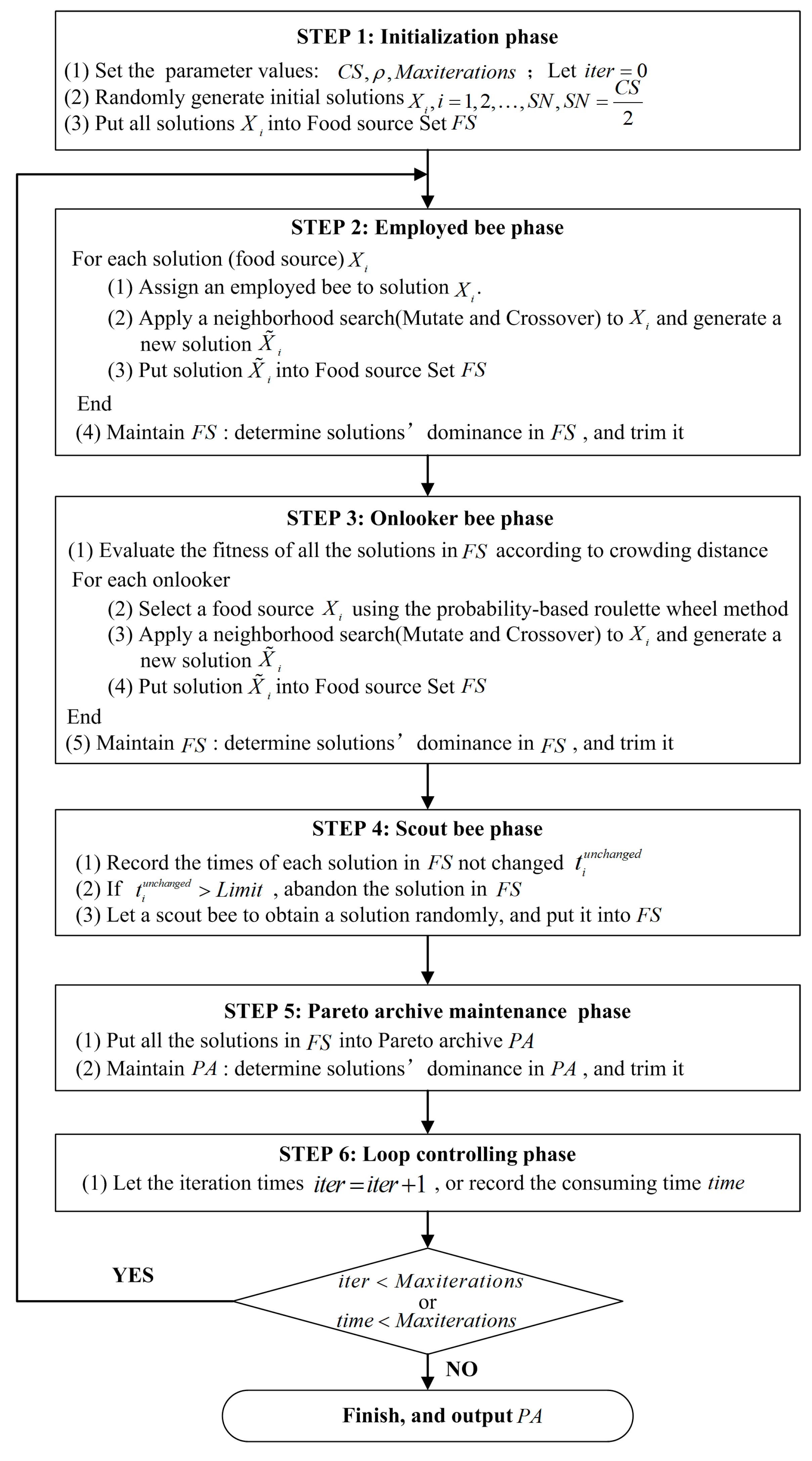
Figure 2 shows the main procedure for the ABC-MOLA algorithm.
First, all the parameter values are set and initial solutions are generated by randomly allocating a land-use type to each cell according to the planned area of each type. Then, in the employed and onlooker bee phases, new solutions are constructed using the mutation and crossover operations. In addition, the algorithm records the number of times that each solution is not updated. When this value exceeds a predefined threshold, the scout bees are activated to randomly generate a solution to replace the original. Next, all the solutions in the food-source set are added to the Pareto-solution set, and Pareto archive maintenance is conducted. Finally, when these iterative steps satisfy the convergence condition (or when the iteration time or computing time exceeds a predefined threshold), the algorithm stops.

3.2. Neighborhood Search Strategy

Bees’ neighborhood search strategies determine the optimization efficiency of the entire algorithm. Therefore, such strategies are the key parts of this study. In the ABC-MOLA algorithm, a modified mutation operator and a crossover operator are introduced to improve its spatial search capabilities.

3.2.1. Mutation Strategy

A mutation strategy, which is an iterative process, is applied to a proportion of the raster cells in the study area. During each iteration, this process allows the land-use types of a solution’s different raster cells to be exchanged to obtain a new solution with a knowledge-informed neighborhood search strategy. Then, the newly-generated solution must be compared with the original solution using the technique of compromising programming to perform the solution selection process.

Knowledge-Informed Neighborhood Search Strategy

This paper proposes two knowledge-informed rules, the compactness rule and the suitability rule, which correspond to the land-use allocation’s two objective functions. These rules govern the generation of new solutions in each bee’s neighborhood search process, so that the newly-generated solution’s quality can be improved after reallocating a land-use type to a proper raster cell. The compactness rule attempts to promote the solution with the most compact pattern in each mutation step by preferentially assigning to a randomly-selected cell the same type as the cell with the highest quantity among its four neighboring cells. When the number of neighboring cells with the same land-use type as the central cell is increased by one, the compactness increment can be quantified as 2 C o m max C o m min . In addition, the suitability rule encourages the promotion of a solution’s suitability by making the method more inclined to allocate type k , which has the highest suitability, to a randomly selected cell ( i , j ) . If the original type of cell ( i , j ) was k ' , the suitability increment is S u i t i j k S u i t i j k ' S u i t max S u i t min .
Moreover, because the objective increments of compactness and suitability can be easily quantified and the increment of the model’s utility value, such as weighted sum of the two functions, can be efficiently calculated, when generating a new solution by pseudo-random exchange in the mutation step, this increment value is a useful piece of heuristic information. The larger the increment value, the greater the probability for assigning the type to raster cell ( i , j ) . The knowledge-informed neighborhood search (KINS) strategy can greatly increase the efficiency and effectiveness of approximating the Pareto front.

Solution Selection Based on Compromising Programming

The newly-generated solution x j needs to be compared with the original solution xi to complete the solution-selection step. If x j is better than x i , x i will be replaced by x j , which can be notated as x i x j ; otherwise, x j is abandoned, and x i is retained. Subsequently, the next mutation will be carried out based on the better solution.
Usually, the traditional technique of Pareto-dominance judgment can be used to evaluate the two solutions’ qualities. However, if they are both non-dominated solutions, the traditional technique is no longer useful, and no helpful preference for solution selection will be given to obtain the Pareto front. Therefore, to overcome the problem, compromising programming can be introduced to evaluate two solutions during the mutation procedure.
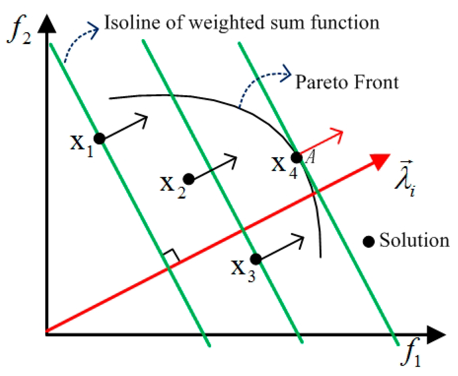
Weighted sum, a type of compromising programming, is the most direct method to tackle a multi-objective optimization problem [13]. It converts an m-dimensional multi-objective problem into a single-objective problem by weighting each objective function by a nonnegative vector λ = ( λ 1 , λ 2 , λ m ) . In a maximum multi-objective optimization problem, each bee searches around a food source to find a new solution with a larger value for a single objective function as shown in Formula (14).
max ( P ( x j ) ) = max ( i = 0 m λ i f i ( x j ) ) ,   subject   to   λ i 0 , i = 1 m λ i = 1 , i = 1 , 2 , , m
This technique is effective in guiding the spatial search in the direction of this weight vector, thus improving the mutation’s optimization efficiency. Taking m = 2 as an example, the technique can be illustrated as follows.
For any two-dimensional weight vector λ i = ( λ i 1 , λ i 2 ) , the isolines of the weighted-sum function are a series of straight lines aligned perpendicularly to λ i , as shown in Figure 3. According to (14), solution x 2 is better than x 1 and worse than x 3 ; thus, the solution retained during the mutation manipulation will move progressively further away from the origin in the direction of λ i , until the isoline of the solution’s weighted-sum function is tangent to the Pareto front (Point A in Figure 3, which is an optimal solution of problem P ( x j ) ). In the problem illustrated in Figure 3, three mutation manipulations will be executed and the solution-selection process can be recorded as x 1 x 2 x 3 x 4 .
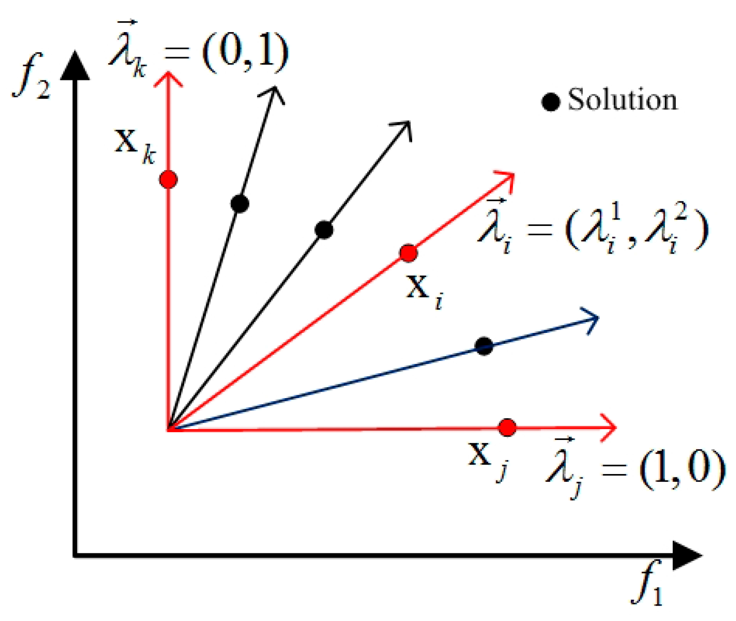
In this study, the weight vector of each solution is closely related to the spatial distribution of all solutions in the objective space, as shown in Figure 4. The weight λ i j of solution x i in the direction of objective function j is defined by Formulas (15) and (16). Note that defining the weight vector by such a method ensures that different solutions have different optimization directions (selection preferences) during the mutation operation and further ensures the diversity of the solutions in the Pareto front.
λ i j = f j ( x i ) f j min f j max f j min
S . t . { f j max = max { f j ( x i ) } f j min = min { f j ( x i ) } , i = 1 , 2 , , S N

3.2.2. Crossover Strategy

The crossover strategy is used after the mutation operation. It allows two solutions to exchange parts of their raster cells to form new solutions, which is helpful for increasing the diversity of this algorithm.
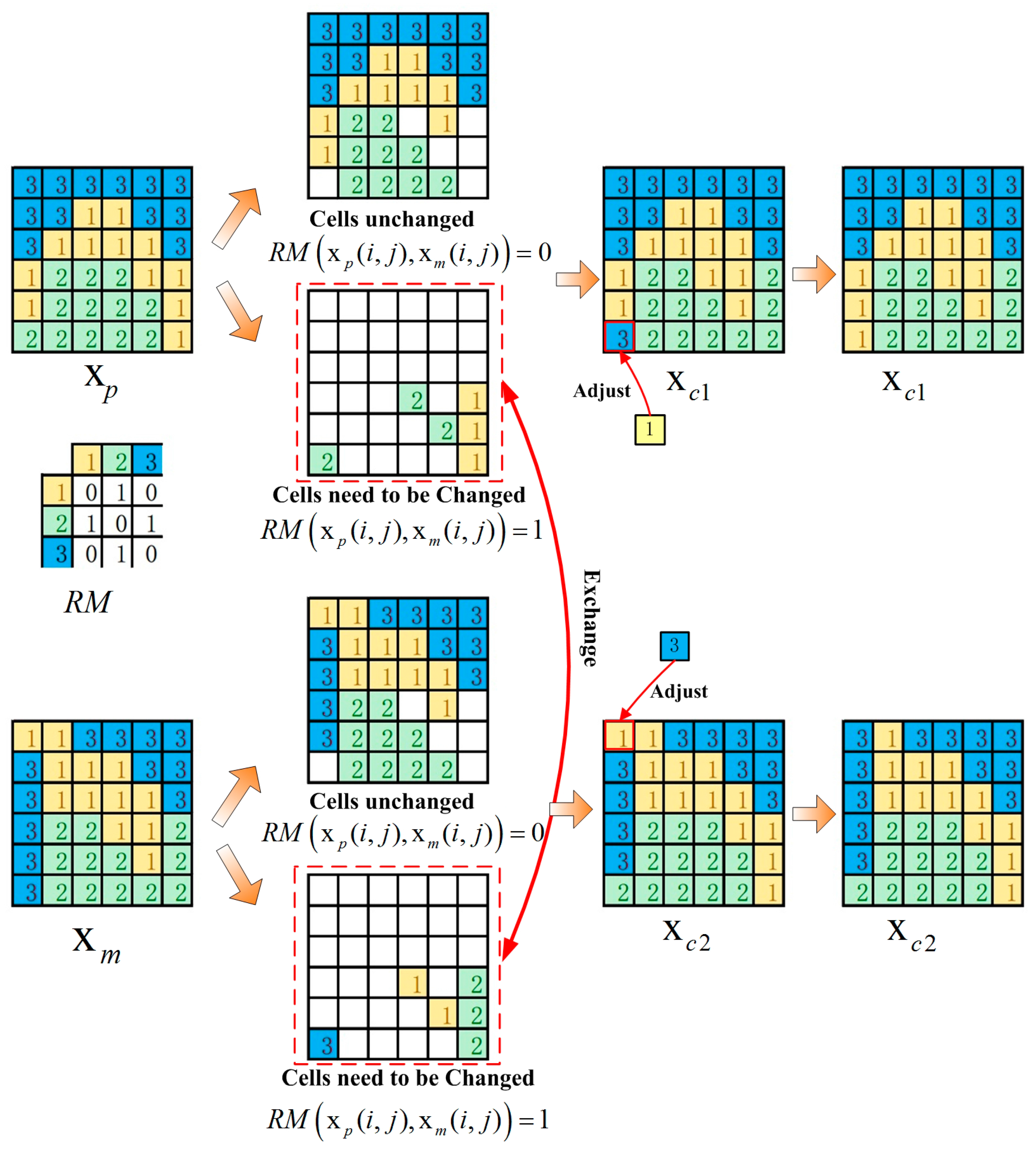
In this study, to promote the diversity of the Pareto-optimal solutions, we generate two new solutions using one crossover operation, and both solutions will take part in the process of Pareto-archive maintenance. The crossover operation is performed according to the following steps, which are also depicted in Figure 5.
First, a solution that is different from the current food source is randomly selected, and these two solutions are duplicated as parent solutions ( X P and X M in Figure 5).
Then, by comparing the parent solutions, a set of raster cells with different land-use types in each parent solution is randomly selected (the two parts of solutions in the two red dotted square frames in Figure 5). Two offspring solutions are constructed by exchanging the selected cells of the two parent solutions. Mathematically, the procedure can be represented by Formula (17):
{ x c 1 ( i , j ) = x p ( i , j ) , x c 2 ( i , j ) = x m ( i , j ) ,   i f   R M ( x p ( i , j ) , x m ( i , j ) ) = 1 x c 1 ( i , j ) = x m ( i , j ) , x c 2 ( i , j ) = x p ( i , j ) ,   e l s e
where R M is a K   ×   K symmetric matrix and K is the number of land-use types that need to be allocated. When k 1 k 2 , R M ( k 1 , k 2 ) is a random number in the set { 0 , 1 } ; otherwise, R M ( k 1 , k 2 ) = 0 . Here, x p ( i , j ) , x m ( i , j ) , x c 1 ( i , j ) and x c 2 ( i , j ) are the land-use types of the two parents’ and two offspring’s solutions, respectively, in cell ( i , j ) .
Finally, after the exchange operation, the land-use types that violate the area restriction must be adjusted by random selection. The two final offspring solutions ( X c 1 and X c 2 in Figure 5) can be obtained.

3.3. Pareto-Archive Maintenance Strategy

Maintaining a Pareto-archive involves combining new solutions with the original Pareto-archive. After judging solution dominance according to the definition of Pareto dominance in Section 2.1, non-dominated solutions will be retained. However, in ABC-MOLA, the maximum capacity of the Pareto archive is predefined. Therefore, if the quantity of non-dominated solutions exceeds the capacity, some inferior solutions with small crowding distance [40] must be deleted.
The crowding distance d x i of a solution x i is the average distance of its two neighboring solutions, which can be calculated by the following steps. First, all solutions in the Pareto-archive are sorted according to the values of a certain objective function. Then, the sum of the Euclidean distances between solution x i and its neighboring solutions x i 1 , x i + 1 in all objective directions is calculated. Finally, d x i is calculated according to Formula (18).
d x i = { , i = 1   or   N m = 2 M 1 | f m ( x i + 1 ) f m ( x i 1 ) | f m max f m min , m = 1 , , M   and   1 < i < N
where M and N are the numbers of objectives and solutions, respectively, i is the sequence number of the reordered solutions and f m max and f m min represent the maximum and minimum values, respectively, of the objective function m for all solutions in the Pareto-archive.
In this study, the solution set of all food sources is also regarded as an archive with maximum capacity S N . The solution-updating strategy for this set in ABC-MOLA is the same as for the Pareto-archive.

3.4. Computational Complexity

In this paper, a solution is of R rows and C columns; the colony size is C S ; the maximum iteration number is M a x i t e r a t i o n s . The mutation proportion is ρ ; the number of objectives is M ; and the quantity of land-use types to be allocated is N l a n d _ t y p e . The ABC-MOLA algorithm’s computational time complexity can be analyzed as follows.
The main parts of the improved neighborhood search strategy’s computational complexity are listed in Table 1, which shows that the overall complexity of neighborhood search is O ( R 2 × C 2 × ρ ) . This neighborhood search complexity is governed by the solution updating procedure of mutation.
Table 2 shows the main procedures involved in the ABC-MOLA algorithm’s computational complexity. It shows that the overall complexity of ABC-MOLA is O ( R 2 × C 2 × ρ × C S × M a x i t e r a t i o n s ) , which is governed by the neighborhood search procedure.

4. Experiments

Two types of experiments were designed for this study. One type of experiment uses simulated data to compare ABC-MOLA with other state-of-the-art algorithms and to validate its effectiveness. Another type of experiment uses real-world data from Jixian county to demonstrate the algorithm’s applicability for practical land-use planning.
The algorithm is coded by Visual C# language. All experiments are carried out on a personal computer (Apple, California, USA) with an Intel (R) Core (TM) i7-4558U 2.8-GHz CPU, 4.00 GB RAM and the Windows 7 operation system.

4.1. Validation with Simulated Data

4.1.1. Simulated Data and Parameter Settings

The simulated data used in this paper come from [28], which requires equal allocation of four land-use types within a region with a size of 36   ×   36 raster cells to maximize spatial compactness and suitability. The area of each land-use type A r e a k ( k = 1 , 2 , 3 , 4 ) occupies 324 raster cells. To reduce the effect of spatial autocorrelation, the suitability of each cell in this region is randomly set to a real number within the range [ 0 , 1 ] , as shown in Figure 6. Here, the maximum and minimum suitability values respectively are S u i t max = 1040.034 and S u i t min = 260.8292 . The maximum and minimum compactness, which are inversely proportional to polygons’ perimeters as explained in Section 2.2, respectively are C o m max = 127.6168 and C o m min = 5184 . Besides, because the factor of spatial autocorrelation can be ignored, the Pareto front should be a curve from point (1,0) to point (0,1) [28].
For the sake of a fair comparison, the value of the mutation proportion is set to the same value as in [28], ρ = 30 % . According to [32], L i m i t = C S × D 2 , where D is the problem dimension. In this study, D = 2 ; thus, L i m i t = C S . The other two parameters are respectively set as C S = 30 and M a x i t e r a t i o n s = 100   s . The effects of these two parameters on the experiment results will be further discussed in Section 5.1. The parameter settings for the ABC-MOLA algorithm are listed in Table 3.

4.1.2. Experiment Results

Based on the parameter settings listed in Section 4.1.1, ABC-MOLA is run 40 times to obtain 40 Pareto fronts. To show the algorithm’s effectiveness, a Pareto front is randomly selected, depicted and compared with the results of AIS-MOLA [28] and PSA-MOLA [3] in Figure 7. In addition, to demonstrate ABC-MOLA’s stability, the solutions with the minimum or maximum compactness and compactness nearest to 0.4, 0.6 and 0.8 are labeled as A, B, C, D and E as depicted in Figure 7 and listed in Table 4.
As Figure 7 shows, ABC-MOLA’s Pareto front totally dominates the Pareto fronts of AIS-MOLA and PSA-MOLA. This means that the optimal solutions obtained by ABC-MOLA are closer to the real Pareto front, which should be a curve from point (1,0) to point (0,1) [28]. This is mainly because the improved mutation and crossover strategies can effectively enhance the performance of the algorithm while seeking for optimal solutions, which will be discussed in Section 5.2. Moreover, the five sets of 40 optimal solutions’ distributions in objective space are very compact, as shown by the small standard deviation value in Table 4. This value is sufficient to demonstrate the stability of the algorithm in acquiring Pareto fronts.
Moreover, five sets of solutions’ spatial patterns, whose positions in ABC-MOLA’s Pareto fronts are close to the five labeled points in Figure 7, are shown in Figure 8. In each set, there are three randomly-selected solutions’ spatial patterns are depicted. The solutions near the point A have the largest value of compactness; thus, the land-use with the same type clusters together to show the best aggregation. Contrarily, the solutions near the point E have the largest value of suitability, but smallest value of compactness; thus, the distributions of land-use types are discrete. Meanwhile, because the spatial autocorrelation factor of this simulated data can be ignored, the spatial patterns of solutions in the same set are different.
Besides, ABC-MOLA requires only 100 s to find this Pareto front, far less than the 164 s of computing time required by AIS-MOLA or the 3958 s required by PSA-MOLA [28], showing that the optimization efficiency of ABC-MOLA is greatly improved. Note that because a different computing environment was used in [28], it may be premature to conclude that ABC-MOLA’s efficiency is better than AIS-MOLA’s, but it is certain that its high calculation efficiency has proven its capacity to solve land-use allocation problems over large areas.

4.2. Application to Real-World Data

4.2.1. Experiment Data

In this article, we choose Jixian county, which is located in the north of Tianjin, China, as a real-world example to execute the multiple objective land-use optimization for its high urbanization rate and long-term development demand. The land-use map has a ground resolution of 150 × 150 m in 2010 (shown in Figure 9), which can be obtained by resampling and classification of Landsat 8 satellite images. It mainly contains five land-use types, built-up land, farm land, forest land, unused land and wetland. Meanwhile, according to local experts’ knowledge [33], the land-use suitability of farm land, forest land and built-up land can be generated, which are shown in Figure 10.
Assuming that the wetland area remains the same, based on the general land-use plan, the areas of allocable built-up land ( A r e a 1 ), farm land ( A r e a 2 ), forest land ( A r e a 3 ) and unused land ( A r e a 4 ) in 2020 can be approximately converted to 12,993, 21,317, 27,995 and 2,367 raster cells. Meanwhile, the main variables in terms of the land-use allocation model are S u i t max = 55,177.17 , S u i t min = 1334.6556 , C o m max = 937.13 and C o m min = 279,544 .
Besides, because of these 64,672 allocable cells and four allocable land-use types, there are 464,672 candidate solutions. It is impossible to find the best solution in a reasonable time among such a mighty search space. Obviously, the experiment can clearly show the complexity of multi-objective optimization while dealing with real-world land-use planning problems.

4.2.2. Experiment Results

The parameter settings of C S , L i m i t and ρ are the same as those used in Section 4.1, and the convergence condition is set to M a x i t e r a t i o n s = 6000   s . After eight runs of ABC-MOLA, eight sets of Pareto fronts are obtained.
Six solutions in each Pareto front with the minimum or maximum compactness, or compactness nearest to 0.88, 0.90, 0.92 and 0.94, were extracted and are depicted by different colors in Figure 11, while their average values and standard deviations are listed in Table 5. The figure and the statistics in the table clearly show that the solutions in each set are distributed in a relatively compact way with small standard deviations. Together, these effectively illustrate ABC-MOLA’s stability when solving real-world land-use allocation problems.
Two randomly-selected Pareto fronts of ABC-MOLA and AIS-MOLA [28] are compared in Figure 12. The one result with the best objective function value after ten times of calculation of the ABC algorithm for single objective land-use allocation, ABC-SOLA [33], which considers the same two objective functions as in this article, compactness and suitability, is also presented in Figure 12. As shown, all the solutions obtained by ABC-MOLA totally dominate those found by AIS-MOLA, indicating that the Pareto front obtained by ABC-MOLA is of better quality than that obtained by AIS-MOLA. The result of ABC-SOLA is just one solution of relative low quality near the Pareto front of ABC-MOLA. Moreover, because the land-use suitability in the real world has a higher spatial autocorrelation than the simulated data shown in Figure 12, the Pareto front is distributed over a relatively narrow range in objective space.
The corresponding spatial patterns of the four labeled solutions in the ABC-MOLA Pareto front and one solution of ABC-SOLA are shown in Figure 13. The five solutions’ land-use conversion from 2010–2020 are shown in Figure 14.
From Figure 13, we can see that Solution A has the greatest spatial compactness, and thus, many aggregated patches emerged in its spatial-pattern map. In contrast, Solution D owns the highest land-use suitability and the lowest compactness; thus, its land-use allocation spatial pattern is the most discrete. Compared to Solution A, Solution B has a more obvious increase in suitability, while suffering only a slight decrease in spatial compactness. Moreover, compared to Solution D, Solution C has higher spatial compactness, but suffers from only a small reduction in suitability. Therefore, in practice, Solutions B and C are preferable for selection as a final urban-planning solution compared to Solutions A and D. This analysis highlights the significance of multi-objective optimization. When dealing with a multi-objective problem, simply converting it into a single-objective problem makes it difficult for decision-makers to observe the large potential losses in objectives resulting from seeking a tiny improvement in one objective. However, using ABC-MOLA can be of great help in allowing decision-makers to analyze the complex tradeoffs among different optimization objectives, and it can provide better-quality solutions for making a final decision.
From Figure 14, several major changes can be observed in all solutions: (1) a large amount of cells donated as farmland in central county are changed into built-up land to satisfy its demand of urbanization; (2) in the northern mountains and southern Jixian, some originally scattered built-up land is respectively transformed into forest and farmland to achieve better compactness; (3) considering the influence of both compactness and suitability, massive unutilized lands in the northern county are converted to forest land, and farmland in the central and southern area are changed into forest land. Besides, it is worth noting that in Solution A, it is compactness, rather than suitability, that is especially considered, so there are a few farmlands are converted to unused land to obtain the largest spatial aggregation, which is not reasonable in practice. Therefore, Solution A should not be a good choice for final decision-making.

5. Discussion

5.1. Sensitivity Analyses

Colony size C S and iteration number M a x i t e r a t i o n s are two important parameters of ABC-MOLA that directly influence the quality of the Pareto front. In this section, we analyze ABC-MOLA’s sensitivity to these two parameters and demonstrate its stability while optimizing land-use allocation.

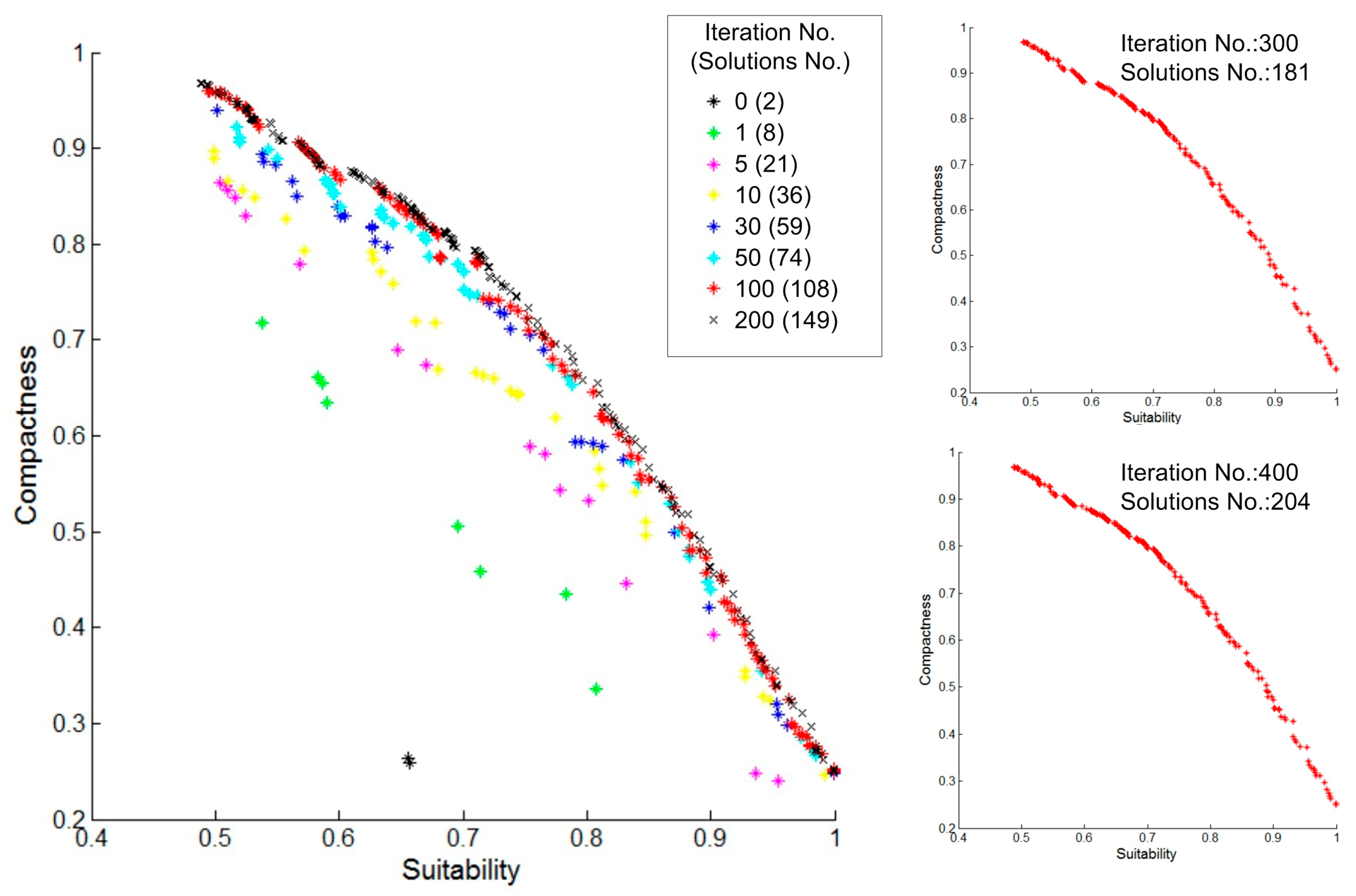
5.1.1. Impact of Iteration Number

A proper number of iteration helps ensure that an optimal solution can be obtained in a reasonable time. Too much iteration prolongs the computation time, while too little prevents a set of optimal solutions from being achieved. To investigate this impact, the spatial distribution of non-dominant solutions in objective space with different numbers of iterations can be recorded with the simulated data under the condition of C S = 30 .
From the results shown in Figure 15, it is evident that at the beginning of the algorithm, non-dominated solutions move quickly towards ideal solutions. By 50 iterations, the curve of the Pareto front is preliminarily formed. By approximately 100 iterations (approximately 25 s of execution time), the shape of the Pareto front tends to be stable. As the calculation continues, the number of non-dominated solutions in the Pareto-optimal solution set increases, and the newly-added solutions simply fine-tune and increase the density of the Pareto front. Therefore, we can conclude that setting the parameter M a x i t e r a t i o n s to a large value (for example, in the experiment, the iteration time is longer than 25 s or, equivalently, extending the number of iterations past 100) has little impact on the formation of the Pareto front.

5.1.2. Impact of Colony Size

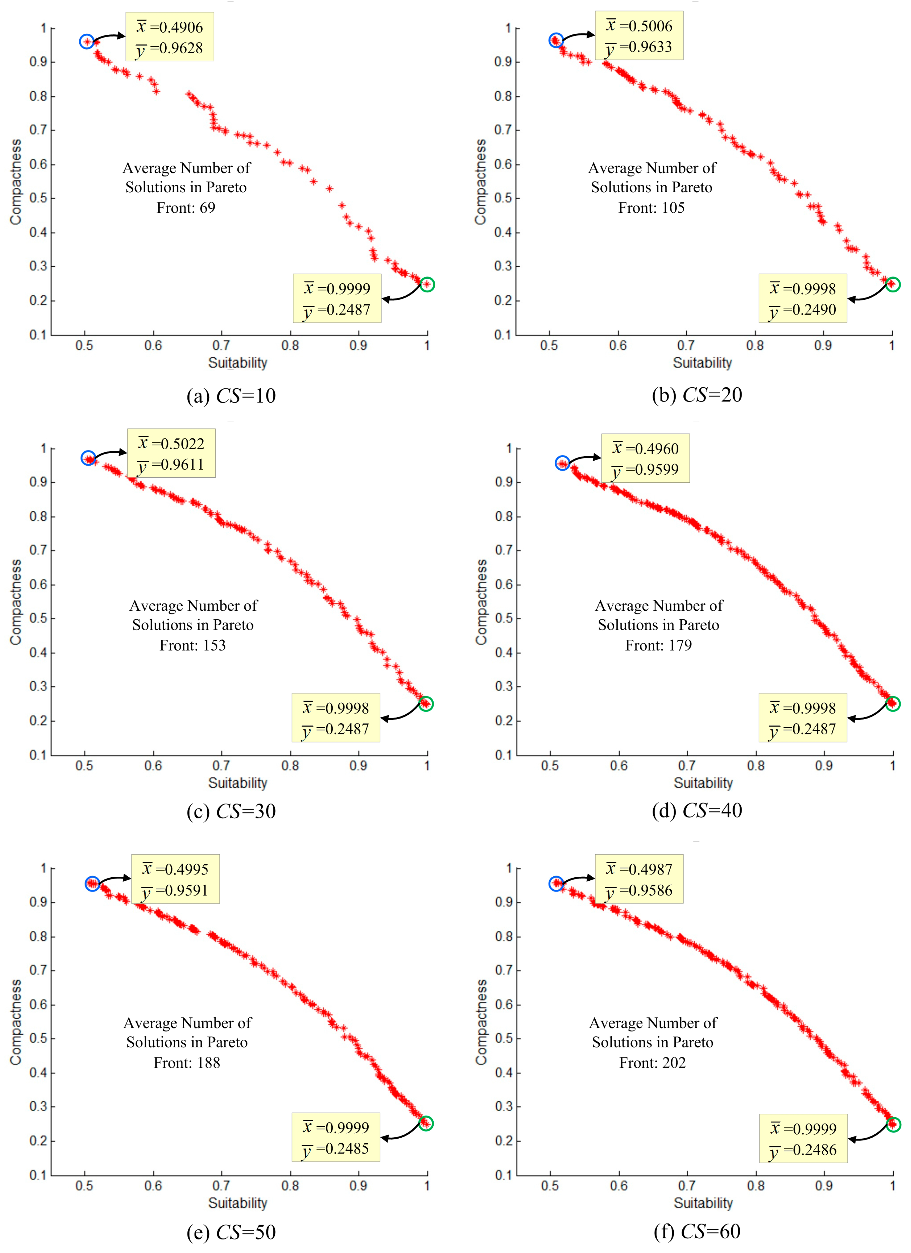
Colony size determines the quantity of solutions in each iteration. Within a certain iteration time, different Pareto fronts of different qualities can be obtained using different colony sizes. To assess this impact, six sets of calculations with different colony population sizes ( C S = 10 , 20 , 30 , 40 , 50 , 60 ) were conducted with simulated data by fixing M a x i t e r a t i o n s = 100   s . Each set is calculated ten times.
The results (Figure 16) indicate that the non-dominated solutions obtained by ABC-MOLA are limited in quantity and cannot form a continuous Pareto-front curve when C S is too small (for example, when C S = 10 , 20 in this experiment). However, as the size of the colony population C S increases, the number of Pareto-optimal solutions obtained in a certain time rises dramatically, and the curves of the Pareto front, which maintain very similar spatial distributions in objective space, tend to be continuous and smooth. Therefore, the value of C S has a small impact on the formation of the Pareto front when its value is relatively large (for example, when C S 30 in this experiment).

5.2. Effectiveness of the Improvements

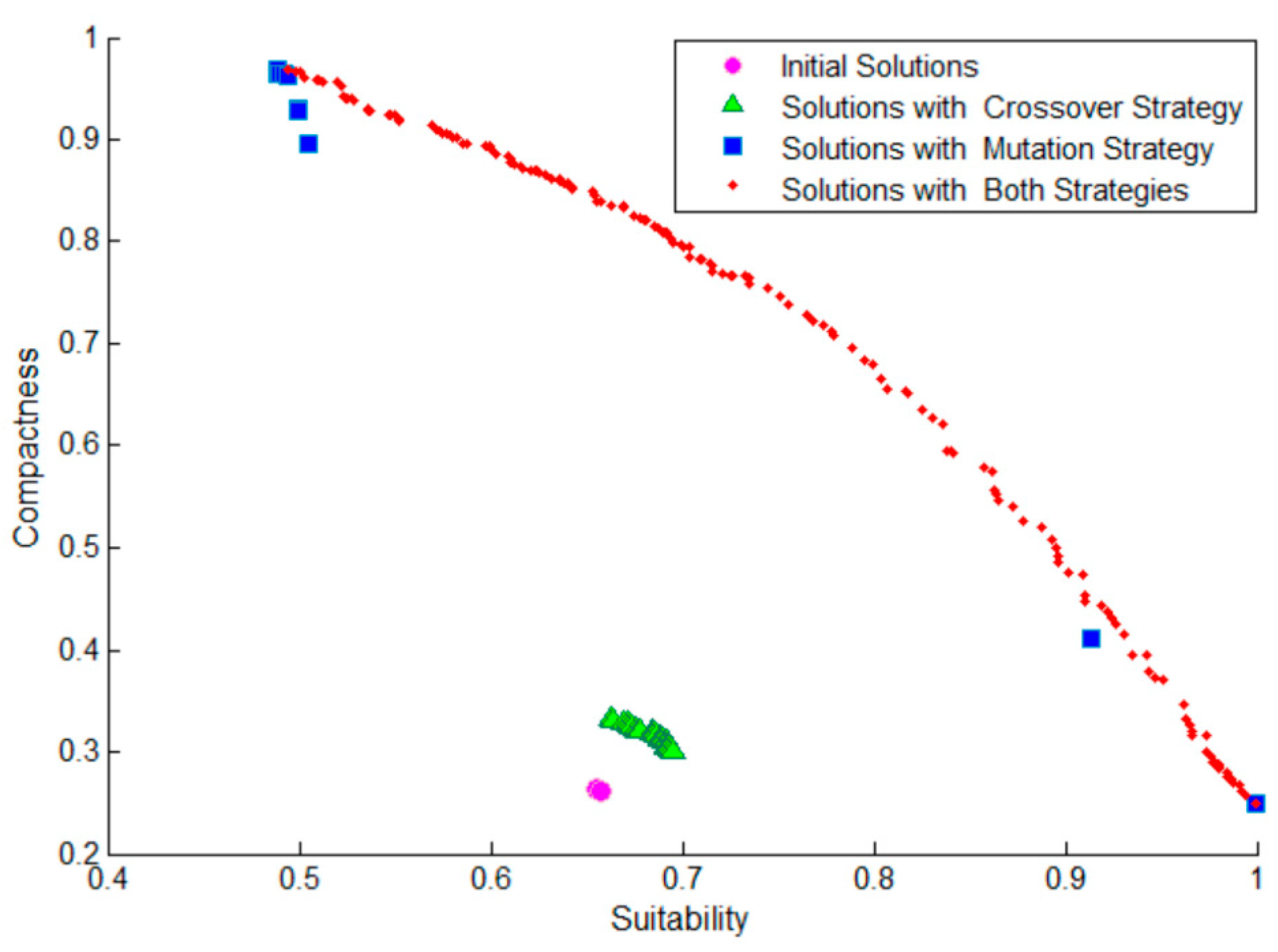
5.2.1. Performance of Improved Search Strategies

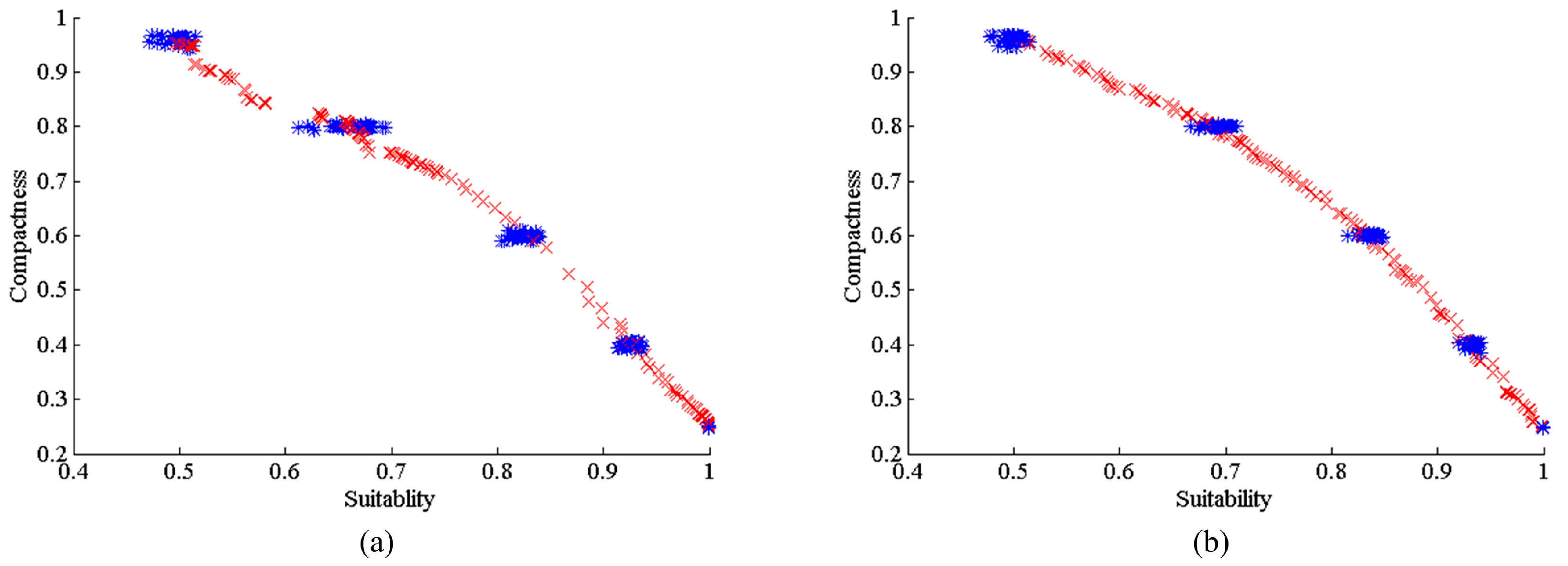
To implement the analysis of neighborhood search strategies, three combinations of neighborhood search strategies were tested: (1) the crossover operator only; (2) the mutation operator only; and (3) a combination of both crossover and mutation operators. The experimental results are shown in Figure 17. The results reveal that after 100 iterations, when only the crossover operator is applied, a continuous and dense Pareto front can still be formed (the green triangle solutions), but with small coverage. In contrast, when only the mutation operator is used, the obtained Pareto front (the blue rectangle solutions) includes some high-quality solutions around its two end vertices, but few in between, indicating poor diversity and uniformity in the spatial distribution. However, when both the crossover and mutation operators are combined, a continuous Pareto-front curve (the red dot solutions) with a uniform distribution and wide coverage is formed in the objective space.
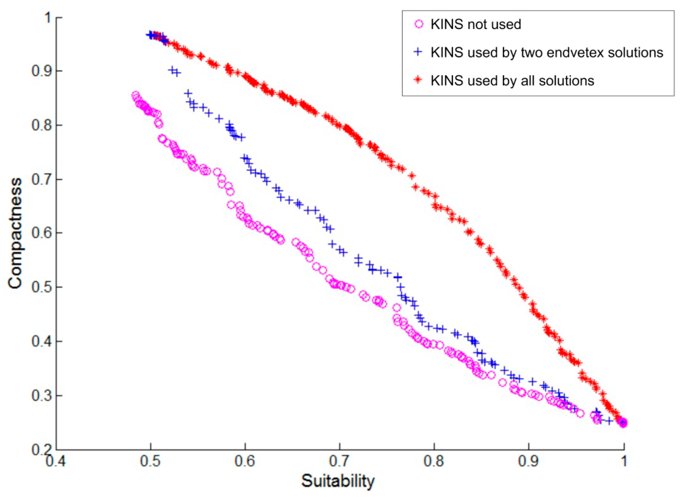
In addition, the KINS strategy was used in each new solution’s generation by neighborhood search in ABC-MOLA. To prove this method’s effectiveness, three comparison experiments based on the search, crossover and mutation operations have been carried out: (1) KINS is not used; (2) KINS is used only by the two end vertex solutions (similar to the strategy used in PSA-MOLA) [3]; and (3) KINS is used by all solutions. The results are shown in Figure 18. The results show that the Pareto front obtained in the first experiment has the lowest quality and is totally dominated by the other two results. The second experiment’s solutions are of similarly high quality to the third experiment’s solutions around the two end vertices of the Pareto front. However, between them, the second experiment’s solutions are totally dominated by the third experiment’s solutions. Obviously, the result of the third experiment has a better Pareto front than the others.

5.2.2. Performance of the ABC Algorithms

The proposed neighborhood search strategies (described in Section 3.2) can be used not only by ABC, but also by many other heuristic algorithms. Here, the artificial immune system (AIS) is coupled with the improved search strategies and compared with the ABC-MOLA algorithm proposed in this paper.
The result (Figure 19) shows that AIS achieves relatively good optimal results while using these search strategies; even better than the AIS-MOLA algorithm proposed by Huang et al. (2013). This effectively validates the portability of these strategies. However, even though the Pareto fronts obtained by AIS are very similar to ABC, they are still inferior to those obtained by ABC, regardless of the uniform distribution of the solutions or the smoothness of the Pareto front curves.

5.3. Potential Use of the Approach

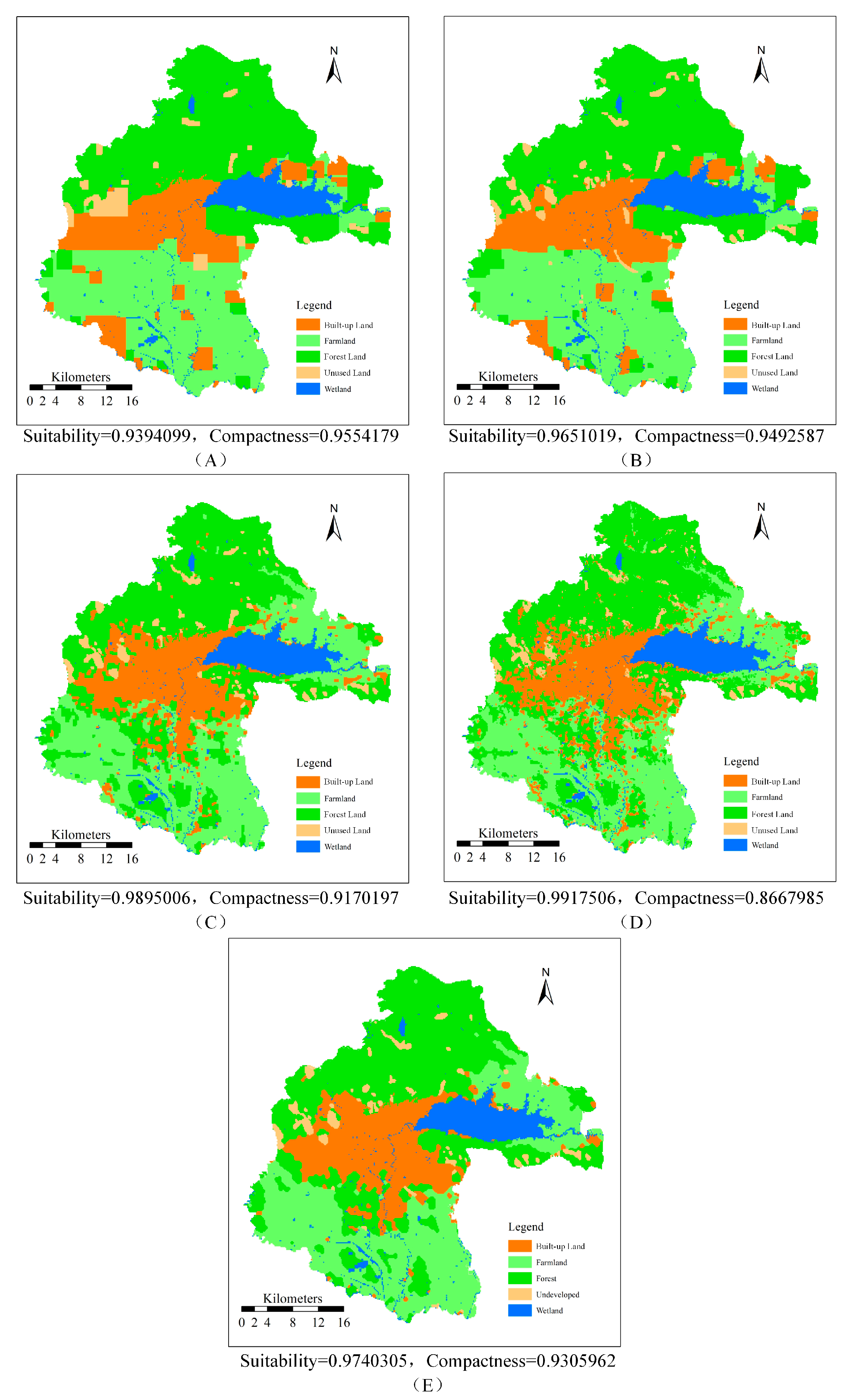
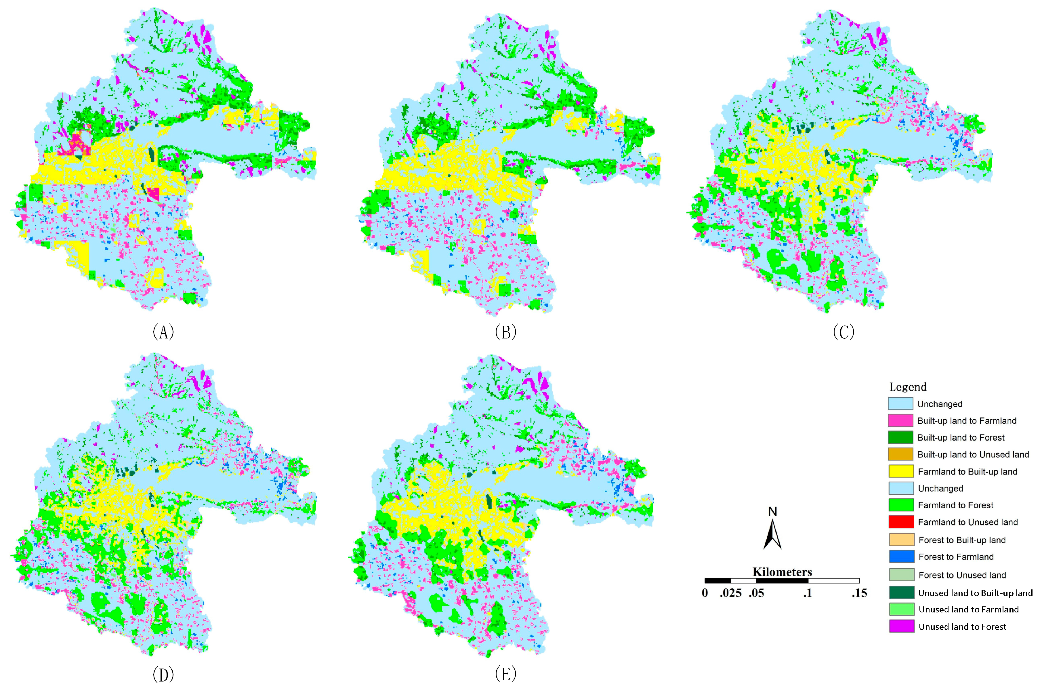
The Pareto front solutions obtained by the proposed approach can be helpful for real regional planning. They can provide a set of optimal solutions for decision-makers, who can choose one solution as the final decision according to their real demands and planning preference. Furthermore, according to the Pareto front solutions’ distribution in objective space, decision-makers can quantitatively analyze one objective function’s reduction while improving the other objective functions, which could be a useful evaluation basis for final decision-making.
Besides, there are two potential uses for the approach presented in this paper. First, from the algorithmic point view, the proposed approach could theoretically be extended to handle problems with three or more objectives. From this perspective, most of the algorithm’s procedures, such as solution initialization, Pareto-archive maintenance and crossover manipulation, are extraneous to the quantity of the objectives. Only the method of determining the weight vector while using the weighted sum strategy in the mutation operation would need some improvement when processed in three or higher dimensions.
Second, from the application perspective, the proposed approach can be used to solve other MOLA problems with different objective functions. Moreover, the proposed approach could also potentially be used in other multi-objective spatial optimization problems in discrete domains—for example, zoning protected ecological areas or selecting facility locations—because these applications exhibit a high degree of similarity to MOLA in terms of problem modeling, solution representation and spatial search requirements.

5.4. Potential Limitations and Challenges

In the mutation strategy, weighted sum, the most commonly-used compromising programming technology, is adopted to evaluate two solutions’ dominance, which is efficient in seeking solutions in the convex part of Pareto front, but deficient in the concave region. Actually, the KINS proposed in this paper can be effectively coupled with the other compromising programming technology, such as weighted Tchebycheff distance, to improve its computation performance while exploring the non-convex solutions of Pareto front.
Besides, as analyzed in Section 3.4, the algorithm’s computational complexity is the second power of the data scale. As the data scale increases in practical application, the computation time will grow dramatically. Therefore, how to solve a MOLA problem for a large area within a reasonable time is quite challenging.

5.5. Contributions

Based on Pareto theory, this paper proposed an improved ABC for MOLA, which aims to provide a set of optimal solutions for decision-makers. For the first time, this paper introduced an improved Pareto-ABC algorithm, an effective method for optimization, to solve MOLA problems and obtain satisfying solutions. ABC-MOLA could be a good way to provide decision-makers with high-quality optimal solutions. Moreover, this paper proposed a strategy that couples auxiliary knowledge of natural geography and spatial structure with the generation of all new solutions, which effectively improved the optimization performance. This strategy can be applied by many other heuristic algorithms to achieve better results. Therefore, the ABC-MOLA algorithm proposed in this paper is a beneficial and useful complement to MOLA optimization.

6. Conclusions and Future Work

The purpose of this study was to develop ABC as a new method that uses a knowledge-informed neighborhood search strategy to improve the quality of Pareto-optimal solutions for MOLA. Different from ABC for SOLA [33] that obtains only one optimal solution under the condition of a set of predefined weights for different objectives, ABC-MOLA is able to get multiple non-dominated solutions. Similar to the main differences existing between ABC for MOOP and SOOP presented in Section 2.3, in ABC-MOLA, different strategies for guiding the bees’ search directions in solution space and for updating solutions both locally and globally have been specifically designed.
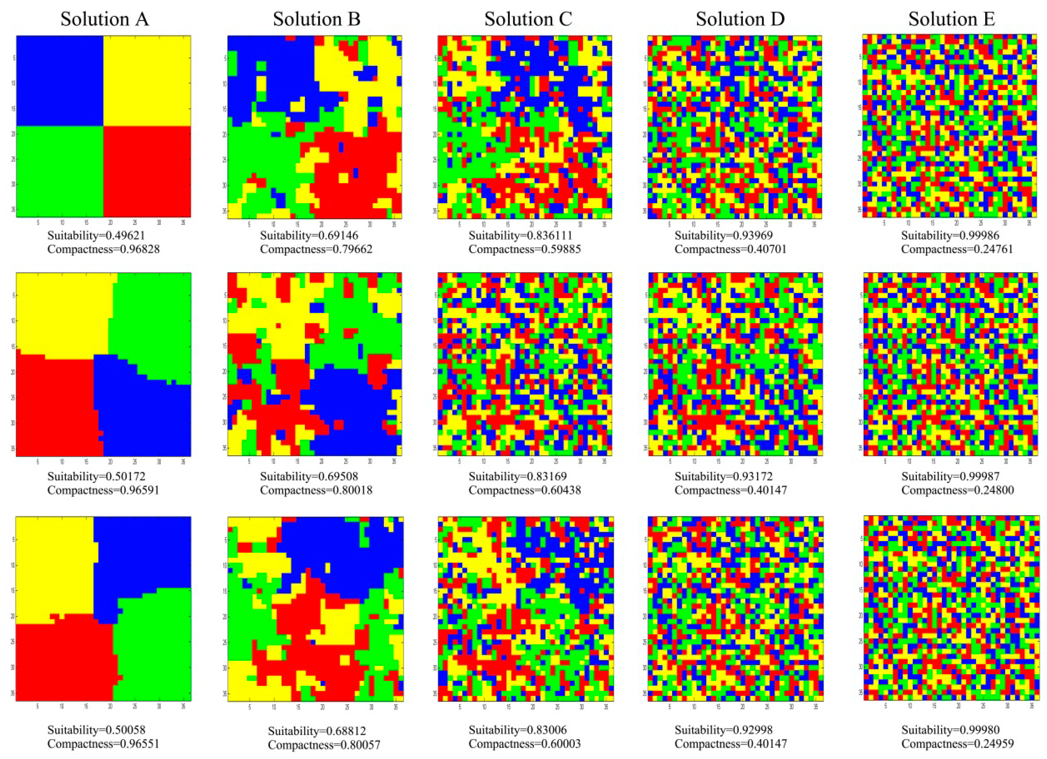
To validate the algorithm’s effectiveness, we treat the land-use allocation problem as a multi-objective spatial-combination optimization problem based on two-dimensional raster data, in which each land-use type’s area is maintained and two commonly-used objective functions, suitability and compactness, are maximized. In a series of comparison experiments, ABC-MOLA shows better optimization ability than other state-of-the-art algorithms and demonstrates good suitability for solving grid-represented land-use allocation problems in large areas.
Notably, the proposed ABC-MOLA is used to solve a land-use allocation problem with only two objectives in this paper. In the future, we plan to make further improvements to ABC-MOLA so it will be able to solve problems with three or more objectives, which are still intractable. Moreover, when solving problems that involve large areas, the calculation time required for ABC-MOLA increases dramatically. Therefore, we plan to further improve ABC-MOLA’s computational efficiency for multi-objective land-use allocation.

Acknowledgments

This study was supported by the Open Research Fund of Key Laboratory of Digital Earth Science, Institute of Remote Sensing and Digital Earth, Chinese Academy of Sciences (2015LDE002) and the Director Foundation of Institute of Remote Sensing and Digital Earth, Chinese Academy of Sciences (Y6SJ2300CX).

Author Contributions

Lina Yang and Tianhe Chi proposed the original idea of this paper; Axing Zhu improved the idea of the paper; Lina Yang conceived the methodology and designed the experiments; Jing Shao performed the experiments; Lina Yang analyzed the results and wrote the paper.

Conflicts of Interest

The authors declare no conflict of interests.

References

  1. Li, X.; Liu, X. Embedding sustainable development strategies in agent-based models for use as a planning tool. Int. J. Geogr. Inf. Sci. 2008, 22, 21–45. [Google Scholar] [CrossRef]
  2. Li, X.; Yeh, A. Integration of genetic algorithms and gis for optimal location search. Int. J. Geogr. Inf. Sci. 2005, 19, 581–601. [Google Scholar] [CrossRef]
  3. Duh, J.; Brown, D.G. Knowledge-informed pareto simulated annealing for multi-objective spatial allocation. Comput. Environ. Urban Syst. 2007, 31, 253–281. [Google Scholar] [CrossRef]
  4. Li, X.; Lao, C.; Liu, X.; Chen, Y. Coupling urban cellular automata with ant colony optimization for zoning protected natural areas under a changing landscape. Int. J. Geogr. Inf. Sci. 2011, 25, 575–593. [Google Scholar] [CrossRef]
  5. Tong, D.; Murray, A.T. Spatial optimization in geography. Ann. Assoc. Am. Geogr. 2012, 102, 1290–1309. [Google Scholar] [CrossRef]
  6. Huang, B.; Zhang, W. Sustainable land-use planning for a downtown lake area in central china: Multiobjective optimization approach aided by urban growth modeling. J. Urban Plan. Dev. 2014, 140, 1–12. [Google Scholar] [CrossRef]
  7. Cao, K.; Batty, M.; Huang, B.; Liu, Y.; Yu, L.; Chen, J. Spatial multi-objective land use optimization: Extensions to the non-dominated sorting genetic algorithm-ii. Int. J. Geogr. Inf. Sci. 2011, 25, 1949–1969. [Google Scholar] [CrossRef]
  8. Brookes, C.J. A genetic algorithm for designing optimal patch configurations in gis. Int. J. Geogr. Inf. Sci. 2001, 15, 539–559. [Google Scholar] [CrossRef]
  9. Ligmann Zielinska, A.; Church, R.L.; Jankowski, P. Spatial optimization as a generative technique for sustainable multiobjective land-use allocation. Int. J. Geogr. Inf. Sci. 2008, 22, 601–622. [Google Scholar] [CrossRef]
  10. Church, R.L. Location modelling and gis. In Geographical Information Systems; Wiley: Hoboken, NJ, USA, 1999; pp. 293–303. [Google Scholar]
  11. Stewart, T.J.; Janssen, R.; van Herwijnen, M. A genetic algorithm approach to multiobjective land use planning. Comput. Oper. Res. 2004, 31, 2293–2313. [Google Scholar] [CrossRef]
  12. Eastman, J.R.; Jin, W.; Keym, P.; Toledano, J. Raster procedures for multi-creteria/multi-objective decisions. Photogramm. Eng. Rem. S 1995, 61, 539–547. [Google Scholar]
  13. Zadeh, L. Optimality and non-scalar-valued performance criteria. IEEE Trans. Automat. Contr. 1963, 8, 59–60. [Google Scholar] [CrossRef]
  14. Charnes, A.; Cooper, W.W.; Ferguson, R.O. Optimal estimation of executive compensation by linear programming. Manag. Sci. 1955, 1, 138–151. [Google Scholar] [CrossRef]
  15. Haimes, Y.Y.; Lasdon, L.S.; Wismer, D.A. On a bicriterion formulation of the problems of integrated system identification and system optimization. IEEE Trans. Syst. Man Cybern. 1971, 1, 296–297. [Google Scholar]
  16. Miettinen, K. Nonlinear Multiobjective Optimization; Kluwer Academic: Boston, MA, USA, 1999. [Google Scholar]
  17. Huang, B.; Fery, P.; Xue, L.; Wang, Y. Seeking the pareto front for multiobjective spatial optimization problems. Int. J. Geogr. Inf. Sci. 2008, 5, 507–526. [Google Scholar] [CrossRef]
  18. Roberts, S.A.A.H. Evolutionary multi-objective optimization for landscape system design. J. Geogr. Syst. 2011, 13, 299–326. [Google Scholar] [CrossRef]
  19. Srinivas, N.; Deb, K. Multiobjective optimization using nondominated sorting in genetic algorithms. Evol. Comput. 1994, 2, 221–248. [Google Scholar] [CrossRef]
  20. Deb, K.; Pratap, A.; Agarwal, S.; Meyarivan, T. A fast and elitist multiobjective genetic algorithm: Nsga-ii. IEEE Trans. Evolut. Comput. 2002, 6, 182–197. [Google Scholar] [CrossRef]
  21. Czyzżak, P.; Jaszkiewicz, A. Pareto Simulated Annealing—A Metaheuristic Technique for Multiple-Objective Combinatorial Optimization; John Wiley & Sons, Ltd.: Hoboken, NJ, USA, 1998; Volume 7, pp. 34–47. [Google Scholar]
  22. Zitzler, E.; Thiele, L. Multiobjective evolutionary algorithms: A comparative case study and the strength pareto approach. IEEE Trans. Evolut. Comput. 1999, 3, 257–271. [Google Scholar] [CrossRef]
  23. Zitzler, E.; Laumanns, M.; Thiele, L. Spea2: Improving the Strength Pareto Evolutionary Algorithm; Computer Engineering and Networks Laboratory (TIK); Department of Electrical Engineering, Swiss Federal Institute of Technology (ETH): Zurich, Switzerland, 2001. [Google Scholar]
  24. Coello, C.A.C.; Pulido, G.T.; Lechuga, M.S. Handling multiple objectives with particle swarm optimization. IEEE Trans. Evolut. Comput. 2004, 8, 256–279. [Google Scholar] [CrossRef]
  25. Coello, C.A.C.; Cortes, N.C. Solving multiobjective optimization problems using an artificial immune system. Genet. Program. Evol. Mach. 2005, 6, 163–190. [Google Scholar] [CrossRef]
  26. David, A.; Bennett, N.X.M.P. Exploring the geographic consequences of public policies using evolutionary algorithms. Ann. Assoc. Am. Geogr. 2004, 94, 827–847. [Google Scholar]
  27. Matthews, K.B.; Craw, S.; Elder, S.; Sibbald, A.R.; MacKenzie, I. Applying Genetic Algorithms to Multi-Objective Land Use Planning. In Proceedings of the Genetic and Evolutionary Computation Conference, Las Vegas, NV, USA, 10–12 July 2001; pp. 613–620. [Google Scholar]
  28. Huang, K.; Liu, X.; Li, X.; Liang, J.; He, S. An improved artificial immune system for seeking the pareto front of land-use allocation problem in large areas. Int. J. Geogr. Inf. Sci. 2013, 27, 922–946. [Google Scholar] [CrossRef]
  29. Chen, W.; Wiecek, M.M.; Zhang, J. Quality utility—A compromise programming approach to robust design. J. Mech. Design. 1999, 121, 179–187. [Google Scholar] [CrossRef]
  30. Andre, J.; Siarry, P.; Dognon, T. An improvement of the standard genetic algorithm fighting premature convergence in continuous optimization. Adv. Eng. Softw. 2001, 32, 49–60. [Google Scholar] [CrossRef]
  31. Karaboga, D.; Basturk, B. On the performance of artificial bee colony (abc) algorithm. Appl. Soft Comput. 2008, 8, 687–697. [Google Scholar] [CrossRef]
  32. Karaboga, D.; Akay, B. A comparative study of artificial bee colony algorithm. Appl. Math. Comput. 2009, 214, 108–132. [Google Scholar] [CrossRef]
  33. Yang, L.; Sun, X.; Peng, L.; Shao, J.; Chi, T. An improved artificial bee colony algorithm for optimal land-use allocation. Int. J. Geogr. Inf. Sci. 2015, 29, 1470–1489. [Google Scholar] [CrossRef]
  34. Karaboga, D.; Gorkemli, B.; Ozturk, C.; Karaboga, N. A comprehensive survey: artificial bee colony (abc) algorithm and applications. Artif. Intell. Rev. 2014, 42, 21–57. [Google Scholar] [CrossRef]
  35. Omkar, S.N.; Senthilnath, J.; Khandelwal, R.; Naik, G.N.; Gopalakrishnan, S. Artificial bee colony (abc) for multi-objective design optimization of composite structures. Appl. Soft Comput. 2011, 11, 489–499. [Google Scholar] [CrossRef]
  36. Li, J.; Pan, Q.; Gao, K. Pareto-based discrete artificial bee colony algorithm for multi-objective flexible job shop scheduling problems. Int. J. Adv. Manuf. Technol. 2011, 55, 1159–1169. [Google Scholar] [CrossRef]
  37. Wang, L.; Zhou, G.; Xu, Y.; Liu, M. An enhanced pareto-based artificial bee colony algorithm for the multi-objective flexible job-shop scheduling. Int. J. Adv. Manuf. Technol. 2012, 60, 1111–1123. [Google Scholar] [CrossRef]
  38. Zou, W.; Zhu, Y.; Chen, H.; Shen, H. A Novel Multi-Objective Optimization Algorithm Based on Artificial Bee Colony: Gecco ’11; ACM: New York, NY, USA, 2011; pp. 103–104. [Google Scholar]
  39. Akbari, R.; Hedayatzadeh, R.; Ziarati, K.; Hassanizadeh, B. A multi-objective artificial bee colony algorithm. Swarm Evol. Comput. 2012, 2, 39–52. [Google Scholar] [CrossRef]
  40. Deb, K.; Agrawal, S.; Pratap, A.; Meyarivan, T. A fast elitist non-dominated sorting genetic algorithm for multi-objective optimization: Nsga-II. In International Conference on Parallel Problem Solving From Nature; Springer: Berlin/Heidelberg, Germany, 2000; pp. 849–858. [Google Scholar]
Figure 1. Pareto solutions.
Ijgi 07 00063 g001
Figure 2. The main procedure of the ABC- multi-objective land-use allocation (MOLA) algorithm.
Ijgi 07 00063 g002
Figure 3. Solution selection in objective space based on the weighted sum technique.
Ijgi 07 00063 g003
Figure 4. The spatial distribution of solutions’ weight vectors in objective space.
Ijgi 07 00063 g004
Figure 5. The crossover operation.
Ijgi 07 00063 g005
Figure 6. Suitability for 4 types of land-use in the hypothetical experiment (adapted from [28]). (a) The suitability of Land-use type 1; (b) The suitability of Land-use type 2; (c) The suitability of Land-use type 3; (d) The suitability of Land-use type 4.
Ijgi 07 00063 g006
Figure 7. Pareto fronts of generated by ABC-MOLA, artificial immune system (AIS)-MOLA and Pareto simulated annealing (PSA)-MOLA. The latter two algorithms’ Pareto fronts are adapted from [28].
Ijgi 07 00063 g007
Figure 8. Corresponding spatial patterns of solutions in three random selected Pareto fronts with their approximate positions labeled in Figure 7.
Ijgi 07 00063 g008
Figure 9. The location and land-use map of Jixian (the land-use data are adapted from [33]).
Ijgi 07 00063 g009
Figure 10. Land-use suitability in the experiment area (the suitability data are adapted from [33]). (a) The suitability of Farm Land; (b) The suitability of Forest Land; (c) The suitability of Built-up Land
Ijgi 07 00063 g010
Figure 11. Distribution of six sets of solutions in Pareto fronts of Pareto-ABC algorithms based on 8 experiment results.
Ijgi 07 00063 g011
Figure 12. The Pareto fronts of ABC-MOLA and AIS-MOLA [28], and ABC-SOLA [33] solution in Jixian land-use optimization.
Ijgi 07 00063 g012
Figure 13. The spatial allocation of the five labelled solutions in Figure 12. (A) The spatial allocation of solution A; (B) The spatial allocation of solution B; (C) The spatial allocation of solution C; (D) The spatial allocation of solution D; (E) The spatial allocation of solution E.
Ijgi 07 00063 g013
Figure 14. The land conversion in Jixian from 2010–2020 of the five labelled solutions in Figure 12. (A) The land conversion of solution A; (B) The land conversion of solution B; (C) The land conversion of solution C; (D) The land conversion of solution D; (E) The land conversion of solution E.
Ijgi 07 00063 g014
Figure 15. Pareto solutions for different numbers of iterations.
Ijgi 07 00063 g015
Figure 16. Results of ABC-MOLA with different C S values. The red dots are the solutions in the Pareto front, and x ¯ and y ¯ are the average values of suitability and compactness, respectively. (a) The Pareto front while C S = 10 ; (b) The Pareto front while C S = 20 ; (c) The Pareto front while C S = 30 ; (d) The Pareto front while C S = 40 ; (e) The Pareto front while C S = 50 ; (f) The Pareto front while C S = 60 .
Ijgi 07 00063 g016
Figure 17. Comparison of different neighborhood search strategies.
Ijgi 07 00063 g017
Figure 18. Comparison of different applications of knowledge-informed neighborhood search (KINS).
Ijgi 07 00063 g018
Figure 19. Pareto solutions’ distribution of ABC and AIS. Two randomly-selected Pareto fronts obtained by AIS (a) and ABC (b) are represented by red crosses. Five solutions in each Pareto front (forty Pareto fronts in total) with the minimum or maximum compactness values—compactness values nearest to 0.4, 0.6 and 0.8—are represented by the blue stars.
Ijgi 07 00063 g019
Table 1. Computational complexity of the improved neighborhood search strategy.
Main StepsComputational Complexity
Mutation: (1) Calculating each land-use unit’s weighted sum of M functions’ increments if a land-use type is allocated O ( R × C × N l a n d _ t y p e × M )
Mutation: (2) Solution selection based on compromising programming O ( R 2 × C 2 × ρ )
Crossover O ( R × C )
Table 2. Computational complexity of ABC-MOLA.
Main StepsComputational Complexity
Solution initialization O ( M × R × C × C S )
Random solution selection O ( C S × M a x i t e r a t i o n s )
Neighborhood search O ( R 2 × C 2 × ρ × C S × M a x i t e r a t i o n s )
Crowding distance calculation O ( M × C S × log ( C S ) × M a x i t e r a t i o n s )
Pareto archive maintenance O ( C S × log ( C S ) × M a x i t e r a t i o n s )
Table 3. The ABC-MOLA parameter values.
ParameterValue
Population size C S 30
Convergence parameter M a x i t e r a t i o n s 100 s
Scout control parameter L i m i t 30
Mutation proportion ρ 30%
Table 4. Statistics of five sets of solutions labeled in the Pareto front of Pareto-ABC algorithms (labeled in Figure 7) based on 40 experiment results.
SuitabilityCompact
Average ValueStandard DeviationAverage ValueStandard Deviation
A0.49880.00860.96050.0061
B0.69270.00990.80000.0019
C0.83680.00690.60010.0024
D0.93270.00450.39990.0041
E0.99980.00000.24870.0008
Table 5. Statistics of the six sets of solutions shown in Figure 11.
SuitabilityCompact
Average ValueStandard DeviationAverage ValueStandard Deviation
Set 10.94430.00330.95360.0017
Set 20.97600.00210.94050.0010
Set 30.98860.00100.92060.0019
Set 40.98970.00040.90300.0117
Set 50.99040.00070.87870.0052
Set 60.99170.00000.86690.0001

