Article

Single-Frequency Kinematic Performance Comparison between Galileo, GPS, and GLONASS Satellite Positioning Systems Using an MMS-Generated Trajectory as a Reference: Preliminary Results

1
DICATECh—Politecnico di Bari, Via Orabona 4, 70125 Bari, Italy
2
GeoSNav Lab, Università degli Studi di Trieste, via Valerio 6/2, 34127 Trieste, Italy
*
Author to whom correspondence should be addressed.
ISPRS Int. J. Geo-Inf. 2018, 7(3), 122; https://doi.org/10.3390/ijgi7030122
Submission received: 24 January 2018 / Revised: 27 February 2018 / Accepted: 14 March 2018 / Published: 18 March 2018

Abstract

:
The initial Galileo satellite positioning services, started on December 15, 2016, became available with a formal announcement by the European Commission. This first step toward the Galileo system Full Operational Capability (FOC) has allowed many researchers to test the new system. The aim of this paper is to illustrate the results and the conclusions of a kinematic test involving a GNSS (Global Navigation Satellite System) multi-constellation receiver able to acquire the Galileo Open Service (OS) signal. The produced outputs were compared to a reference trajectory obtained from a Mobile Mapping System (MMS) implementing integrated high-performance GPS/INS measurements. By exploiting the CUI (command user interface) of the open source library RTKLIB, a reduced operative status was simulated for GPS and GLONASS. Specifically, all the possible operative combinations were tested and, when possible, statistically assessed. This was necessary to offer a fair comparison among the tested constellations. The results, referred to the reference trajectory, show that the new European system is characterized by a better planimetric performance with respect to the other systems, whereas, from an altimetric point of view, the GPS and GLONASS systems perform better.

1. Introduction

The Galileo navigation satellite system is a global positioning European program designed to be completely interoperable with the analogues GPS and GLONASS positioning systems produced by the United States of America (USA) and the Russian Federation. With Galileo, the European Union aims at owning and providing an independent positioning/navigation service under civilian control [1].
The Galileo program is constituted of two macro-phases: the In-Orbit Validation (IOV) phase and the Full Operational Capability (FOC) phase, which is to reach its conclusion in 2020. Specifically, the Galileo system robustness was tested during the IOV by means of two satellites (GIOVE-A and GIOVE-B) and, subsequently, with a reduced constellation of only four satellites (and the related ground infrastructure) with the aim to synchronize the satellites' onboard atomic clocks and to perform a precise orbit tracking. Further details related to the IOV phase can be found in the works of Simsky et al. and Steigenberger et al. [2,3,4,5], while details related to the problems encountered during this phase can be found in [6,7].
The first step toward the FOC phase was the European Commission’s formal announcement of the Galileo Initial Services (December 15, 2016). Once the FOC phase is concluded, the constellation will rely on 24 satellites (and two backup satellites for each orbital plane). In this phase, each satellite will take 14 h to complete its orbit at the altitude of 23,222 km [8]. The whole system is designed to guarantee that at least four satellites are visible from each point on Earth. Indeed, 24 satellites will be equally distributed on three different orbital planes at 56° with respect to the equatorial plane [9]. Further details related to the preliminary analysis of the FOC phase can be found in the novel work of Zaminpardaz S. and Teunissen P.J.G. [10], while a detailed review of the project status (up to 5 July 2016) can be found in [11].
The Galileo system is designed to provide different services. In this paper, the Galileo Open Service (OS) [8] was considered. The Galileo OS is freely available for mass applications of synchronization and positioning. This service does not require any authorization and can be used by anyone equipped with an adequate receiver. The OS provides up to four carrier frequencies: E1 (1575.42 MHz), E5a (1176.45 MHz), E5b (1207.14 MHz), and E6 (1278.75 MHz). Over the past years, many authors have analyzed the outcomes of the Galileo mission in order to produce communications and scientific works. In particular, tests were produced before the IOV phase by using a simulated Galileo signal (e.g., [12,13,14]). During the IOV phase, Odijk et al. [15] proposed a paper describing the results of mixed GPS and GIOVE (Galileo In-Orbit Validation Element) A/B data. They placed emphasis on the equations related to the intersystem solution and found that the GPS and GIOVE data combinations were able to improve the instantaneous ambiguity resolution with regards to the single GPS data. Cai et al. [16] analyzed the Galileo IOV positioning and signal performance by using the four IOV satellites. In their work, they considered the carrier-to-noise density ratio and multipath, and also analyzed the accuracy of the broadcasted ephemeris and IOV Galileo positioning performance. They concluded that the Galileo signal-to-noise ratio density was bigger than that of the GPS and that Galileo signals are characterized by smaller multipath and noise compared to GPS signals. Gaglione et al. [17] proposed a study to demonstrate the improvement, of the Galileo constellation geometry, associated with the addition of two FOC satellites (FOC-FM1 and FOC-FM2). They also considered the pre- and post-orbital shifts of the FOC-FM1 satellite. Gioia et al. [18] focused their work on the accuracy of the IOV measurements. One week of IOV acquisitions were processed to assess the results.
Studies characterized by GPS, GLONASS, BeiDou, Galileo, and QZSS comparisons are also reported in the literature. In particular, Tegedor et al. [19] worked on precise orbit determination and precise point positioning (PPP) with GPS, GLONASS, Galileo, and BeiDou data. In their work, Galileo (IOV) and Beidu PPP were achieved after precise estimation of their orbit and clocks. This was possible thanks to the MGEX (IGS Multi-GNSS Experiment) data and to the data provided by a proprietary network (Fugro). Lou et al. [20] used a multi-GNSS PPP model to evaluate the performance of the proposed model by using the MGEX data. Their analysis was validated with one month of acquisitions from the MGEX network. Multi-GNSS PPP was also the topic of the works proposed by Liu et al. [21], Pan et al. [22], and Afifi et al. [23]. The work of Cai et al. [24] aimed to assess and compare the multipath and receiver noises for GPS, BeiDou, GLONASS, and Galileo data by implementing the zero-baseline approach. Multi-GNSS performance evaluation was also the objective of the study proposed by Pan et al. [25]. Their work focused on the contemporary use of four constellation data and on the implementation of different data combinations. MGEX data were also used in the paper of Guo et al. [26]. In this case, the aim of the work was the assessment of the precise orbits and clocks for Galileo, BeiDou, and QZSS. This was performed by comparing the outcomes of different analysis centers and laser satellite ranging. Galileo data were involved also in real-time multi GNSS applications. Odijk et al. [27] worked on real-time kinematic (RTK) based both on carrier-phase measurements and on pseudorange measurements acquired from the IOV Galileo satellites (already able to transmit navigation data). They tested different combinations considering only the Galileo signals and the combined Galileo and GPS signals and found that the Galileo and GPS combination could lead to an instantaneous ambiguity resolution. Odolinski et al. [28] proposed a multi GNSS single-frequency real-time kinematic study, while Li et al. [29] focused their attention on the real-time multi GNSS precise orbit determination, clock estimation, and positioning. Galileo data were also tested for attitude estimation (e.g., [30,31]) and included in an online service devoted to the validation of multi-GNSS orbits by means of the satellite laser ranging [32]. Lastly, Galileo data were measured for GNSS reflectometry polarimetric acquisitions over boreal forests [33].
Thus far, this paper has shown the rigor with which, in many studies, the Galileo data were tested and assessed, especially in static sessions of measurements. However, to the authors’ knowledge, there are no examples of kinematic trajectory comparisons between the Galileo positioning performance and GPS- and GLONASS-derived trajectories, by using a reference trajectory derived from a precise Mobile Mapping System (MMS) as a benchmark. Specifically, in this paper, we propose a preliminary (and empiric) single-frequency kinematic performance assessment of Galileo, GPS, and GLONASS data acquired by using a Leica GS14 receiver, with reference to a trajectory estimated with MMS equipped with a POS/LV (Position and Orientation System for Land Vehicles), produced by the Applanix corporation. The Applanix system features a filtering system capable of integrating GNSS measurements with an IMU (inertial measurement unit) in order to guarantee a stable, reliable, and repeatable positioning solution for land-based vehicle applications [34] and to ensure better positioning performance with regard to GNSS-only measurements (complementary and surpassing property [35]). The performed trajectory comparisons were produced in such a way as to consider, for the three positioning systems, all the possible combinations (with four, five and six satellites for each considered constellation), by simulating a reduced operability for GPS and GLONASS. In this way, all the real and comparable working conditions, among the three different constellations, were simulated for a real case study. All the positioning solutions (and trajectories) were computed by means of the Free and Open-Source Software (FOSS) RTKLIB. RTKLIB is an open-source program package for standard and precise positioning and consists of a portable program library and several APs (application programs) already used in previous scientific communications [36,37,38,39,40]. It supports: (1) standard and precise positioning algorithms with GPS, GLONASS, Galileo, QZSS, BeiDou, and SBAS; (2) single, DGPS/DGNSS, Kinematic, Static, Moving-Baseline, Fixed, PPP-Kinematic, PPP-Static, and PPP-Fixed positioning modes with GNSS for both real-time and post-processing (further details can be found in [41]).
The final results of the performed experiment were statistically assessed and showed a better Galileo planimetric performance while, from an altimetric point of view, the GPS and GLONASS systems performed better.

2. Materials and Methods

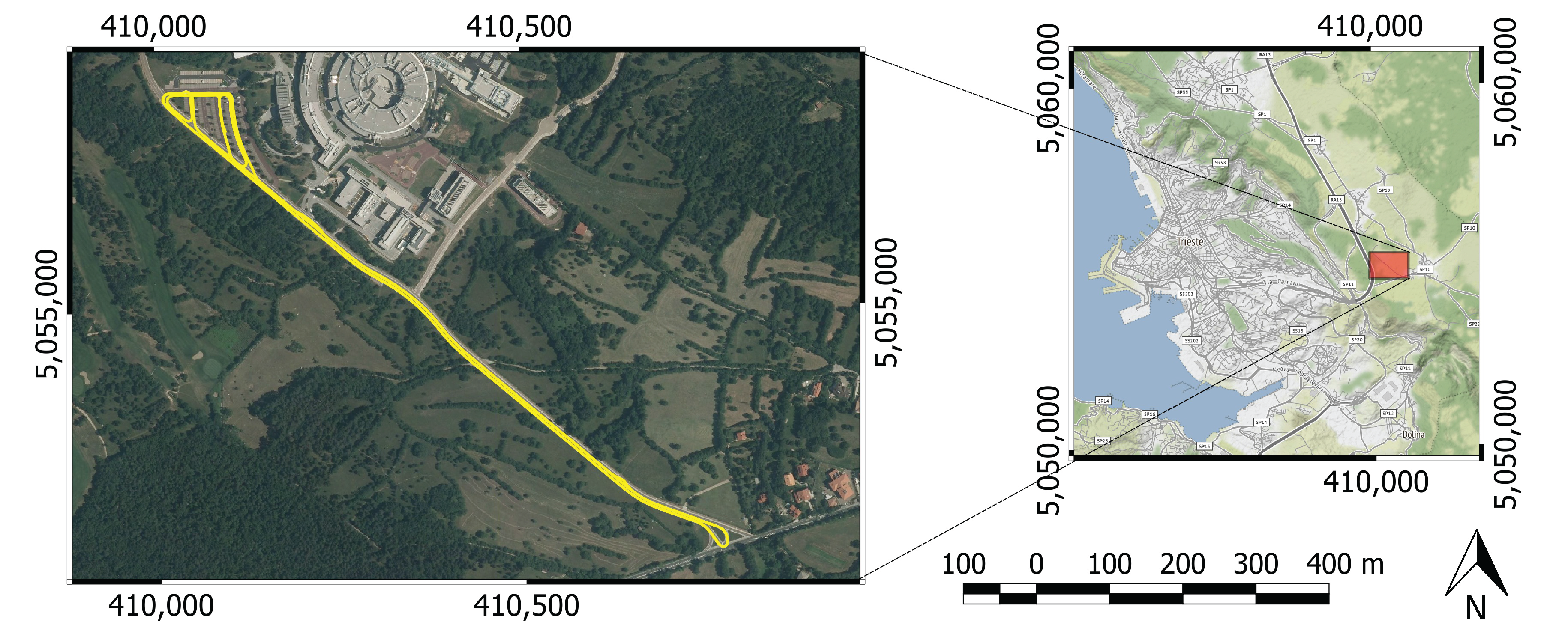
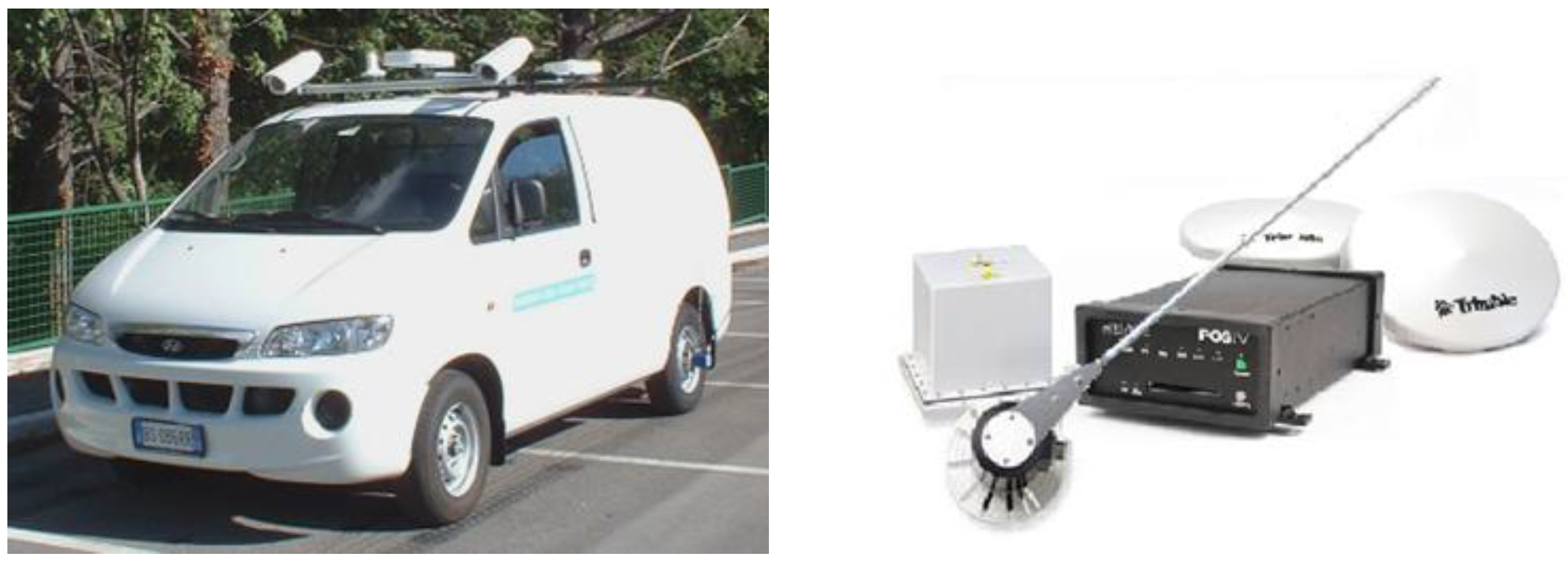
2.1. Experiment Location and MMS POS/LV Description and Configuration

The kinematic tests were carried out in Basovizza, a district on the outskirts of the Municipality of Trieste, Italy. The researchers drove the MMS vehicle at constant speed along the internal paved roads of the Sincrotrone Elettra Research Center Park. This particular site was chosen in order to maximize satellite visibility and signal-to-noise ratio, as it is located on the Karst plateau, at an average altitude of 375 m above mean sea level, with a clear view on all sides. The only relevant visibility obstacle is Mount Cocusso (674 m), located at 3.5 km in the NE direction (Figure 1).
For the absolute positioning, the Mobile Mapping System uses the Applanix Corporation POS/LV System, a fully integrated, position and orientation system, with GNSS positioning integrated by inertial technology to generate stable, reliable, and repeatable positioning solutions for land-based vehicle applications (Figure 2). Designed to operate under the most difficult GNSS conditions in urban and suburban environments, it enables accurate positioning for road geometry, pavement inspection, GIS database and asset management, road surveying, and vehicle dynamics [42]. The integrated GNSS/INS (Global Navigation Satellite System/Inertial System) is able to provide, instant by instant, the position and attitude of the vehicle. Besides the two geodetic GNSS receivers and the Inertial System, there is also an odometer mounted on the rear-left wheel of the vehicle, measuring the distance traveled. The inertial system integrates GPS in case of no satellite signal due to obstacles such as bridges, trees, buildings, to give positioning accuracies comparable to the ones obtainable through differential techniques. A Kalman filter, which allows to gain the best solution at any time, performs the integration of each sensor data. GNSS data has a 1 Hz acquisition rate, while the odometer and the inertial system send data to the System CPU at a rate of 200 Hz.
In the present research, all positioning data were referred to the Leica GS14 [43] receiver antenna phase center. This was done to directly compare, epoch by epoch, the positions computed using GS14 data with the MMS reference trajectory.
The PCS (POS Computer System) is the central element of the Applanix system: it acquires and processes data coming from the different sensors, giving the positioning and attitude parameters of the vehicle in real-time, and stores them for subsequent post-processing. The integrated inertial system is a Litton LN-200 fiber optic gyro IMU with three accelerometers and three fiber optic laser gyros. A DMI (Distance Measuring Indicator) is mounted on the rear-left wheel of the vehicle and contains an optical sensor generating 1024 pulses per revolution; its function is to estimate the run distance and, above all, to determine when the vehicle has come to a halt (ZUPD—Zero velocity UPDate). Two geodetic GPS receivers send the data to the PCS for positioning and direction determination, the latter utilizing the GAMS (GPS Azimuth Measurement Subsystem) software module.

2.2. Survey Experimental Design

The data for this experiment were acquired on the afternoon of July 25, 2017. Considering the reduced operation of the Galileo system, finding a place that could guarantee adequate visibility for a kinematic survey was not a trivial task. The location and the acquisition time were chosen to guarantee constant visibility of at least four Galileo satellites with a cut-off of 10° and six Galileo satellites for the major part of the survey. A peak of 11 GPS and 9 GLONASS satellites were respectively available during the survey (Figure 3).
Figure 3 shows the number of satellites and the geometric dilution of precision (GDOP—calculated by using the RTKPLOT tool) for the whole surveying session and clearly depicts the difference between the statuses of operability of the three positioning systems. The spikes in the GDOP plot are generally due to cycle slips or to a temporary loss of tracking of one or more satellites. From this point of view, the GPS constellation features the best configuration. It is worth mentioning that Galileo satellites occupied only the southern part of the Skyplot.
The full acquisition, made with both the GS14 receiver and the MMS, took almost one hour at a sampling rate of 1 Hz. Because of firmware restrictions, the GS14 was able to acquire only the E1 signal from the Galileo constellation. For this reason, the analysis was always referred to the E1, L1, and G1 signals acquired, respectively, from the Galileo, the GPS, and the GLONASS constellations. From the whole set of acquired epochs, only 1376 were used to perform the inter-constellations comparisons. This epoch selection was carried out accurately thanks to the MMS’ odometer with which only the kinematic part of the survey was considered. The vehicle, equipped with both the MMS and the GS14, completed the whole route four times. Before the beginning of each round on the path, a static session of few epochs was executed only to initialize the fixing of the phase ambiguities for the reference trajectory before the beginning of the next trip. This was necessary also in order to fulfill the aim of testing all the possible satellite acquisition conditions during the survey (further details can be found in the next section). The data from the Leica Smartnet ItalPoS network [44,45] were used to compute the differential post-processed trajectory related to the GS14 receiver.

2.3. Data Processing and Comparison Method

The data process chain, implemented to perform the preliminary comparisons, can be summarized in three macro-phases:
  • GS14 differential single constellations trajectory computation for all the possible combinations of four, five, and six satellites;
  • Reference trajectory computation from MMS data;
  • Solutions filtering and comparisons.
As stated in the Introduction section of this paper, all the comparisons were performed under the hypothesis that the MMS solution was more precise than the single differenced constellation solutions. Each single constellation differential solution was achieved by means of the Free and Open-Source Software (FOSS) RTKLIB [46]. RTKLIB was chosen for its easily configurable CUI (command user interface [41]) by means of the python subprocess module [47]. Apart from the MMS output result computation, performed with the MMS-associated proprietary software, all the other computations, including the ones with RTKLIB, were launched or executed by using the Python 2.7 programming language and by exploiting the parallel computing Python multiprocessing package [48], whose time-saving capability has already been reported in the scientific literature [49].

2.3.1. Trajectories Computations from GS14 Data

The aim of the trajectories computations was to produce differential solutions for the whole set of GS14 acquired data and to perform the subsequent comparisons. Each computation was executed by using the RNX2RTKP CUI tool of RTKLIB [41] and permanent station data (used to produce a post-processed kinematic solution). For this purpose, a separate RNX2RTKP configuration file was created for each calculated trajectory (see Table 1) by means of a Python function created ad hoc.
To perform a fair comparison among the computed trajectories of the single constellations, a reduced operativeness was simulated considering the maximum available number of Galileo satellites (six) for the performed kinematic survey. All the possible results obtained for all the combinations of four, five, and six satellites of the individual GPS and GLONASS constellations were respectively compared with all the possible results obtained for all the combinations of four and five satellites (and with the unique combination of six satellites) of the individual Galileo constellation. The number of potentially produced trajectories can be calculated as the number of satellite combinations with k dimension, without repetitions, taken from the whole set of available satellites. This number is given by the binomial coefficient (Equation (1)):
( n k ) = n ! k ! ( n k ) !
where n is the number of available satellites (11, 9, and 6, respectively, for GPS, GLONASS, and Galileo constellations), and k is the number of the considered satellites for each produced combination (four, five, and six).
RNX2RTKP has a wide range of parameters (almost 100) that can be modified within the configuration file to achieve different solutions. In our case, for each tested satellite combination and for each individual constellation, we opted for the following RNX2RTKP main configuration parameters: (1)the kinematic solution for the whole survey (to create a trajectory of points); L1 frequency (single-frequency analysis for the E1, L1, and G1 signals); broadcasted ionospheric model and Saastamoinen tropospheric model; forward Kalman filtering. For each combination, three different cut-off angles (10°, 15°, and 20°) and three different integer ambiguity resolution strategies were tested (Continuous, Instantaneous, and Fix and Hold). Moreover, the configuration file allows the user to select one or more constellation and to exclude user-defined satellites for the computations. This feature was exploited to simulate the reduced operativeness. All the other configuration parameters were not changed (further details on the algorithms implemented in RTKLIB can be found in [41]). In this way, for each selected satellite combination, nine different solutions were computed. As shown in Section 2.3.3 (Data filtering and comparisons), among these nine solutions for each combination, potentially only one (the best, according to Equation (6) and the previous applied filters) would represent the selected combination. Table 1 reports the number of solutions (and thus the trajectories potentially computed) for the combinations of four, five, and six satellites for each constellation.
The most important RNX2RTKP solution data are: latitude, longitude, and ellipsoidal height, a quality flag (in this case 1 for a fixed solution and 2 for a float solution), the number of used satellites, all the variance and covariances related to the 3D solution uncertainties. All the geographic coordinates were projected to the RDN ETRS89-ETRF2000 reference system using the Python PyProj package [50]. The PyProj package is the Python interface to PROJ.4 library and, for the purposes of this study, can be considered accurate, since it is also involved in the “VERTO” online coordinate converter [51], courtesy of the IGM (Italian Geographic Military section). Coordinate projections were performed, since we found it more convenient to assess the comparisons by using projected coordinates.
It is worth mentioning that, as a consequence of the simulated reduced operativeness for the three constellations, not all the RTKLIB solutions, composed by only a few computed epochs, were able to produce a significant output trajectory. For this reason, all the RTKLIB solutions characterized by a percentage of fixed epochs less than 1% of the whole survey (almost 4000 epochs, sampling rate 1 Hz) were excluded from the subsequent computation. Table 2 shows the number of remaining solutions after this first filtering process. Lastly, for the GS14 RNX2RTKP trajectory computation, the whole set of acquired epochs was used to compute the trajectories point by point. As mentioned in Section 2.2 (Survey experimental design), the static epochs recorded were used only to increase the probability to achieve an RNX2RTKP fixed solution before the beginning of the kinematic path. According to the purpose of this study, for the subsequent comparisons (see Section 2.3.3), only the RNX2RTKP solution data related to the kinematic epochs of the survey were considered.

2.3.2. Reference Trajectory: MMS Output

The 3D post-processed MMS output trajectory was used as a reference for the subsequent data filtering and comparisons. This assumption was the main working hypothesis of the experiment and is based on the following description.
The POS/LV system provides in output more than fifty data fields. Among the computed data, there are: positioning parameters (latitude, longitude, and ellipsoidal height), run distance, vehicle attitude (roll, pitch, and yaw angles), speed with respect to North, East, and z axes, accelerations, angular speeds, measurements rms.
The POS/LV system is built to integrate the data acquired from the different sensors, monitoring their health, isolating the sensors showing degraded performances, and re-configuring, conveniently weighting data inputs so as to give, in any case, the best positioning and attitude values. Sensor errors are estimated on a continuous basis using a Kalman filtering technique.
The system was calibrated thanks to the lever arms computed to give the positioning data of each point of the vehicle. Thanks to this feature, the MMS reference trajectory was referred to GS14 antenna phase center position. In order to compute the lever arms and the reciprocal positions of the GPS antennas, a reflector-less total station was used.
The reference trajectory was computed by post-processing the integrated GPS/INS data surveyed by the MMS. To this aim, the Position and Orientation System Post-Processing Package (POSPac™) Mobile Mapping Suite (MMS™) was used [52]. POSPac MMS with IN-Fusion™ technology (which provides a deep level of sensor integration and error modeling) allows multiple processing modes to handle different combinations of rover and reference GNSS data. IN-Fusion uses a centralized filter approach to combine the GNSS receiver’s pseudo-range and phase observables with the IMU data. As a result, the Applanix IN-Fusion technology has continual access to all GNSS, supplying information even if the GNSS receiver is tracking fewer than four satellites.
On the basis of the aforementioned MMS features, the formulated working hypothesis can be accepted, considering that: (I) the GS14 trajectories were computed to simulate a reduced operativeness for the GPS and the GLONASS systems (without exploiting the whole number of available satellites); (II) the MMS solution was computed using all the available GPS satellites with certified algorithms able to fuse GNSS L1 + L2 measurements with inertial data. Thus, a more accurate post-processed kinematic solution was ensured with respect to the GS14 one.

2.3.3. Data Filtering and Comparisons

The kinematic trajectories comparisons were executed calculating epoch by epoch the differences between the GS14 positions and the reference trajectory. Since special attention was given to the novel Galileo constellation, its results, for the combinations of four, five, and six satellites, were also compared with the analogous results of GPS and GLONASS systems and statistically assessed.
From the POSPac™ solution (Figure 1—reference trajectory), and by using the ZUPD feature, the kinematic epochs were identified. These epochs, for the purposes of this study and according to Section 2.2 and Section 2.3.1, were used to extract only the kinematic part of the solutions both for the MMS system and for all the previously computed trajectories (see Section 2.3.1 and Table 2).
For each epoch of each kinematic RNX2RTKP solution, the deviations of the GS14 trajectories and the reference trajectory were calculated in terms of Δ Ei , Δ Ni , Δ Hi , and Δ Di (Equations (2)–(5)—the “i” subscript indicates that these quantities are scalar and referred to the i-th epoch, otherwise they have to be considered as vectors). E, N, and H are the East and North coordinates and the ellipsoidal height, respectively.
Δ E , i = E MMS , i E RTKLIB , i ;
Δ N , i = N MMS , i N RTKLIB , i ;
Δ H , i = | H MMS , i H RTKLIB , i | ;
Δ D , i = ( Δ E , i ) 2 + ( Δ N , i ) 2 .
Δ D , i and the Δ H , i were used to compare the planimetric and altimetric performances of the Galileo system with regard to GPS and GLONASS. In particular, all the computed GS14 kinematic trajectories featuring at least one | Δ D , i | > 5   m were excluded to select only the potentially best combinations. Indeed, in this phase, a planimetric deviation of 5 m from the reference trajectory was considered an acceptable threshold to include float comparisons in the next computations. According to Section 2.3.1, it is worth noting that this constraint caused a further exclusion of some tested satellites combinations for the three constellations.
The last filtering process was introduced to select the best solution, among the nine potential solutions produced for each selected satellite combination (see Section 2.3.1), by considering the deviations Δ D and the Δ H and the quantity of produced fixed solutions ( % Q 1 ) for each considered GS14 derived trajectory. In this case, Δ D and Δ H were considered as the vectors constituted by the Δ D , i and the Δ H , i computed for each epoch. Lastly, the percentage of fixed solutions % Q 1 was always calculated considering the number of kinematic epochs (1376 see Section 2.2). This task was executed by implementing the following objective function (Equation (6)) specifically designed to handle the data produced starting from the kinematic survey:
f j , k , c ( Δ D , Δ H ,   % Q 1 ) = min { [ ( Δ D ¯ w Δ D ) + ( Δ H ¯ w Δ H ) w Δ D + w Δ H ] [ % Q 1 ] 1 }
f j , k , c is the value of the objective function computed for the k-th (with k potentially ranging from 1 to 9) solution, for the j-th considered satellite combination of four, five, or six satellites, and for the c-th considered constellation (Galileo, GPS, GLONASS); Δ D ¯ and Δ H ¯ are the average Δ D and Δ H values for the considered k, j, and c; w Δ D and w Δ D are the inverse of the variances of the Δ D and Δ H vectors for the considered k, j, and c. Lastly, if % Q 1 was equal to 0, then it was fixed at 0.07%, which was less than one fixed epoch over 1376 kinematic ones. Equation (6) can be considered as the product of a weighted mean of the planimetric and altimetric deviations multiplied by the inverse of the percentage of fixed solutions. It was designed to create a trade-off among solutions, considering the goodness of the deviations (thus the discrepancies from the reference trajectory) and the quality of the solutions (fixed or float). In this way, if a computed GS14 trajectory was characterized by good deviations towards the reference trajectory (thus, small Δ D ¯ and Δ H ¯ ) but with a low percentage of fixed solutions, there were few probabilities that it would be chosen when compared to solutions with slightly different deviations but characterized by a higher fix percentage.
After the application of the objective function (Equation (6)), 48 vectors for each of the 1376 kinematic epochs, were created to perform the comparisons:
(a)
16 vectors for the 4, 5, and 6 satellites combinations;
(b)
Among the 16 vectors for the considered combination (e.g., of 4 satellites), 8 vectors were generated for Galileo and GPS comparisons, and 8 vectors were generated for Galileo and GLONASS comparisons;
(c)
Considering, for example, Galileo and GPS comparisons (the same is valid for Galileo and GLONASS comparisons), the 8 vectors were produced by 4 couples of vectors finally used for the comparisons;
(d)
The 4 couples were built using, for each considered epoch (t), all the values found for the considered epoch t for planimetric and altimetric deviations, separated for fixed and float solutions. That is (e.g., for Galileo and GPS comparisons):
  • (I): two vectors Δ D , t referred to the t-th epoch in case of fixed solutions (one for Galileo and one for GPS system);
  • (II): two vectors Δ D , t referred to the t-th epoch in case of float solutions (one for Galileo and one for GPS system);
  • (III): two vectors Δ H , t referred to the t-th epoch in case of fixed solutions (one for Galileo and one for GPS system);
  • (IV): two vectors Δ H , t referred to the t-th epoch in case of float solutions (one for Galileo and one for GPS system);
(e)
Particularly, for each considered couple of vectors (e.g., couple I) related to a specific epoch t, the mean values for the Galileo analyzed parameter and for the same GPS (or GLONASS) parameter were computed and compared;
(f)
If the length of the considered GPS (or GLONASS) vector, referred to the t-th epoch, was greater than 15, a one-sample t-test [53] was executed to establish if the GPS (or Galileo and GLONASS) average parameter values were statistically different from the same Galileo parameters.

3. Results

3.1. MMS Reference Trajectory and RKTLIB Results

The differential solutions computed with the RNX2RTKP CUI tool were achieved by using a local reference station different (see acknowledgment) from the one used for the reference trajectory (i.e., the MMS one). The reason for this was that the reference station data (free of charge) used for the MMS solution had not yet included the Galileo acquisitions. The mean distance between the reference GNSS station and the vehicle, mounting both the MMS POS/LV system and the GS14 receiver, was less than 5 km.
Table 3 depicts the results of the application of Equation (6) used to select one solution (the “best” according to f j , k , c ) for each tested combination. It is worth mentioning that, for the application of Equation (6), it was necessary to select, among the available nine different solutions produced for each satellite combination (see Section 2.3.1), only the one that minimized the objective function. Hence, the final comparisons of the three constellations were made only among the best solutions and not among all those produced. The number of RTKLIB remaining trajectories (“n. of combinations” column), the percentage of occurrence of the cut-off angles, and the percentage of occurrence of the ambiguity fix with the implemented methods achieved through the application of Equation (6) (see Section 2.3.3), are shown in Table 3 for the available combinations. For example, the “best_gal_4” row reports the previous data for the remaining 13 combinations (and thus trajectories), according to Equation (6), obtained with different sets of four Galileo satellites.
Comparing the number of combinations shown in Table 3 with the ones featured in Table 1, an expected trend is evident, in which the percentage of selected combinations increases with the number of the considered satellites. Moreover, a clear difference between the Galileo, the GLONASS, and the GPS systems emerges from the cut-off angles associated to the best solution for each considered combination. This could be related to the increasing number of Galileo cycle slips (or loss of satellite tracking) occurred at lower elevation angles, whereas the opposite occurred for the other two constellations because of the availability of many combinations with satellites characterized by high elevation angles. Moreover, the experimental results for the GPS and GLONASS constellations showed a high occurrence of good solutions achieved through the “fix and hold” method. This experimental evidence showed, in this case, a quite stable behavior of the RTKLIB RNX2RTKP CUI tool for the GPS and GLONASS constellations. The same did not occur for the Galileo constellation and there could be several reasons to justify these differences. First of all, because of the reduced operativeness status of the Galileo constellation, a very small number of combinations could be tested (see Table 1, Table 2 and Table 3). As such, because of the higher number of combinations, only the first row of Table 3 (“best_gal_4”) should be considered as the most reliable Galileo information. Another reason could be related to a better overall performance of the Galileo constellation. Indeed, the second row in Table 3 (best_gal_5) indicates a prevalence of the “Instantaneous” ambiguity fixing method, the most conservative among the ones proposed by RTKLIB (appendix E.7 [41]).
The whole path length MMS solution was 4803 m. Since the distance between the survey area and the nearest reference station (named “Trieste” and belonging to the “Antonio Marussi” network, managed by “Regione Friuli Venezia Giulia” [54]) was in the range of 5–6 km, a network solution was not required. In particular, the “IN-Fusion Single-Base Station Processing” mode was chosen, processing both L1 and L2 frequencies and reaching centimetric rms both in planimetric and altimetric positioning.

3.2. Comparisons Results

A total of 24 couples of vectors were compared, when possible, for each t-th epoch (48 vectors produced for each epoch). The comparisons were executed in terms of Δ D and Δ H , thus in terms of discrepancy with respect to the MMS reference trajectory. The evaluations were performed for the four couple of vectors mentioned in point (d) of Section 2.3.3 for each t-th epoch. Particularly, considering the comparison strategy described in Section 2.3.3, for a considered epoch (t) and on equal footage, the comparisons were executed only if it was possible to calculate at least one value for the considered parameter ( Δ D or Δ H ), for the Galileo t-th epoch and at least one value for the GPS (or GLONASS) t-th epoch. For this reason, the second column in Table 3 (n. of combinations) also provides the potential maximum lengths of the compared vectors: e.g., considering the comparison between the Δ D computed with fixed solutions for all the combinations of four satellites, the maximum length for a vector associated to a t-th epoch was 13 for Galileo and 77 for GPS. Moreover, considering the number of solutions for one selected epoch, the presence of both fixed and float solutions was highly probable and, again, the second column in Table 3 gives the potential maximum lengths of the compared vectors.
The tests involved a huge amount of generated data produced in order to consider and compare the average behavior of all possible operative conditions in a real case study, thus simulating all the real working conditions with a virtual reduced operativeness. The results for the 24 couples of comparisons are summarized in Table 4, and, in the Appendix section, only four images (enclosed in Figure A1) related to the grey rows in Table 4 are provided. For clarity and to avoid a bulky manuscript, the remaining 20 images (related to the remaining 20 rows) are provided as Supplementary Material (Figures S1–S20).
Table 4 shows, for each comparison, the global results of the comparisons performed epoch by epoch and the global results of the statistical tests:
  • Each entry in the “comparison” column in Table 4 shows the object of the comparison: “ Δ D , 1 gal_vs_gps_4” and “ Δ D , 2 gal_vs_gps_4” are, respectively, the comparisons between the Δ D parameter for fixed ( Δ D , 1 ) and float ( Δ D , 2 ) solutions for the combination of four satellites of the Galileo and GPS systems;
  • The average values comparison (Avg. values comp.) columns report:
    the number of epochs for which it was possible to execute the simple comparisons between the average values of the two vectors;
    the number of times (gal score), expressed in percentage, in which the considered Galileo average planimetric or altimetric deviations performed better (thus was closer to the reference MMS trajectory for the t-th epoch).
  • The columns related to the t-test summary report:
    the number of epochs in which it was possible to execute the one-sample t-test (point f) Section 2.3.3);
    the average p-value, introduced to provide a global vision of statistical significance of the tested differences;
    the number of epochs, expressed in percentage, in which the p-value was less than 0.5.
  • Lastly, the Appendix/Supp. Material columns provide the references to the Appendix/Support Material figures. The reader should bear in mind that the presented figures and results derive from trajectories computed in post-processing with different accuracies (see Section 2.3.2).
Table 4 shows, for the performed kinematic test, an evidence of the better planimetric performance of the Galileo system (the first 12 rows of Table 4). This experimental evidence becomes even stronger with the increasing number of satellites, regardless of the considered constellation. In the Galileo-GPS and Galileo-GLONASS comparisons, the GPS performed slightly better than the GLONASS system. Indeed, the “gal score” related to the GLONASS comparisons was always higher than the one associated to the GPS comparisons. Another important output was the number of fixed solutions produced by the Galileo combinations. In fact, the reduced number of Galileo available satellites allowed a very small number of satellite combinations. Despite this, it was possible to produce 1287 comparisons for the “ Δ D , 1 gal_vs_gps_5” group. This cannot be considered a causality since Table 3 also shows that the Galileo combinations with five satellites were the ones in which there was a prevalence of the “Instantaneous” ambiguity fixing method (the most restrictive one). With regard to the number of epochs involved in the computations of float comparisons, Table 4 shows a very high decreasing rate when the combinations with six satellites were involved. This is true both for of Δ D 2 and Δ H 2 and is a direct consequence of the increasing number of satellites associated with a higher rate of fixed ambiguities.
The statistical assessment data of the Δ D 1 and Δ D 2 results in Table 4 provide a summary of the outcomes. In this case, the aim was to test if the found differences were statistically significant and which percentage of these differences could be considered at the 5% significance level. The lower the p-value, the stronger the statistical significance of the differences will be. No statistical tests were performed over the “gal_vs_glo_4” groups, since the imposed conditions to perform the tests were not satisfied (see point f) Section 2.3.3). As expected, because of the higher number of available combinations, more tests were performed with the GPS system. With regard to Δ D 1 and Δ D 2 comparisons, Table 4 depicts a common scenario both for the fixed and the float solutions. The found differences became more significant when the number of satellites rose. They reached the maximum statistical significance in the “ Δ D , 1 gal_vs_gps_6” comparison. An empirical evidence of the better Galileo performance characterized by planimetric solutions closer to the MMS trajectory, when comparing the previous columns with these data, is evident for this real case study. Also Figure A1a (see Appendix) reveals that, when the GPS system performed better, the found differences were not significant (the green point depicts quite elevated p-values). With regards to the “ Δ D , 1 gal_vs_glo_6” group, despite the superiority of the Galileo system (Figure A1b), the lower degree of statistical significance (if compared to the “ Δ D , 1 gal_vs_gps_6”) could also be due to the lower number of GLONASS combinations.
From the altimetric point of view (able 4: rows 13 to 24), the proposed scenario shows a better performance of GPS and GLONASS systems. However, the “gal score”, in this case, empirically indicates that this evidence is not as strong as in the case of the planimetric analysis. Table 4 also demonstrates a positive trend for the “gal score” coupled with the increasing number of satellites. As far as the statistical assessment of the altimetric comparison is concerned, a lower rate of statistical significance depicted both by average p-value and by the number of tested epochs with a p-value < 0.05 coould be seen. This is clearly shown in Figure A1c,d (see Appendix), in which the lower degree of statistical significance is particularly marked for the “ Δ H , 1 gal_vs_glo_6” (Figure A1d—the green points related to the p-values). This empirical evidence, encountered especially in the altimetric comparisons, can be explained by the lower altimetric accuracy of the analyzed solutions. Therefore, The lower Galileo altimetric accuracy may be related to a nonoptimal vertical configuration of the satellites available for the kinematic surveys.
Lastly, the figures listed in Table 4 and provided as Supplementary Material feature a detailed visual output of the performed tests. The description useful for their interpretation can be found in the Appendix section.

4. Discussion

In this study, the comparison between Galileo, GPS, and GLONASS satellite positioning systems was proposed for a kinematic survey. The GNSS data were acquired with a Leica™ GS14 receiver and compared with the output obtained by a Mobile Mapping System (MMS), implementing integrated high-performance GPS/INS measurements. In particular, as far as the authors know, this is the first work that uses a precise MMS trajectory for the assessment of the kinematic performances of the Galileo system.
All the differential solutions were produced with the open-source set of libraries RTKLIB. Particularly, the RTKLIB CUI was used to simulate a reduced operational status for the GPS and GLONASS systems. Specifically, thanks to the RTKLIB CUI capabilities, it was possible, by using the Python programming language, to contemporarily execute many solutions. Indeed, the aim was to produce and compare, in sets of four, five, and six satellites, all the possible and real acquisition scenarios occurring during the survey.
In the authors' opinion, this experiment can be considered as a preliminary stress test for the Galileo system to verify if it has the potentiality to overpass the performances of the previous systems. Despite the effort to produce a fair comparison, the limited amount of Galileo satellites and their geometrical configuration (Figure 3) put the Galileo system in a disadvantaged position with respect to the other two analyzed systems. This remains true even if the whole survey was planned to maximize the number of available Galileo satellites. Indeed, the displayed performance, especially from a planimetric point of view, cannot be justified only by the fact that the whole survey was organized to maximize the probability of Galileo acquisitions. This can also be understood by considering the filtering strategy adopted before the applications of Equation (6), and the results of the application of Equation (6), used to select the solutions that were compared. A first important result was represented by the presence of Galileo combinations able to pass the filtering process. This was necessary to build the next comparisons by applying the objective function. In fact, the aim of Equation (6) was to select only the best solutions (low deviations with respect to the MMS solution) and, among these, to choose the ones characterized by a high fix rate. Equation (6) was applied, without any other constraint, to the three analyzed constellations. However, the difference between Galileo and the other tested systems relied on the different number of possible combinations that, in some cases, was of two orders of magnitude (Table 3).
For these reasons, the fact that the planimetric results are very encouraging should be considered, as stated by other researchers (e.g., [3,4,5,10]), also in relation to the lower level of Galileo signal noise. From an altimetric point of view, the results were different. However, because of the lower level of statistical significance (not as clear as in the planimetric case) and the higher performance correlated to the increasing number of satellites shown in Table 4, there is the need to analyze more data to properly assess the altimetric performances. In the authors’ opinion, the very small number of available combinations for the Galileo system and the non-uniform distribution in the visible satellite elevations were responsible for the lower altimetric performances.
Another result of this work is related to the experimental use of the software RTKLIB. The results performed for many combinations show a high occurrence of good solutions achieved with the “fix and hold” method for the GPS and GLONASS constellations. In case of post-processed analysis, this result can be instrumentally time-saving for those interested in using the RTKLIB set of tools. The same cannot be said for the Galileo constellation because of the lower amount of available satellites.

5. Conclusions

In this study, a big computational effort was produced to analyze 1 Hz multi-constellation kinematic data acquired during a one-hour field survey, planned to maximize Galileo satellites availability. The acquired data included a contemporary acquisition through an MMS equipped with a POS/LV produced by the Applanix corporation. The MMS acquisition was used as a reference trajectory, and the robustness of its solution was the most important hypothesis for the results shown in this study. This hypothesis can be considered always valid for research since it was found by coupling the GNSS technology with precise inertial instruments. Moreover, the MMS solution was calculated considering a higher amount of GNSS satellites when compared with the number of satellites used to perform the tests (four, five, and six). Lastly, only the L1, G1, and E1 frequencies were used in this experiment.
In order to present a real kinematic comparison between Galileo, GPS, and GLONASS satellite positioning systems, a reduced operational status was simulated for GPS and GLONASS. Moreover, it was possible to implement post-processed differential solutions with the Open-Source Software RTKLIB, thanks to the GNSS acquisitions of reference stations close to the surveyed areas.
The performed comparisons, whenever possible, were analyzed also by means of a statistical test. The outputs showed a clear and statistically significant planimetric performance of the Galileo positioning system, whereas the same result was not obtained from an altimetric point of view. However, in the authors’ opinion, this was especially due to the very small number of Galileo satellites and to their geometrical configurations.
Although these results were obtained with several computations, especially for the Galileo altimetric performance, they need to be reinforced by further experimental evidence. For this reason, they should be considered as preliminary results achieved by using a reference trajectory. Moreover, it is possible to conclude that the novel system is very promising also when used alone; in a disadvantaged comparison, it was able to produce better planimetric accuracy than the GPS and GLONASS positioning systems in a kinematic survey.
Future development of this work can include the kinematic inter-constellation comparison, the evaluation of the robustness of velocity and acceleration estimation with the Galileo constellation, and attitude estimations.

Supplementary Materials

The following are available online at https://www.mdpi.com/2220-9964/7/3/122/s1. For a description of the following figures, please see the Appendix section. Figure S1: Δ D , 1 gal_vs_gps_4, Figure S2: Δ D , 1 gal_vs_glo_4, Figure S3: Δ D , 1 gal_vs_gps_5, Figure S4: Δ D , 1 gal_vs_glo_5, Figure S5: Δ D , 2 gal_vs_gps_4, Figure S6: Δ D , 2 gal_vs_glo_4, Figure S7: Δ D , 2 gal_vs_gps_5, Figure S8: Δ D , 2 gal_vs_glo_5, Figure S9: Δ D , 2 gal_vs_gps_6, Figure S10: Δ D , 2 gal_vs_glo_6, Figure S11: Δ H , 1 gal_vs_gps_4, Figure S12: Δ H , 1 gal_vs_glo_4, Figure S13: Δ H , 1 gal_vs_gps_5, Figure S14: Δ H , 1 gal_vs_glo_5, Figure S15: Δ H , 2 gal_vs_gps_4, Figure S16: Δ H , 2 gal_vs_glo_4, Figure S17: Δ H , 2 gal_vs_gps_5, Figure S18: Δ H , 2 gal_vs_glo_5, Figure S19: Δ H , 2 gal_vs_gps_6, Figure S20: Δ H , 2 gal_vs_glo_6.

Acknowledgments

The authors thank Leica for their technical support and for giving access to SmarNet ItalPos Galileo data used for the processing and analyses presented in this paper.

Author Contributions

All the authors equally contributed to the experimental design (including the field survey) and manuscript revision of this work. Moreover, Antonio Novelli made the parallel computations using the Python programming language and RTKLIB.

Conflicts of Interest

The authors declare no conflict of interest.

Appendix A

This Appendix shows the Figure A1a–d mentioned in Table 4 and in Section 3.2. The remaining set of figures, listed in Table 4, are provided as supplementary material (see Supplementary Material section). The aim of these figures is to provide a detailed visual representation of the performed comparisons, each of which is organized as follows:
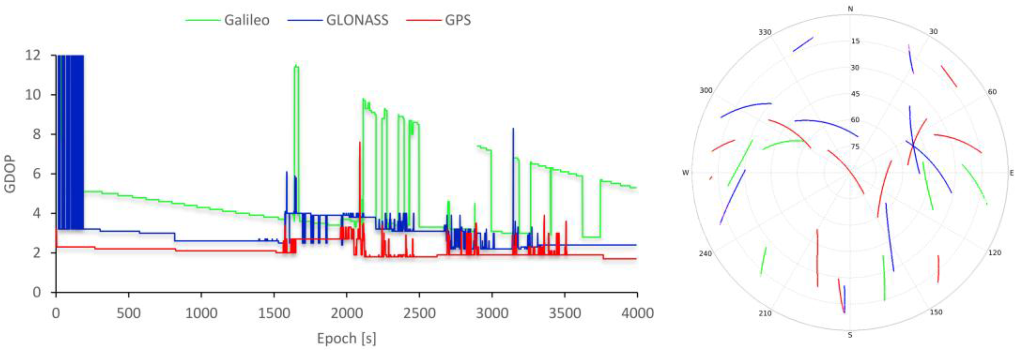
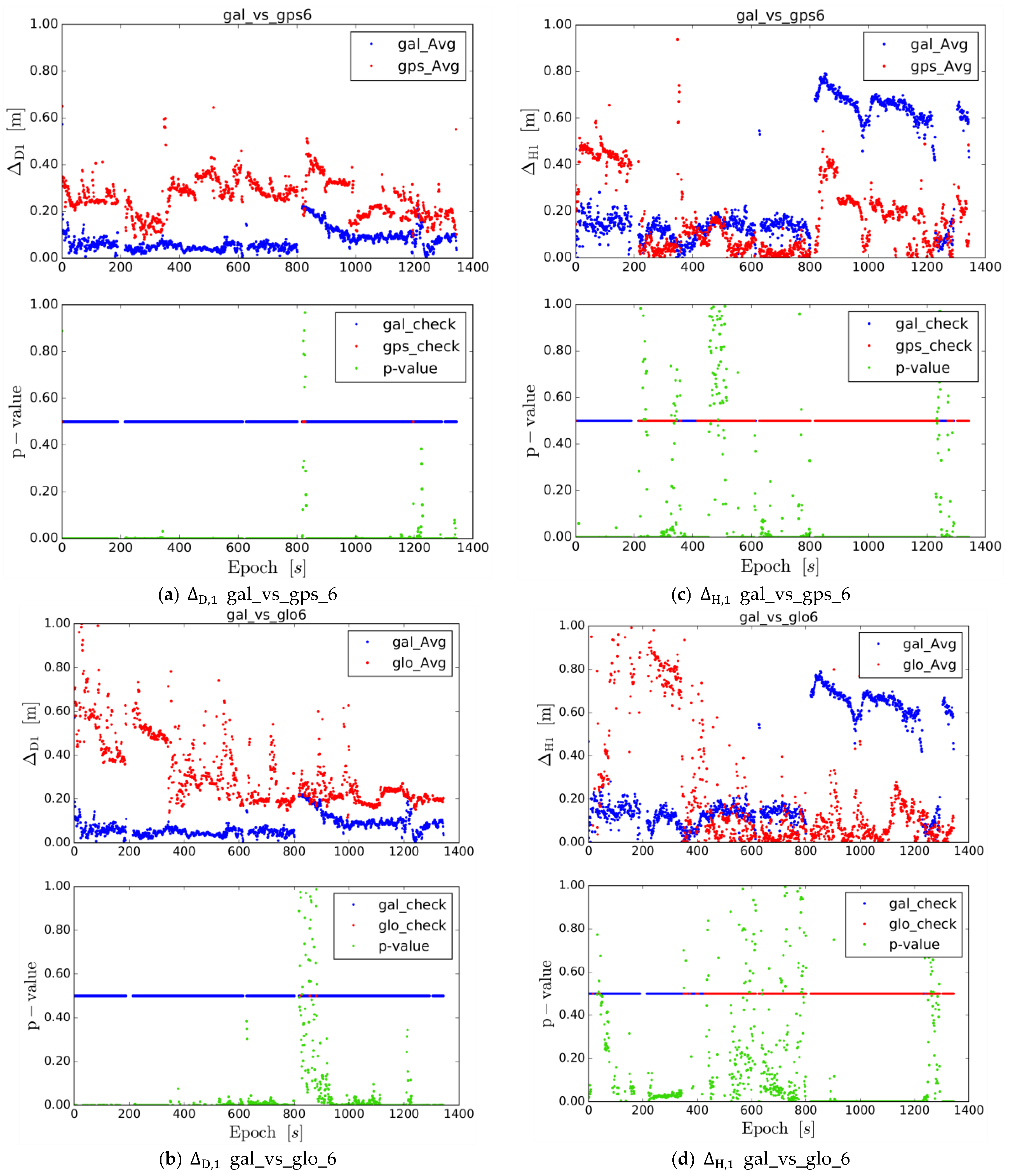
  • The Galileo data are provided in blue, the GPS and GLONASS data in red, the p-values in green;
  • The average Δ values of the comparisons (“gal_Avg” for Galileo, gps_Avg for GPS, and glo_Avg for GLONASS) are provided in the upper subplot, whereas the statistical significance (p-value) of the differences is shown in the lower subplot;
  • The lower subplot reports also additional information with a horizontal line placed at an ordinate of 0.5. This line is blue (gal_check) when the Galileo system performed better and is red (gps_check or glo_check) when the GPS of the GLONASS Systems performed better;
  • The high degree of scattering of the p-value indicates a low statistical significance for the related epochs;
  • The plots show the comparison for fixed solutions if the subscript of the parameter on the ordinate of the upper subplot is 1 (e.g., Δ D , 1 and Δ H , 1 );
  • The plots show the comparison for float solutions if the subscript of the parameter on the ordinate of the upper subplot is 2 (e.g., Δ D , 2 and Δ H , 2 ).
Figure A1. Visual output of the performed test: (a) Δ D , 1 gal_vs_gps_6, for Galileo and GPS comparison considering all the fixed solutions (1 in the subscript) for the Δ D parameter with six considered satellites; (b) Δ D , 1 gal_vs_glo_6, for Galileo and GLONASS comparison considering all the fixed solutions (1 in the subscript) for the Δ D parameter with six considered satellites; (c) Δ H , 1 gal_vs_gps_6, for Galileo and GPS comparison considering all the fixed solutions (1 in the subscript), for the Δ H parameter with six considered satellites; (d) Δ H , 1 gal_vs_glo_6, for Galileo and GPS comparison considering all the fixed solutions (1 in the subscript) for the Δ H parameter with six considered satellites.
Ijgi 07 00122 g0a1

References

  1. ESA: Galileo Fact Sheet. Available online: http://esamultimedia.esa.int/docs/galileo/GalileoFactsheet2017.pdf (accessed on 14 December 2017).
  2. Steigenberger, P.; Hugentobler, U.; Montenbruck, O. First demonstration of Galileo-only positioning. GPS World 2013, 24, 14–15. [Google Scholar]
  3. Simsky, A.; Mertens, D.; Sleewaegen, J.-M.; Hollreiser, M.; Crisci, M. Experimental results for the multipath performance of Galileo signals transmitted by GIOVE-A satellite. Int. J. Navig. Obs. 2008, 2008, 416380. [Google Scholar] [CrossRef]
  4. Simsky, A.; Mertens, D.; Sleewaegen, J.-M.; De Wilde, W.; Hollreiser, M.; Crisci, M. Multipath and tracking performance of Galileo ranging signals transmitted by GIOVE-B. In Proceedings of the 21st International Technical Meeting of the Satellite Division of the Institute of Navigation (ION GNSS), Savannah, GA, USA, 16–19 September 2008; pp. 1525–1536. [Google Scholar]
  5. Simsky, A.; Sleewaegen, J.-M.; Hollreiser, M.; Crisci, M. Performance assessment of Galileo ranging signals transmitted by GSTB-V2 satellites. In Proceedings of the ION GNSS, Fort Worth, TX, USA, 26–29 September 2006; pp. 1547–1559. [Google Scholar]
  6. Hellemans, A. A Simple Plumbing Problem Sent Galileo Satellites into Wrong Orbits. Available online: https://spectrum.ieee.org/tech-talk/aerospace/satellites/a-simple-plumbing-problem-sent-galileo-satellites-into-wrong-orbits (accessed on 14 December 2017).
  7. Langley, R.B. ESA Discusses Galileo Satellite Power Loss, Upcoming Launch. Available online: http://gpsworld.com/esa-discusses-galileo-satellite-power-loss-upcoming-launch/ (accessed on 14 December 2017).
  8. European Union. Galileo Open Service, Signal in Space Interface Control Document (OS SIS ICD); European Space Agency/European GNSS Supervisory Authority. Available online: https://www.gsc-europa.eu/system/files/galileo_documents/Galileo-OS-SIS-ICD.pdf (accessed on 14 December 2017).
  9. ESA. Galileo: A Constellation of Navigation Satellites. Available online: http://www.esa.int/Our_Activities/Navigation/Galileo/Galileo_a_constellation_of_navigation_satellites (accessed on 11 December 2017).
  10. Zaminpardaz, S.; Teunissen, P.J. Analysis of Galileo IOV+ FOC signals and E5 RTK performance. GPS Solut. 2017, 21, 1855–1870. [Google Scholar] [CrossRef]
  11. Steigenberger, P.; Montenbruck, O. Galileo status: Orbits, clocks, and positioning. GPS Solut. 2017, 21, 319–331. [Google Scholar] [CrossRef]
  12. Ochieng, W.Y.; Sauer, K.; Cross, P.A.; Sheridan, K.F.; Iliffe, J.; Lannelongue, S.; Ammour, N.; Petit, K. Potential performance levels of a combined Galileo/GPS navigation system. J. Navig. 2001, 54, 185–197. [Google Scholar] [CrossRef]
  13. O’Keefe, K.; Julien, O.; Cannon, M.E.; Lachapelle, G. Availability, accuracy, reliability, and carrier-phase ambiguity resolution with Galileo and GPS. Acta Astronaut. 2006, 58, 422–434. [Google Scholar] [CrossRef]
  14. Diessongo, T.H.; Schüler, T.; Junker, S. Precise position determination using a Galileo E5 single-frequency receiver. GPS Solut. 2014, 18, 73–83. [Google Scholar] [CrossRef]
  15. Odijk, D.; Teunissen, P.J.; Huisman, L. First results of mixed GPS+ GIOVE single-frequency RTK in Australia. J. Spat. Sci. 2012, 57, 3–18. [Google Scholar] [CrossRef]
  16. Cai, C.; Luo, X.; Liu, Z.; Xiao, Q. Galileo signal and positioning performance analysis based on four IOV satellites. J. Navig. 2014, 67, 810–824. [Google Scholar] [CrossRef]
  17. Gaglione, S.; Angrisano, A.; Castaldo, G.; Freda, P.; Gioia, C.; Innac, A.; Troisi, S.; Del Core, G. The first Galileo FOC satellites: From useless to essential. In Proceedings of the 2015 IEEE International Geoscience and Remote Sensing Symposium (IGARSS), Milan, Italy, 26–31 July 2015; pp. 3667–3670. [Google Scholar]
  18. Gioia, C.; Borio, D.; Angrisano, A.; Gaglione, S.; Fortuny-Guasch, J. A Galileo IOV assessment: Measurement and position domain. GPS Solut. 2015, 19, 187–199. [Google Scholar] [CrossRef] [Green Version]
  19. Tegedor, J.; Øvstedal, O.; Vigen, E. Precise orbit determination and point positioning using GPS, Glonass, Galileo and BeiDou. J. Geod. Sci. 2014, 4. [Google Scholar] [CrossRef]
  20. Lou, Y.; Zheng, F.; Gu, S.; Wang, C.; Guo, H.; Feng, Y. Multi-GNSS precise point positioning with raw single-frequency and dual-frequency measurement models. GPS Solut. 2016, 20, 849–862. [Google Scholar] [CrossRef]
  21. Liu, T.; Yuan, Y.; Zhang, B.; Wang, N.; Tan, B.; Chen, Y. Multi-GNSS precise point positioning (MGPPP) using raw observations. J. Geod. 2017, 91, 253–268. [Google Scholar] [CrossRef]
  22. Pan, L.; Zhang, X.; Liu, J.; Li, X.; Li, X. Performance evaluation of single-frequency precise point positioning with GPS, GLONASS, BeiDou and Galileo. J. Navig. 2017, 70, 465–482. [Google Scholar] [CrossRef]
  23. Afifi, A.; El-Rabbany, A. Single Frequency GPS/Galileo Precise Point Positioning Using Un-Differenced and between-Satellite Single Difference Measurements. GEOMATICA 2014, 68, 195–205. [Google Scholar] [CrossRef]
  24. Cai, C.; He, C.; Santerre, R.; Pan, L.; Cui, X.; Zhu, J. A comparative analysis of measurement noise and multipath for four constellations: GPS, BeiDou, GLONASS and Galileo. Surv. Rev. 2016, 48, 287–295. [Google Scholar] [CrossRef]
  25. Pan, L.; Cai, C.; Santerre, R.; Zhang, X. Performance evaluation of single-frequency point positioning with GPS, GLONASS, BeiDou and Galileo. Surv. Rev. 2017, 49, 197–205. [Google Scholar] [CrossRef]
  26. Guo, F.; Li, X.; Zhang, X.; Wang, J. Assessment of precise orbit and clock products for Galileo, BeiDou, and QZSS from IGS Multi-GNSS Experiment (MGEX). GPS Solut. 2017, 21, 279–290. [Google Scholar] [CrossRef]
  27. Odijk, D.; Teunissen, P.J.; Khodabandeh, A. Galileo IOV RTK positioning: Standalone and combined with GPS. Surv. Rev. 2014, 46, 267–277. [Google Scholar] [CrossRef]
  28. Odolinski, R.; Teunissen, P.J.; Odijk, D. Combined bds, galileo, qzss and gps single-frequency rtk. GPS Solut. 2015, 19, 151–163. [Google Scholar] [CrossRef]
  29. Li, X.; Ge, M.; Dai, X.; Ren, X.; Fritsche, M.; Wickert, J.; Schuh, H. Accuracy and reliability of multi-GNSS real-time precise positioning: GPS, GLONASS, BeiDou, and Galileo. J. Geod. 2015, 89, 607–635. [Google Scholar] [CrossRef]
  30. Nadarajah, N.; Teunissen, P.J.G. Instantaneous GPS/Galileo/QZSS/SBAS Attitude Determination: A Single-Frequency (L1/E1) Robustness Analysis under Constrained Environments. Navigation 2014, 61, 65–75. [Google Scholar] [CrossRef]
  31. Nadarajah, N.; Teunissen, P.J.; Raziq, N. Instantaneous GPS–Galileo attitude determination: Single-frequency performance in satellite-deprived environments. IEEE Trans. Veh. Technol. 2013, 62, 2963–2976. [Google Scholar] [CrossRef]
  32. Zajdel, R.; Sośnica, K.; Bury, G. A New Online Service for the Validation of Multi-GNSS Orbits Using SLR. Remote Sens. 2017, 9, 1049. [Google Scholar] [CrossRef]
  33. Carreno-Luengo, H.; Amèzaga, A.; Vidal, D.; Olivé, R.; Munoz, J.F.; Camps, A. First polarimetric GNSS-R measurements from a stratospheric flight over boreal forests. Remote Sens. 2015, 7, 13120–13138. [Google Scholar] [CrossRef] [Green Version]
  34. Cefalo, R.; Grandi, G.; Roberti, R.; Sluga, T. Extraction of Road Geometric Parameters from High Resolution Remote Sensing Images Validated by GNSS/INS Geodetic Techniques. In Proceedings of the Computational Science and Its Applications—ICCSA 2017, Trieste, Italy, 3–6 July 2017; Springer: Cham, Switzerland, 2017; Volume 10407, pp. 181–195, ISBN 978-3-319-62400-6. [Google Scholar]
  35. Quan, W.; Li, J.; Gong, X.; Fang, J. INS/CNS/GNSS Integrated Navigation Technology; Springer: Berlin/Heidelberg, Germany, 2015; ISBN 978-3-662-45158-8. [Google Scholar]
  36. Aicardi, I.; Gandino, F.; Grasso, N.; Lingua, A.M.; Noardo, F. A low-cost solution for the monitoring of air pollution parameters through bicycles. In Proceedings of the International Conference on Computational Science and Its Applications, Trieste, Italy, 3–6 July 2017; Springer: Cham, Switzerland, 2017; pp. 105–120. [Google Scholar]
  37. Takasu, T.; Yasuda, A. Development of the Low-Cost RTK-GPS Receiver with an Open Source Program Package RTKLIB; International Convention Centre: Jeju, Korea, 2009; pp. 4–6. [Google Scholar]
  38. Takasu, T. Real-time PPP with RTKLIB and IGS real-time satellite orbit and clock. In Proceedings of the GS Workshop 2010, Newcastle upon Tyne, UK, 28 June–2 July 2010; Volume 216, p. 2010. [Google Scholar]
  39. Piras, M.; Grasso, N.; Abdul Jabbar, A. Uav Photogrammetric Solution Using a Raspberry pi Camera Module and Smart Devices: Test and Results. Int. Arch. Photogramm. Remote Sens. Spat. Inf. Sci. 2017, 42, 289–296. [Google Scholar] [CrossRef]
  40. Abdul Jabbar, A.; Aicardi, I.; Grasso, N.; Piras, M. URBAN DATA COLLECTION USING A BIKE MOBILE SYSTEM WITH A FOSS ARCHITECTURE. Int. Arch. Photogramm. Remote Sens. Spat. Inf. Sci. 2017, 42, 3–9. [Google Scholar] [CrossRef]
  41. Takasu, T. RTKLIB Ver. 2.4. 2 Manual. Available online: http://www.rtklib.com/prog/manual_2.4.2.pdf (accessed on 15 March 2018).
  42. Caroti, G.; Piemonte, A. Measurement of cross-slope of roads: Evaluations, algorithms and accuracy analysis. Surv. Rev. 2010, 42, 92–104. [Google Scholar] [CrossRef]
  43. Leica Viva GS14—Professional Reliability When You Need the Most Demanding Accuracy—Leica Geosystems—Italia. Available online: http://www.leica-geosystems.it/it/Leica-Viva-GS14_102200.htm (accessed on 15 December 2017).
  44. Barzaghi, R.; Betti, B.; Biagi, L.; Pinto, L.; Visconti, M.G. Estimating the Baseline between CERN Target and LNGS Reference Points. J. Surv. Eng. 2016, 142, 04016012. [Google Scholar] [CrossRef] [Green Version]
  45. Leica Geosystems SmartNet ItalPoS. Available online: http://it.web.nrtk.eu/spiderweb/frmIndex.aspx (accessed on 13 December 2017).
  46. Takasu, T. RTKLIB: An Open Source Program Package for GNSS Positioning. Available online: http://www.rtklib.com/ (accessed on 15 March 2018).
  47. 17.1. Subprocess—Subprocess Management—Python 2.7.14 Documentation. Available online: https://docs.python.org/2/library/subprocess.html (accessed on 13 December 2017).
  48. 16.6. Multiprocessing—Process-Based “Threading” Interface—Python 2.7.14 Documentation. Available online: https://docs.python.org/2/library/multiprocessing.html (accessed on 13 December 2017).
  49. Novelli, A.; Aguilar, M.A.; Aguilar, F.J.; Nemmaoui, A.; Tarantino, E. C_AssesSeg Concurrent Computing Version of AssesSeg: A Benchmark Between the New and Previous Version. In Proceedings of the International Conference on Computational Science and Its Applications, Trieste, Italy, 3–6 July 2017; Springer: Cham, Switzerland, 2017; pp. 45–56. [Google Scholar]
  50. Pyproj 1.9.5.1: Python Package Index. Available online: https://pypi.python.org/pypi/pyproj? (accessed on 14 December 2017).
  51. Conversione Coordinate IGM. Available online: http://212.77.67.76/vol/index_coord.php (accessed on 14 December 2017).
  52. Applanix Corporation. PUBS-MAN-001768-POSPacTM MMSTM GNSS-Inertial Tools Software Version 7.2, Revision 12-User Guide; Applanix Corporation: Richmond Hill, ON, Canada, 2016. [Google Scholar]
  53. Montgomery, D.C.; Runger, G.C. Applied Statistics and Probability for Engineers; John Wiley & Sons: Hoboken, NJ, USA, 2010. [Google Scholar]
  54. Regione Autonoma Friuli-Venezia Giulia—Rete GNSS. Available online: http://www.regione.fvg.it/rafvg/cms/RAFVG/ambiente-territorio/conoscere-ambiente-territorio/FOGLIA1/ (accessed on 17 December 2017).
Figure 1. Surveyed Area. In yellow, the reference trajectory produced by the Mobile Mapping System Position and Orientation System for Land Vehicles (MMS POS/LV—Mobile Mapping System, Position and Orientation Systems for Land Vehicles) system. Reference system: RDN ETRS89-ETRF2000.
Ijgi 07 00122 g001
Figure 2. The MMS of the GeoSNav Lab, University of Trieste, and the Applanix Corporation POS/LV© system components mounted on board the vehicle. MMS data were used to create the reference trajectory.
Ijgi 07 00122 g002
Figure 3. Real-time kinematic (RTK) PLOT-computed satellite GDOP (geometric dilution of precision) and Skyplot of all the available satellites during the survey.
Ijgi 07 00122 g003
Table 1. Number of computed solutions for the simulated reduced operativeness of GPS, GLONASS, and Galileo: ( n k ) × 9 , with ( n k ) as the binomial coefficient for the constellation with n total number of satellites and k considered satellites. In “Total” column, the number of total computed solutions.
n. of SolutionsGalileoGPSGLONASSTotal
4 satellites15 × 9330 × 9126 × 94239
5 satellites6 × 9462 × 9126 × 95346
6 satellites1 × 9462 × 984 × 94923
Table 2. Number of involved solutions for the simulated reduced operativeness (for GPS, GLONASS, and Galileo) in the subsequent computations.
n. of SolutionsGalileoGPSGLONASS
4 satellites93468205
5 satellites341805582
6 satellites92121586
Table 3. Summary of the selected RKTLIB trajectories for the subsequent comparisons. The “combination” indicates the set of considered solutions related to possible configurations with n satellites (with n = 4, 5, 6) for the Galileo (gal), GPS (gps), and GLONASS (glo). The “n. of combinations” is equal to the number of compared solutions.
Combinationn. of CombinationsCut-OffAmbiguity Fix
10°15°20°Fix and HoldInstantaneousContinuous
best_gal_41315%85%----38%24%38%
best_gal_54----100%----25%50%25%
best_gal_61--------100%100%--------
best_glo_42973%17%10%55%38%7%
best_glo_58265%26%9%59%38%3%
best_glo_66252%29%19%77%16%7%
best_gps_47768%29%3%61%18%21%
best_gps_526460%34%6%63%15%22%
best_gps_637354%37%9%66%11%23%
Table 4. Summary of the comparisons. The “comparison” column shows the object of the comparison for fixed ( Δ D , 1 or Δ H , 1 ) or float ( Δ D , 2 or Δ H , 2 ) solutions with n satellites (with n = 4, 5, 6) for the Galileo (gal), GPS (gps), and GLONASS (glo) constellations. The average values comparisons columns (Avg. values comp.) show the number of epochs in which it was possible to execute the simple comparisons between the means and the number of times, expressed in percentage, in which Galileo performed better. The t-test summary columns show the number of epochs with one sample t-test, the average p-value, the number of epochs, expressed in percentage, in which the p-value was less than 0.5.
ComparisonAvg. Values Comp.t-Test Summary
EpochsGal ScoreEpochsAvg. pn. Epochs p < 0.05Appendix/Supp. Material
Δ D , 1 gal_vs_gps_486075.8%5040.13042.7%Figure S1
Δ D , 1 gal_vs_glo_484776.5%------------Figure S2
Δ D , 1 gal_vs_gps_5128790.8%12830.04791.0%Figure S3
Δ D , 1 gal_vs_glo_5127999.0%7560.01493.0%Figure S4
Δ D , 1 gal_vs_gps_6128099.2%12800.00898.0%Figure A1a
Δ D , 1 gal_vs_glo_6128099.8%9980.04189.2%Figure A1b
Δ D , 2 gal_vs_gps_473682.2%2050.27138.1%Figure S5
Δ D , 2 gal_vs_glo_446390.9%------------Figure S6
Δ D , 2 gal_vs_gps_5117697.9%10650.02493.0%Figure S7
Δ D , 2 gal_vs_glo_5117198.9%4440.02496.6%Figure S8
Δ D , 2 gal_vs_gps_63293.8%300.03693.3%Figure S9
Δ D , 2 gal_vs_glo_632100%250.00696.0%Figure S10
Δ H , 1 gal_vs_gps_48606.7%5040.04986.9%Figure S11
Δ H , 1 gal_vs_glo_484722.3%------------Figure S12
Δ H , 1 gal_vs_gps_5128727.9%12830.05685.7%Figure S13
Δ H , 1 gal_vs_glo_5127940.5%7560.06880.4%Figure S14
Δ H , 1 gal_vs_gps_6128026.0%12800.06887.3%Figure A1c
Δ H , 1 gal_vs_glo_6128036.1%9980.12165.1%Figure A1d
Δ H , 2 gal_vs_gps_473612.2%2060.00598.5%Figure S15
Δ H , 2 gal_vs_glo_446338.0%------------Figure S16
Δ H , 2 gal_vs_gps_5117615.3%10650.06082.8%Figure S17
Δ H , 2 gal_vs_glo_5117142.4%4440.07282.2%Figure S18
Δ H , 2 gal_vs_gps_63262.5%300.04593.3%Figure S19
Δ H , 2 gal_vs_glo_63259.4%250.45116.0%Figure S20

