Procedural Generation of Large-Scale Forests Using a Graph-Based Neutral Landscape Model


Jiangsu Provincial Key Laboratory of Geographic Information Science and Technology, School of Geographic and Oceanographic Sciences, Nanjing University, Nanjing 210023, China
*
Author to whom correspondence should be addressed.
ISPRS Int. J. Geo-Inf. 2018, 7(3), 127; https://doi.org/10.3390/ijgi7030127
Submission received: 7 February 2018
/
Revised: 15 March 2018
/
Accepted: 17 March 2018
/
Published: 20 March 2018
Abstract
:Specifying the positions and attributes of plants (e.g., species, size, and height) during the procedural generation of large-scale forests in virtual geographic environments is challenging, especially when reflecting the characteristics of vegetation distributions. To address this issue, a novel graph-based neutral landscape model (NLM) is proposed to generate forest landscapes with varying compositions and configurations. Our model integrates a set of class-level landscape metrics and generates more realistic and variable landscapes compared with existing NLMs controlled by limited global-level landscape metrics. To produce patches with particular sizes and shapes, a region adjacency graph is transformed from a cluster map that is generated based upon percolation theory; subsequently, optimal neighboring nodes in the graph are merged under restricted growth conditions from a source node. The locations of seeds are randomly placed and their species are classified according to the generated forest landscapes to obtain the final tree distributions. The results demonstrate that our method can generate realistic vegetation distributions representing different spatial patterns of species with a time efficiency that satisfies the requirements for constructing large-scale virtual forests.
1. Introduction
The modeling and realistic rendering of large-scale vegetation patterns, which represent an indispensable component of the natural environment, constitute popular topics in the study of computer graphics, which is widely employed in the generation of virtual geographic environments, animation and games. The visualization of large-scale plants and vegetation can be utilized to understand the distribution and succession of forests and carries great significance in ecological research and education [1], gardening and landscape design [2], and forest management [3]. Most studies have focused on the procedural modeling of individual trees [4] and on the real-time realistic rendering of large-scale forest scenes [5]. However, the reasonable placement of trees without forest data, which are used to assign various positions and attributes (e.g., tree species, canopy extents and heights) to trees, has not been thoroughly studied. The efficient procedural generation of ecologically sound vegetation distributions for large-scale scenes attributable to large numbers of diverse plants is therefore a challenging problem.
Three approaches are employed for the placement of trees in virtual scenes: data-based modeling, bottom-up simulation and top-down synthesis.
(1) Data-based modeling methods
Data-based modeling methods utilize information derived from remote sensing platforms to generate forest scenes. Different types of tree-based information, such as the species and canopy extent, can be obtained from diverse remote sensing data. The locations and canopy extents of individual trees can be derived from high-resolution images [6]. In addition, trees, shrubs and herbs can be classified through orthophotos using the normalized difference vegetation index, which is followed by the random seeding of plants according to the class map [7]. Furthermore, the exact species of trees can be identified from hyperspectral data [8]. With the ongoing development of remote sensing technology, light detection and ranging (LiDAR) has become an important technique for the detection of forest structures and tree information. The locations, heights and diameter at breast height of trees can be extracted from canopy height models obtained through airborne LiDAR [9] and point cloud data obtained via terrestrial LiDAR [10,11]. All of these methods are employed to replicate the real-world vegetation distribution, hence they produce a strong sense of the reality. However, the costs of acquiring and processing remote sensing data, particularly LiDAR point cloud data, are relatively high. Moreover, the quality and accuracy of those data also have a great effect on the information extraction [12].
(2) Bottom-up simulation methods
Bottom-up simulation methods, in which plants are seeded initially and then grow at each simulation step, replicate the interactions among individual trees by coarsely treating them as circles [13] or by using complex agent-based models [14]. Competition for resources will occur when those circles overlap, which can inhibit growth and even cause death. Different vegetation distributions can be simulated by controlling the properties (e.g., the growth rate, the number of new plants added to a scene in each iteration, the mortality probabilities at maturity and the survival probabilities under competition) of tree species [15]. To make the simulation results more realistic, some non-biological environmental factors, including the humidity, wind and light characteristics, and slope [16,17,18], are taken into account. Furthermore, some methods divide the study area into regular grids to simulate cell-based interactions and study the successions and disturbances of forests at a large scale [19,20]. Simulation methods consider non-biological factors and the rules of ecosystems to ensure that the resulting plant distributions are visually consistent with the terrain. The efficiency of such a simulation is influenced by several factors, including the simulation time step, the number of plants, and the spatial resolution of the grid. Even with a neighborhood acceleration, the simulation process may take minutes or even hours to produce a large scene. Hence, the expensive time cost of this method is its primary shortcoming.
(3) Top-down synthesis methods
Top-down synthesis methods, which must be provided with the statistical characteristics of the point distribution, randomly generate tree locations to fit the model features. A half-toning algorithm constitutes a simple and fast approach for the generation of plant positions from a given density gray-scale map [1]. A small set of given distribution samples can be efficiently tiled for an area without periodical patterns by using Wang tiles [21,22]. The dart-throwing algorithm ensures that the distance between each pair of points is greater than a minimum value for exhibiting plant separation [7]. All of the abovementioned methods focus primarily on a single species and do not consider interspecific interactions. The deformation-kernel method, which divides the relationships among species into inhibition and promotion, was first developed to generate plant distributions while considering the symbiosis of multiple species [15]. In recent years, some researchers have used a radial distribution function to describe the variation in the density of an identical or different species as a function of the distance from a reference tree [23]. A pairwise interaction histogram, which represents the interactions between identical species or between two species, is a similar method for synthesizing distributions containing multiple point types [24]. The major characteristic of these methods is that newly generated points will affect the probability of other trees to be seeded within the remaining space. Compared with simulation methods, synthesis methods do not require iterative calculations and have a higher temporal efficiency. However, it is difficult to integrate ecological rules into the stochastic generation process in synthesis methods; thus, the results can only meet the specified statistical characteristics locally, and the overall visual representation is different from the real landscape.
Realistic tree distributions make a significant contribution to the visual realism of scenes. A distribution with realism reflects the interactions of plants and natural phenomena (e.g., clustering and competitions for resources between species and instances) [1,15]. Viewers can obtain the information about spatial patterns of tree species from realistic scenes. Despite their realistic results, data-based methods and bottom-up simulation methods cannot be employed to rapidly generate large-scale plant distributions due to the expensive cost of the data acquisition and their long simulation times. Synthesis methods are more advantageous with regard to their efficiency, but the resulting distributions are different from those of real scenes viewed at a large scale. More specifically, the synthesis results cannot reflect the spatial pattern characteristics at the landscape scale.
When ecologists study the large scale of tree distributions, they regard the clustering of the same species as patches. Forest landscapes are composed of patches with different sizes, shapes and properties that are defined as relatively homogeneous areas relative to their surroundings observed at a great distance. Spatial patterns can be studied by applying landscape metrics calculated from patches, such as shape index. The compositions and configurations of those patches quantified via landscape metrics are able to describe their spatial patterns. In landscape ecology, neutral landscape models (NLMs) can generate spatial patterns with similar statistical characteristics in the absence of ecological processes [25], which is consistent with the principle of top-down synthesis methods. NLMs are frequently used to research the simulation of land-use and cover changes [26] and the suitability of landscape metrics for measuring the spatial structure of a habitat [27]. The positions and species of trees can be specified based on landscapes in a grid structure generated by an NLM. The main purpose of this paper is to generate landscapes conforming to the specific landscape metrics by using a novel NLM.
The simplest type of NLM is a random binary NLM based on percolation theory [28]. Subsequently, the hierarchical NLM [29], fractal NLM [30] and modified random clusters (MRC) methods [31] have been successively proposed. The MRC method divides grid cells into a number of clusters and randomly assigns different types to those clusters according to a component proportion set by the user. This method is integrated within SIMMAP, the results of which are widely used by landscape ecologists. To synthesize artificial landscapes such as farmland, an NLM was proposed that is dedicated to polygonal landscapes with linear networks [32]. All of the abovementioned models utilize the number of classes and their proportions in a landscape as input settings with the additional parameters H and P in the fractal NLM and MRC methods, respectively, which control the degree of aggregation and the fragmentation of patches. However, it is difficult to present all of the spatial pattern characteristics of a real landscape using a limited set of parameters in an NLM [33]. In real landscapes, various classes have different configurations and distribution characteristics. However, the distributions of those classes cannot be distinguished in the existing models. In addition, current NLMs do not consider the shapes of patches. To address this issue, a multi-objective optimization algorithm based on grid cells [34] was proposed to create realistic virtual landscapes [35]. This method selects two cells randomly and iteratively swaps them to satisfy the class-level and patch-level objective landscape metrics, including the component proportion, number of patches and instance perimeters. However, the efficiency of the proposed method cannot rapidly generate large-scale scenes (approximately 2 min for a 20 by 20 grid).
In this paper, a novel graph-based NLM is proposed and applied to the generation of vegetation distributions. The purpose of our model is to generate landscapes conforming to the given landscape metrics based on patches. The used metrics include the number of tree species, their proportions in the landscape, the number of patches of each species and the average shape index. By adjusting the input parameters, the configurations of different species can be varied. Compared with other NLMs, the proposed model exhibits a substantial improvement with regard to the controllability of the spatial patterns of each species, especially with respect to the shapes of patches, and demonstrates an advantageous time efficiency. The positions and species of individual plants are randomly generated based on the landscapes derived from the proposed model. The results of our method, which is classified as a synthesis method, can reflect the spatial patterns of the landscape and convey not only what exists within each scene but also the distribution characteristics of each species.
2. Methods
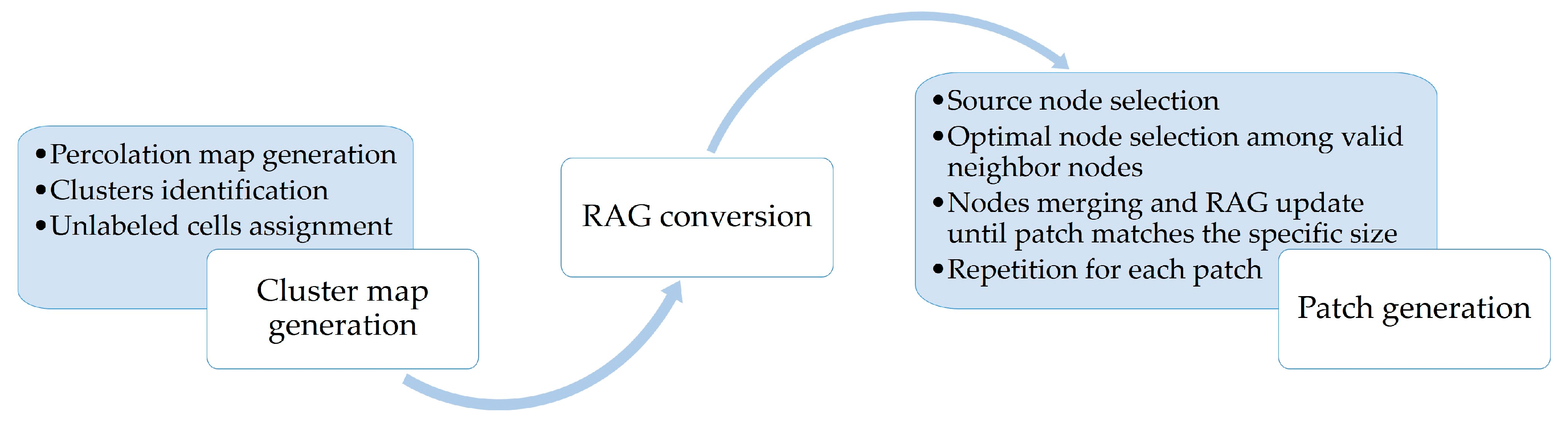
The NLM proposed in this paper is based on a region adjacency graph (RAG), which comprises the following three steps (Figure 1): (1) divide a grid into many clusters based on a percolation map; (2) convert the clusters into an RAG, within which a node records the size and perimeter of the corresponding cluster and an edge records the shared border length between two connected clusters; and (3) generate a patch by merging adjacent nodes to match a specific size and shape until all of the patches have been addressed. The results of the graph-based NLM constitute the spatial patterns of tree species within a square lattice containing L × L cells, where L is the grid dimension.
2.1. Model Parameters
Landscape metrics can be computed at three levels; namely, the landscape level, class level and patch level. Patch-level landscape metrics are generally used as the basis for calculating the other two levels, but are not of great value for understanding the entire landscape pattern [25]. Class-level landscape metrics, including the number of patches (PN) and the mean shape index (MSI), can be calculated from patches of the same tree species and are used to describe the spatial distribution characteristics of different plant types. Our model uses class-level landscape metrics to explicitly control the spatial patterns of each species. The model generates patches of the same species (e.g., spruce) in sequence, and their statistical values of the quantity and shape index are consistent with the given class-level landscape metrics. The component proportion of each tree species is used to describe the composition of the forest landscape, while the PN and MSI are used to quantitatively describe the spatial configuration of each species. The input parameters are described in Table 1. is less than or equal to 1, where the remaining area represents the bare background. The mean patch size is indirectly controlled by the PN when the total area of a tree species is constant. The MSI is a measure of the complexity of the patch shape relative to a regular geometry, which is a circle in our model. The shape of a patch is circular when the MSI is 1; meanwhile, the shape becomes much more complex with increasingly higher MSI values.
2.2. Cluster Map Generation
The first step in our model is the generation of a cluster map, which divides the square lattice into numerous clusters. A percolation map is initially produced, similar to the modified random cluster (MRC) method. Firstly, for each one of the cells, a random number taken from the uniform distribution between 0 and 1 is assigned and compared with the initial probability . If the random value is smaller than , the pixel is marked as black (Figure 2a). Secondly, the clusters composed of black cells are identified and labeled with unique numbers. A set of marked cells that are adjacent on the basis of the 4-neighborhood criteria constitutes a cluster and is uniquely colored (Figure 2b). Finally, in contrast to the MRC method, each unlabeled cell is assigned the label of the cluster closest to that cell (Figure 2c). According to percolation theory, the size of the largest cluster greatly increases and occupies most of the cells spanning the opposite sides of the grid when is close to the percolation threshold (0.5928). To avoid this problem and to separate the clusters evenly, is set to 0.45. A number of irregularly shaped clusters are obtained in this step.
2.3. Conversion of the Cluster Map to an RAG
In this step, the cluster map is converted into a region adjacency graph (RAG), in which a node represents a cluster and an edge between two adjacent nodes represents the neighborhood relationship. We use an edge detection filter to scan each cell within the cluster map from left to right and row by row. The filter examines a central cell and the cells below it and to its right one at a time, which ensures only one check between two adjacent cells (Figure 3). If the label of a neighbor cell is different from that of the central cell, a search operation is performed to check whether an edge exists that connects these two cells in the RAG. An edge with a value of 1 is created if such an edge does not exist; otherwise, the value of the edge is incremented by 1. The value of an edge is the length of the shared border between two connected nodes representing two adjacent clusters. The perimeter of a cluster can be easily calculated by summing all of the edge values linking the cluster node. For example, the perimeter of Cluster 7 is the sum of the border lengths with the six neighboring clusters shown in Figure 4. The size and perimeter of each cluster are recorded as properties within the corresponding node. An additional node property is the species, which is initially set to 0, indicating that the cluster has not been assigned to a tree species.
2.4. Patch Generation by Merging Clusters
In this step, one species is assigned to each node in the RAG generated during the previous step. The objective is to convert a cluster map with a large number of clusters into a class map with n tree species, each of which occupies a proportion of the total area set by the user. The landscapes serving as tree species maps are generated in patches composed of sets of adjacent clusters. A patch grows by merging optimal neighbor nodes while approaching the specified target shape index from a source node; this growth ends when the size of a patch falls within an interval of . The target size and shape index of each patch can be specified from the input parameters:
The selection of the source nodes and the valid neighbor nodes should meet the following conditions:
- source node: a node with a species property of 0 that is not adjacent to nodes of the same species with the currently growing patch.
- valid neighbor nodes: nodes with a species property of 0 adjacent to the source node, the neighboring nodes of which are not connected to nodes of the same species with the currently growing patch.
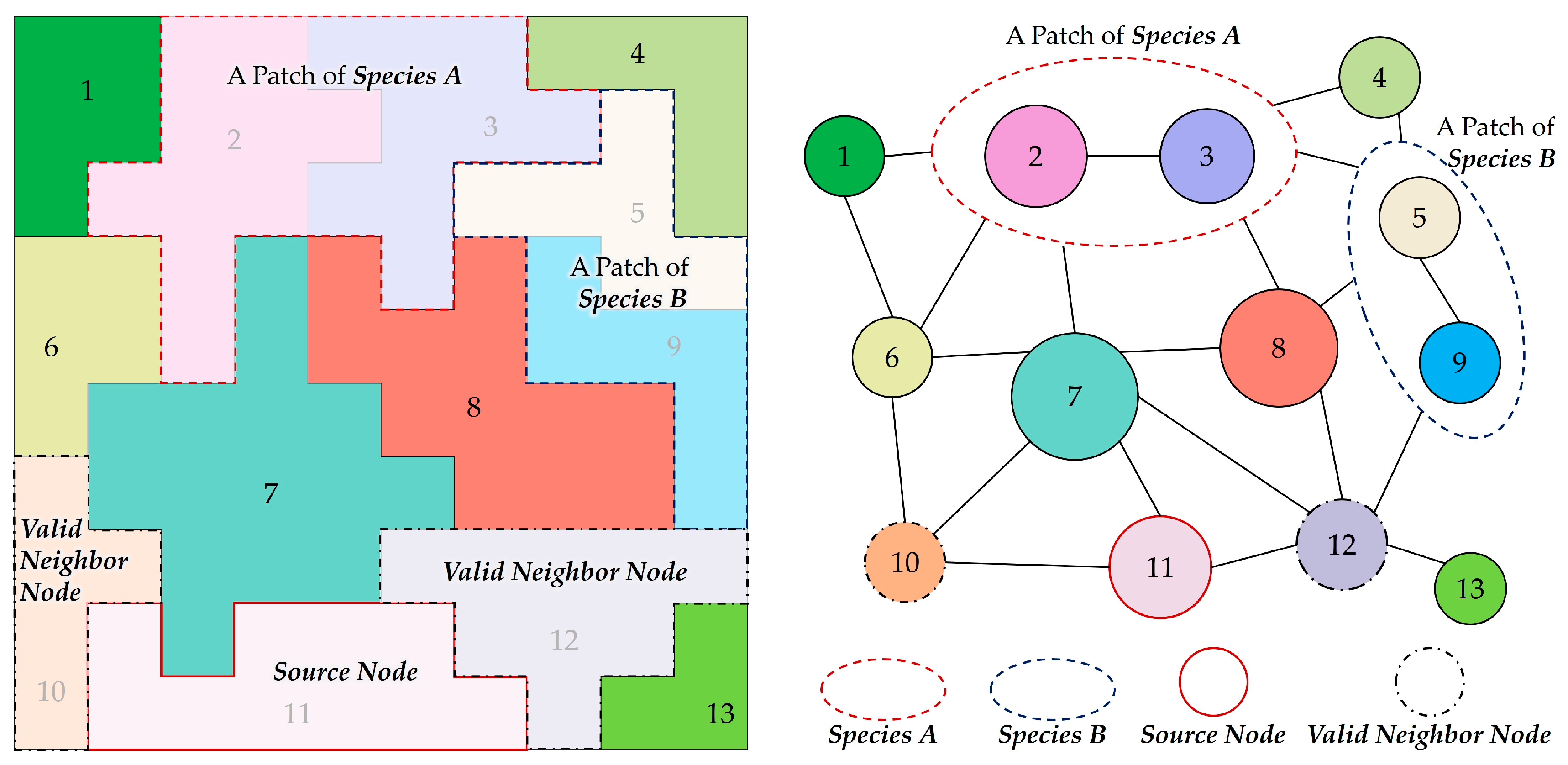
Figure 5 illustrates the selection process in detail. Consider that a patch of Species A is created by combining Cluster 2 and Cluster 3, and that a patch of Species B is created by combining Cluster 5 and Cluster 9. One of the Clusters 10, 11, 12, and 13 can be a source node when generating a patch for Species A, while Clusters 1, 4, 6, 7, and 8 cannot be source nodes. The growing patch will be connected to the existing patch of Species A if an invalid source node is selected, following which the species will be assigned a wrong number of patches. Provided that Cluster 11 is selected as the source node from the above candidates, Cluster 10 and Cluster 12 are valid neighbor nodes that can be merged, while Cluster 7 is not valid, because it is adjacent to a patch of Species A (i.e., the number of patches will be wrong if it is merged).
After the source node is selected and the valid neighbor nodes are subsequently determined, the shape index is calculated for the new cluster consisting of the source node and each valid neighbor node using the following formula, in which and denote the source node and valid neighbor node , respectively, and represents the value of the edge connecting two nodes:
The border will collapse when two neighbor nodes are merged. To obtain the perimeter of the new cluster, the doubled border length should be extracted from the sum of the perimeters of the two nodes. The shape index can be easily calculated by recording the border lengths of neighboring clusters without any additional traversals of the cluster map. An optimal neighbor node is selected to minimize and is merged with the source node. Meanwhile, the label of the merged cluster is recorded within the merged node list stored by the source node. The structure of the RAG should then be updated, because the topological relations change when two nodes are merged together. The properties of the source node are updated with the size and perimeter of the new cluster. This completes an entire cycle of the merge operation, which is repeated until the value of is less than the established threshold. After a patch is finished, the species property of the node should be updated to the species of the patch.
The established thresholds are related to the patch size to avoid an infinite loop when creating a small patch, and thus, the minimum of threshold is set to 50.
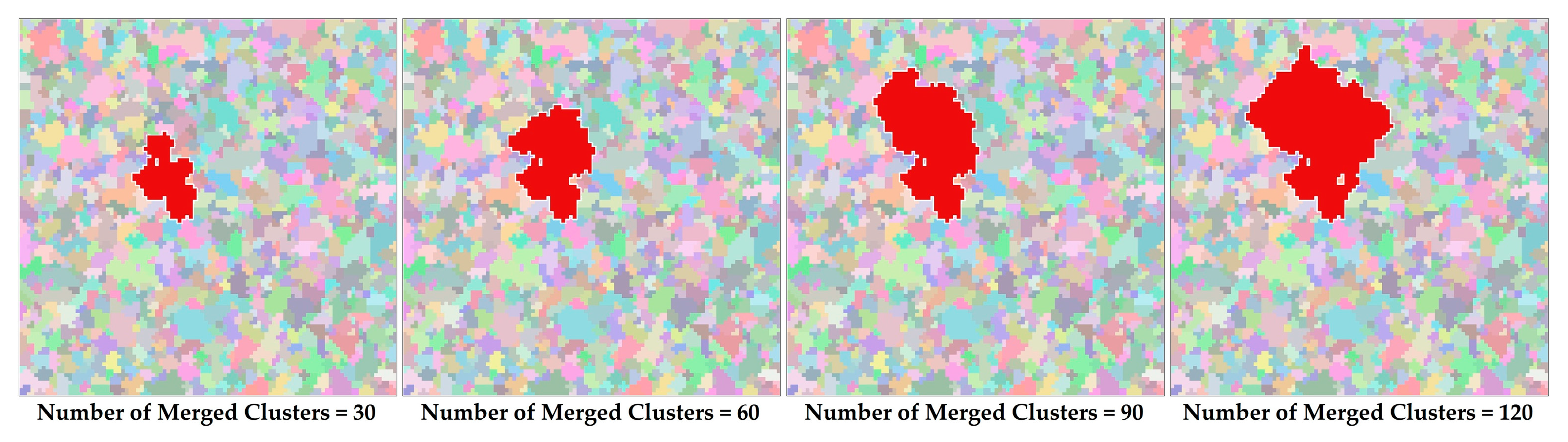
Figure 6 illustrates the generation process of a patch with a of 2.0 in a 100 × 100 grid. A total of 120 nodes are merged during the growth process, and the actual size and shape index are 905 and 1.99, respectively. To minimize the error between the actual and target values and to satisfy the input parameters, namely, the PN and MSI, the deviation in a newly generated patch should be evenly compensated with regard to the patches that have yet to be generated by updating PN and MSI. After all of the patches in each species are finished, the labels of the cells in the cluster map are reassigned according to the merged node list, which provides a mapping from labels to species, and thus, a landscape is generated.
3. Results
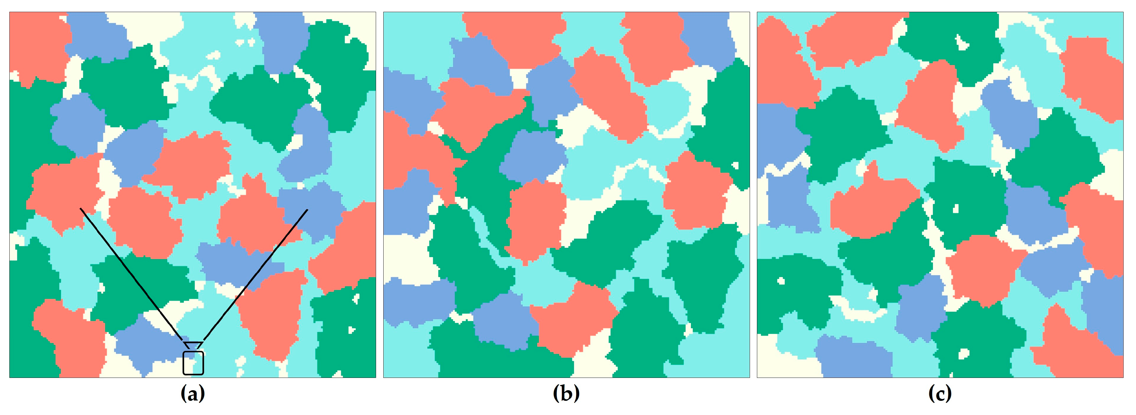
A sample area of 2.5 km × 2.5 km in the Liangshui National Nature Reserve, which is located in middle of Heilongjiang Province, China, is taken as the study area to validate the fitting ability of the proposed NLM. The area is mountainous, and its average altitude is about 400 meters. The tree species distribution of the area is shown in Figure 7. The forest landscape is composed of four tree species (spruce, birch, pine and larch), and the P, PN and MSI of each species can be obtained based on statistics (Table 2) that are then used as model input parameters to synthesize landscapes similar to the study area. Three forest landscape instances (100 × 100 cells) are generated using the graph-based NLM (Figure 8), the actual landscape metrics of which are also shown in Table 2. The patches of pine trees have the highest MSI, and their shapes are much more complex in the sample area. Accordingly, the same distribution characteristics are presented in the generated landscapes, in which the shapes of patches of pine trees twist and turn.
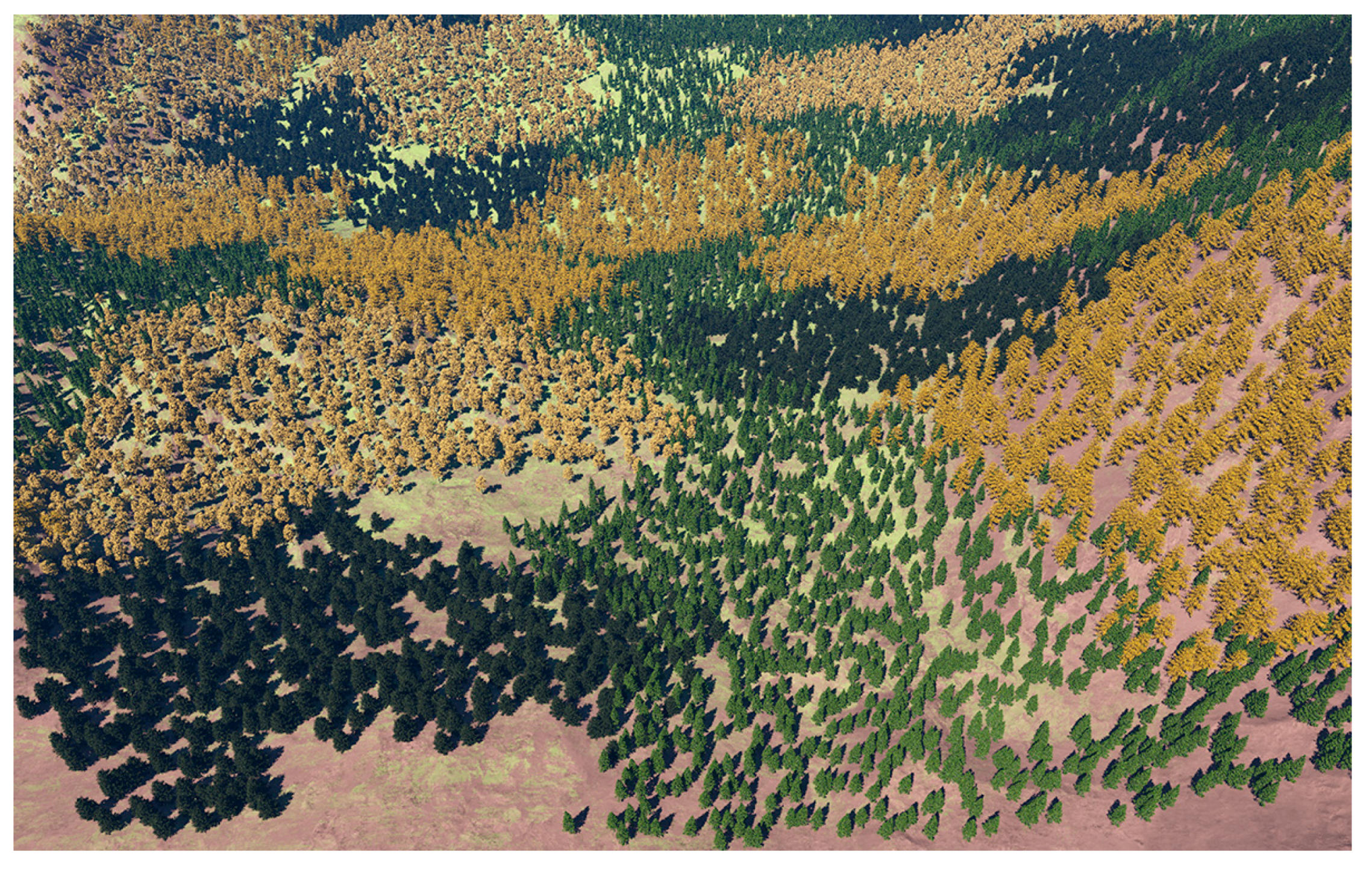
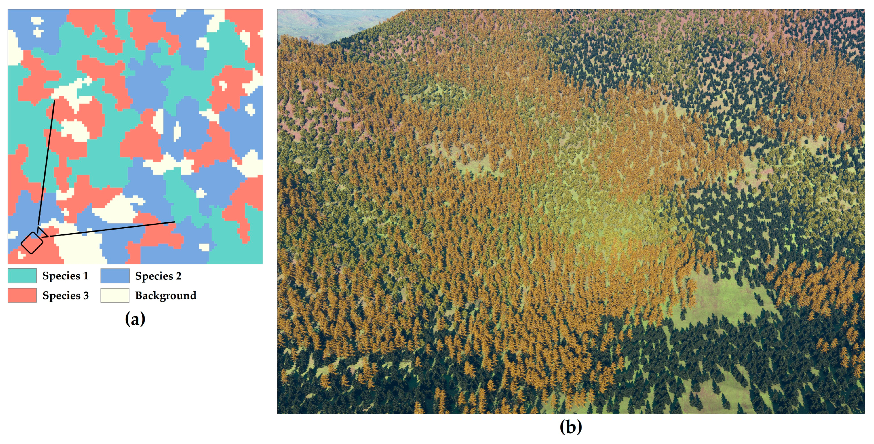
The locations of the seeds are randomly placed, and the species are specified based on the landscapes. To simulate the gradient transitions [36] along the boundaries in the nature scenes, an n × n window is applied to determine the species of each tree through a random assignment taken from the uniform distribution of species proportions in that window. The border transitions are abrupt when n is small, and gentle when n is large. Finally, the tree heights and canopy extents conforming to the statistical features of the species are assigned to the tree. Figure 9 shows the rendering result of tree distributions based on Figure 8a using the Terragen software. The scene depicts a forest landscape during the autumn that is composed of four species of trees. A different virtual forest landscape with three species and its rendering result are shown in Figure 10. The DEM data (30 m resolution) of this area is downloaded from the Geospatial Data Cloud (http://www.gscloud.cn/), a website for free geospatial data. In fact, altitude has a great impact on species distribution, but that is beyond the scope of this paper. The height field is only used for visualization.
4. Discussion
4.1. Error Analysis
The graph-based NLM can generate different instances with similar spatial pattern characteristics controlled by the same input parameters (Figure 8). Both the target values and the actual values of the landscape metrics for each species are listed in Table 2. The PNs of each species are precise and absent errors because the landscapes are produced in units of patches. The errors of , and for three instances fall within of the target value, while is always less than the target value. In addition, the errors of MSIs for spruce, birch and larch fall within , while the error of is larger. This is due to the order of the patch generation, which is sorted according to the MSI values (i.e., from small to large). Many clusters can be merged for the patches that are generated early, and they easily approach the target values. However, less space is available for patches generated later, and they usually grow within the gaps between existing patches of other species or around them, causing the MSI to be large. Thus, patches with large MSI values are arranged for generation last to minimize the errors. As stated above, the possibility exists that only a few neighbor nodes can be merged due to space limitations; thus, growing patches must select the best option among the remaining inappropriate clusters, which deviate from the target shape index. Another situation may occur in which no adjacent cluster is available for merging to accommodate a growing patch (e.g., Cluster 4 in Figure 5), since the remaining space may be split by numerous patches. In this case, the properties of the current patch are recorded and the RAG is restored to the state prior to generation. An additional T attempts are performed until the patch is finished successfully; otherwise, the patch that is the most similar to the target patch is selected. This is why is always less than the target value. Although errors are present within the class-level landscape metrics, the spatial pattern of each species can be clearly distinguished.
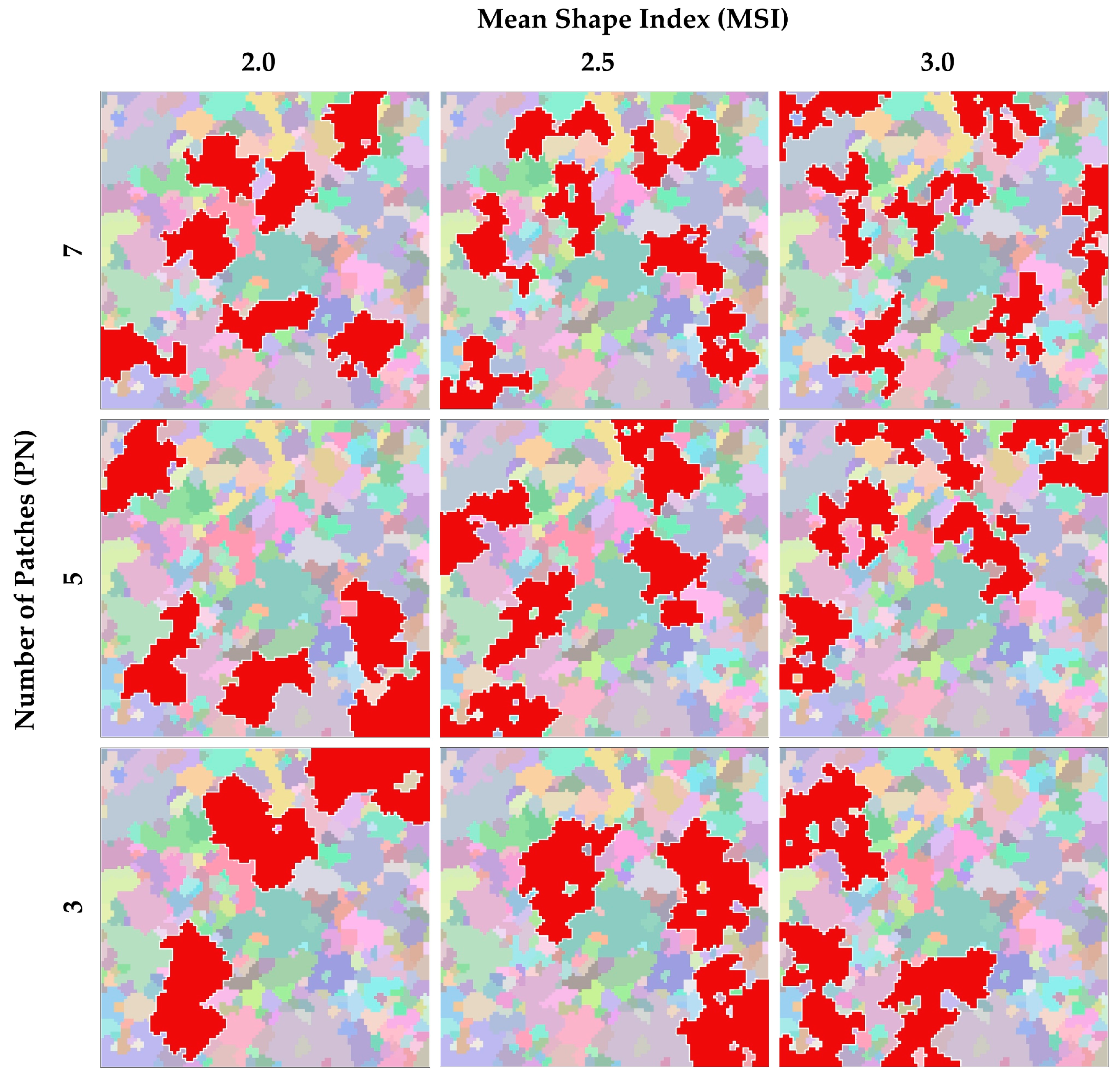
4.2. Controllability of the PN and MSI Parameters
Traditional NLMs cannot separately present the spatial pattern of each species through the use of several landscape-level metrics. In comparison, the proposed model implements a greater number of class-level landscape metrics and exhibits more control over both the PN and the MSI. Figure 11 shows the effects of different PNs and MSIs on the landscape patterns. The red area in each landscape represents a single tree species that takes up 20% of the total area. With an increase in the MSI, the distribution pattern becomes more elongated and complex. The shapes of the patches twist and turn with increasingly higher MSI values, while their shapes are more consolidated when the MSI is low. The PN affects the degree to which the patches are aggregated. With an increasing PN, the distribution pattern becomes more dispersed when the proportion of a particular species is constant.
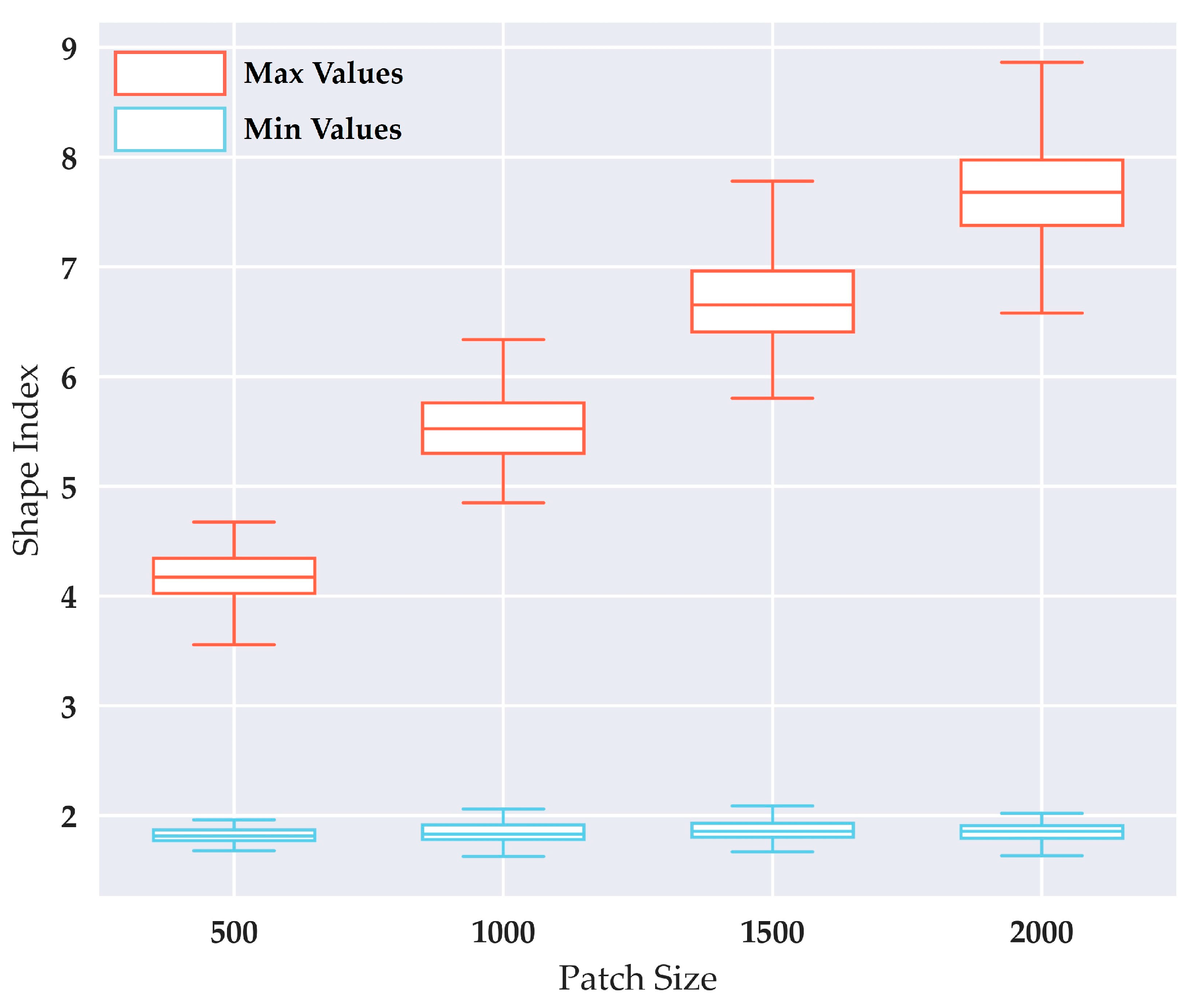
The MSI, which represents the shape complexity of a patch, is an important parameter in our model. This parameter is not set arbitrarily; rather, it should fall within the interval that our model can reasonably fit. To obtain the maximum value of this interval, only one patch is produced by merging a specific node that maximizes the shape index of the merged cluster in every merging operation in step 3. Because of the randomness of the cluster maps, an experimental result is not representative; thus, 100 tests are performed to obtain the range of maximum shape index values. The range of minimum values is similarly obtained. Figure 12 shows the range of maximum and minimum values for a constant patch size. The median maximum value increases with the patch size, because many clusters are more likely to constitute a patch with a high shape complexity. The median minimum value is approximately 1.7, and exhibits no correlation with the patch size. The maximum MSI is set according to the mean patch size. For example, when the mean patch size is approximately 500, an appropriate value of 4.0 is established as the MSI maximum.
4.3. Time Efficiency Analysis
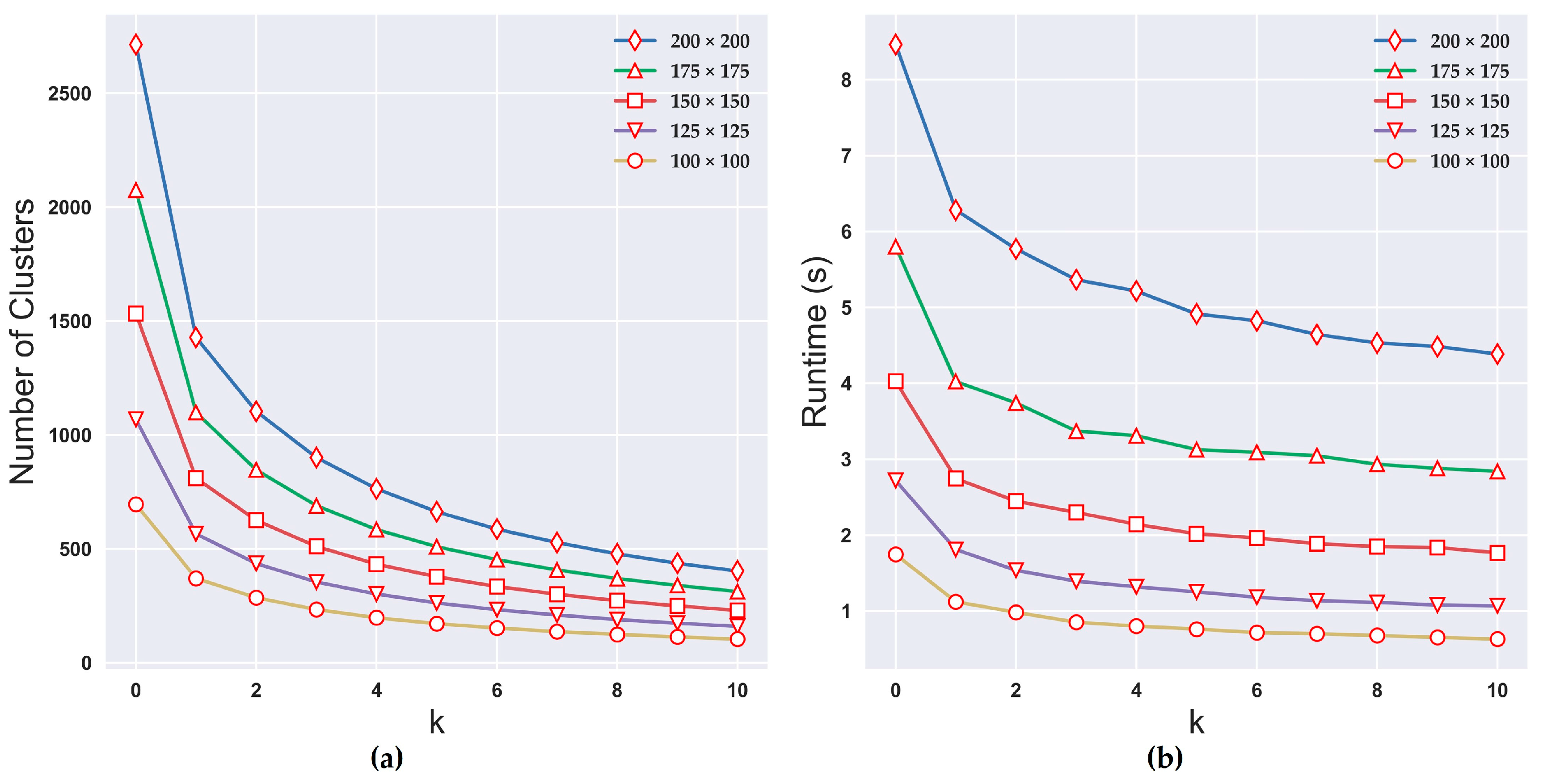
A number of query operations are performed for neighboring nodes in our model. Consequently, the time efficiency is greatly influenced by the number of clusters. There are some clusters containing relatively few cells (Figure 2b) that contribute little to the patch shape. This complicates the RAG and causes a substantial burden on the frequent query operations. In our method, a k value representing the minimum cluster size is used to filter the clusters according to whether their sizes are less than k. If smaller clusters (i.e., with sizes smaller than k) are removed by labeling them as 0 during the clusters identification in the first step, the number of clusters from the percolation map is significantly reduced. Figure 13a demonstrates that the number of clusters (over an average of 100 experiments) decreases as the value of k increases when the grid dimension is constant. The runtime trend (over an average of 100 experiments that produce the same landscapes in Figure 8) with the variations in k is consistent with the number of clusters (Figure 13b). When k = 1, the curve has the steepest drop from k = 0 and the runtime is greatly reduced. Our model is implemented using the Python programming language [37], and the performance is tested on a 2.3 GHz Intel Xeon with 8 GB RAM. The average runtime is less than one second when L = 100 and k ≥ 2. The errors may be larger as the average cluster size rises, although a larger value of k could decrease the runtime. The sizes and shapes of the patches cannot be self-corrected through the iterative merging of small fragments.
5. Conclusions
In this article, we propose a novel graph-based NLM to generate landscapes while reflecting the spatial pattern characteristics of each tree species. The tree distributions are produced through random seeding based on the landscape, and the distribution characteristics of each species can be readily recognized from the final rendered scenes. Compared with other NLMs, our model is advantageously variable and flexible, and can accordingly control various class-level landscape metrics, including the PN and MSI of each species. This is implemented via iterative merging operations from a source node to match the target values of individual patches. The results reveal that the PN parameter can be precisely controlled, while the input proportion and MSI parameters exhibit errors, especially for the patches that are generated last, which constitutes a shortcoming of the proposed model. The graph-based NLM can be employed for not only the generation of vegetation distributions but also other studies in the field of landscape ecology. With the capacity to recreate spatial patterns from real landscapes, the proposed model can help ecologists to study the effects of landscape patterns on ecological processes.
There are several possibilities for future studies. Although the generated landscapes conform to the given class-level landscape metrics, visual inconformity exists compared with the sample area. It is difficult to represent the shapes of patches by shape index only. Other metrics, such as bounding box aspect-ratio of patch and proportion of bounding box area, can be included in the model to enhance the controllability of patch shape [34]. Additionally, our model ignores the underlying ecosystems (e.g., shrubs, grasses and younger trees, which are all in competition), considering patches to consist of a single tree species. This can be improved by extension from 2D NLM to 3D NLM, which considers the height of forests.
NLMs can simulate and replicate a given spatial pattern; however, most NLMs, including our proposed model, do not consider non-biological environmental factors (e.g., the elevation, slope and aspect) affecting plant distributions. For example, some species are not suitable for survival at certain altitudes, and tree growth is weak on steep slopes. Subsequent studies could be conducted to integrate the terrain encoded via a digital elevation model (DEM) or a triangular irregular network (TIN) model. The suitability of a cluster for each individual species can be evaluated according to weighted abiotic factors and should be considered when selecting the optimal merging node.
Acknowledgments
This study was supported by the National Natural Science Foundation of China (Grant No. 41371365).
Author Contributions
Jiaqi Li designed and implemented the proposed model and wrote part of the paper; Xiaoyan Gu wrote part of the paper and made the figures; Xinchi Li implemented the model and performed the experiments; Junzhong Tan conceived and designed the proposed model and analyzed the results; Jiangfeng She conceived and designed the proposed model and revised the manuscript.
Conflicts of Interest
The authors declare no conflicts of interest.
References
- Deussen, O.; Hanrahan, P.; Lintermann, B.; Měch, R.; Pharr, M.; Prusinkiewicz, P. Realistic Modeling and Rendering of Plant Ecosystems. In Proceedings of the 25th Annual Conference on Computer Graphics and Interactive Techniques, Orlando, FL, USA, 19–24 July 1998; Association for Computing Machinery (ACM): New York, NY, USA; pp. 275–286. [Google Scholar]
- Takenaka, T.; Okabe, A. Development of the seed scattering system for computational landscape design. Int. J. Archit. Comput. 2011, 9, 421–436. [Google Scholar] [CrossRef]
- Chou, C.-Y.; Song, B.; Hedden, R.L.; Williams, T.M.; Culin, J.D.; Post, C.J. Three-dimensional landscape visualizations: New technique towards wildfire and forest bark beetle management. Forests 2010, 1, 82–98. [Google Scholar] [CrossRef]
- Pradal, C.; Boudon, F.; Nouguier, C.; Chopard, J.; Godin, C. Plantgl: A python-based geometric library for 3d plant modelling at different scales. Graph. Model. 2009, 71, 1–21. [Google Scholar] [CrossRef] [Green Version]
- Bruneton, E.; Neyret, F. Real-Time Realistic Rendering and Lighting of Forests. Comput. Graph. Forum 2012, 31, 373–382. [Google Scholar] [CrossRef]
- Santoro, F.; Tarantino, E.; Figorito, B.; Gualano, S.; D’Onghia, A.M. A tree counting algorithm for precision agriculture tasks. Int. J. Digit. Earth 2013, 6, 94–102. [Google Scholar] [CrossRef]
- Andújar, C.; Chica, A.; Vico, M.A.; Moya, S.; Brunet, P. Inexpensive reconstruction and rendering of realistic roadside landscapes. Comput. Graph. Forum 2014, 33, 101–117. [Google Scholar] [CrossRef] [Green Version]
- Dutta, D.; Wang, K.; Lee, E.; Goodwell, A.; Woo, D.K.; Wagner, D.; Kumar, P. Characterizing vegetation canopy structure using airborne remote sensing data. IEEE Trans. Geosci. Remote Sens. 2017, 55, 1160–1178. [Google Scholar] [CrossRef]
- Silva, C.A.; Hudak, A.T.; Vierling, L.A.; Loudermilk, E.L.; O’Brien, J.J.; Hiers, J.K.; Jack, S.B.; Gonzalez-Benecke, C.; Lee, H.; Falkowski, M.J.; et al. Imputation of individual longleaf pine (pinus palustris mill.) tree attributes from field and lidar data. Can. J. Remote Sens. 2016, 42, 554–573. [Google Scholar] [CrossRef]
- Trochta, J.; Krucek, M.; Vrska, T.; Kral, K. 3d forest: An application for descriptions of three-dimensional forest structures using terrestrial lidar. PLoS ONE 2017, 12, e0176871. [Google Scholar] [CrossRef] [PubMed]
- Abegg, M.; Kükenbrink, D.; Zell, J.; Schaepman, M.E.; Morsdorf, F. Terrestrial laser scanning for forest inventories—Tree diameter distribution and scanner location impact on occlusion. Forests 2017, 8, 184. [Google Scholar] [CrossRef]
- Samavati, F.; Runions, A. Interactive 3d content modeling for digital earth. Vis. Comput. 2016, 32, 1293–1309. [Google Scholar] [CrossRef]
- Berger, U.; Hildenbrandt, H. A new approach to spatially explicit modelling of forest dynamics: Spacing, ageing and neighbourhood competition of mangrove trees. Ecol. Model. 2000, 132, 287–302. [Google Scholar] [CrossRef]
- Ch’Ng, E. Model resolution in complex systems simulation: Agent preferences, behavior, dynamics and n-tiered networks. Simulation 2013, 89, 635–659. [Google Scholar] [CrossRef]
- Lane, B.; Prusinkiewicz, P. Generating spatial distributions for multilevel models of plant communities. In Proceedings of the Graphics Interface, Calgary, AB, Canada, 27–29 May 2002; Canadian Human-Computer Communications Society (CHCCS): Mississauga, ON, Canada, 2002; pp. 69–87. [Google Scholar]
- Zamuda, A.; Brest, J. Environmental framework to visualize emergent artificial forest ecosystems. Inf. Sci. 2013, 220, 522–540. [Google Scholar] [CrossRef]
- Bradbury, G.A.; Subr, K.; Koniaris, C.; Mitchell, K.; Weyrich, T. Guided ecological simulation for artistic editing of plant distributions in natural scenes. J. Comput. Graph. Tech. 2015, 4, 28–53. [Google Scholar]
- Gain, J.; Long, H.; Cordonnier, G.; Cani, M.P. Ecobrush: Interactive control of visually consistent large-scale ecosystems. Comput. Graph. Forum 2017, 36, 63–73. [Google Scholar] [CrossRef]
- Soares-Filho, B.S.; Cerqueira, G.C.; Pennachin, C.L. Dinamica—A stochastic cellular automata model designed to simulate the landscape dynamics in an amazonian colonization frontier. Ecol. Model. 2002, 154, 217–235. [Google Scholar] [CrossRef]
- Scheller, R.M.; Domingo, J.B.; Sturtevant, B.R.; Williams, J.S.; Rudy, A.; Gustafson, E.J.; Mladenoff, D.J. Design, development, and application of landis-ii, a spatial landscape simulation model with flexible temporal and spatial resolution. Ecol. Model. 2007, 201, 409–419. [Google Scholar] [CrossRef]
- Alsweis, M.; Deussen, O. Wang-tiles for the simulation and visualization of plant competition. In Advances in Computer Graphics; Springer: Berlin/Heidelberg, Germany, 2006; pp. 1–11. [Google Scholar]
- Weier, M.; Hinkenjann, A.; Demme, G.; Slusallek, P. Generating and rendering large scale tiled plant populations. J. Virtual Real. Broadcast. 2013, 10. [Google Scholar] [CrossRef]
- Öztireli, A.C.; Gross, M. Analysis and synthesis of point distributions based on pair correlation. ACM Trans. Graph. 2012, 31, 170. [Google Scholar] [CrossRef]
- Emilien, A.; Vimont, U.; Cani, M.-P.; Poulin, P.; Benes, B. Worldbrush: Interactive example-based synthesis of procedural virtual worlds. ACM Trans. Graph. 2015, 34, 106. [Google Scholar] [CrossRef] [Green Version]
- Turner, M.G.; Gardner, R.H.; O’neill, R.V. Landscape Ecology in Theory and Practice; Springer: Berlin/Heidelberg, Germany, 2001; Volume 401. [Google Scholar]
- Houet, T.; Schaller, N.; Castets, M.; Gaucherel, C. Improving the simulation of fine-resolution landscape changes by coupling top-down and bottom-up land use and cover changes rules. Int. J. Geogr. Inf. Sci. 2014, 28, 1848–1876. [Google Scholar] [CrossRef]
- Lustig, A.; Stouffer, D.B.; Roigé, M.; Worner, S.P. Towards more predictable and consistent landscape metrics across spatial scales. Ecol. Indic. 2015, 57, 11–21. [Google Scholar] [CrossRef]
- Gardner, R.H.; Milne, B.T.; Turnei, M.G.; O’Neill, R.V. Neutral models for the analysis of broad-scale landscape pattern. Landsc. Ecol. 1987, 1, 19–28. [Google Scholar] [CrossRef]
- O’neill, R.; Gardner, R.; Turner, M. A hierarchical neutral model for landscape analysis. Landsc. Ecol. 1992, 7, 55–61. [Google Scholar] [CrossRef]
- Gardner, R.H. Rule: Map generation and a spatial analysis program. In Landscape Ecological Analysis: Issues and Applications; Springer: Berlin/Heidelberg, Germany, 1999; pp. 280–303. [Google Scholar]
- Saura, S.; Martínez-Millán, J. Landscape patterns simulation with a modified random clusters method. Landsc. Ecol. 2000, 15, 661–678. [Google Scholar] [CrossRef]
- Gaucherel, C. Neutral models for polygonal landscapes with linear networks. Ecol. Model. 2008, 219, 39–48. [Google Scholar] [CrossRef]
- Li, X.; He, H.S.; Wang, X.; Bu, R.; Hu, Y.; Chang, Y. Evaluating the effectiveness of neutral landscape models to represent a real landscape. Landsc. Urban Plan. 2004, 69, 137–148. [Google Scholar] [CrossRef]
- Slager, C.T.J.; de Vries, B. Landscape generator: Method to generate landscape configurations for spatial plan-making. Comput. Environ. Urban Syst. 2013, 39, 1–11. [Google Scholar] [CrossRef]
- Van Strien, M.J.; Slager, C.T.; Vries, B.; Grêt-Regamey, A. An improved neutral landscape model for recreating real landscapes and generating landscape series for spatial ecological simulations. Ecol. Evol. 2016, 6, 3808–3821. [Google Scholar] [CrossRef] [PubMed]
- Danz, N.P.; Frelich, L.E.; Reich, P.B.; Niemi, G.J. Do vegetation boundaries display smooth or abrupt spatial transitions along environmental gradients? Evidence from the prairie-forest biome boundary of historic minnesota, USA. J. Veg. Sci. 2013, 24, 1129–1140. [Google Scholar] [CrossRef]
- Oliphant, T.E. Python for scientific computing. Comput. Sci. Eng. 2007, 9. [Google Scholar] [CrossRef]
Figure 1.
The flow diagram of our method.

Figure 2.
(a) A percolation map. (b) The clusters identified based on the 4-neighborhood criteria. (c) A cluster map with assigned unlabeled cells.
Figure 2.
(a) A percolation map. (b) The clusters identified based on the 4-neighborhood criteria. (c) A cluster map with assigned unlabeled cells.
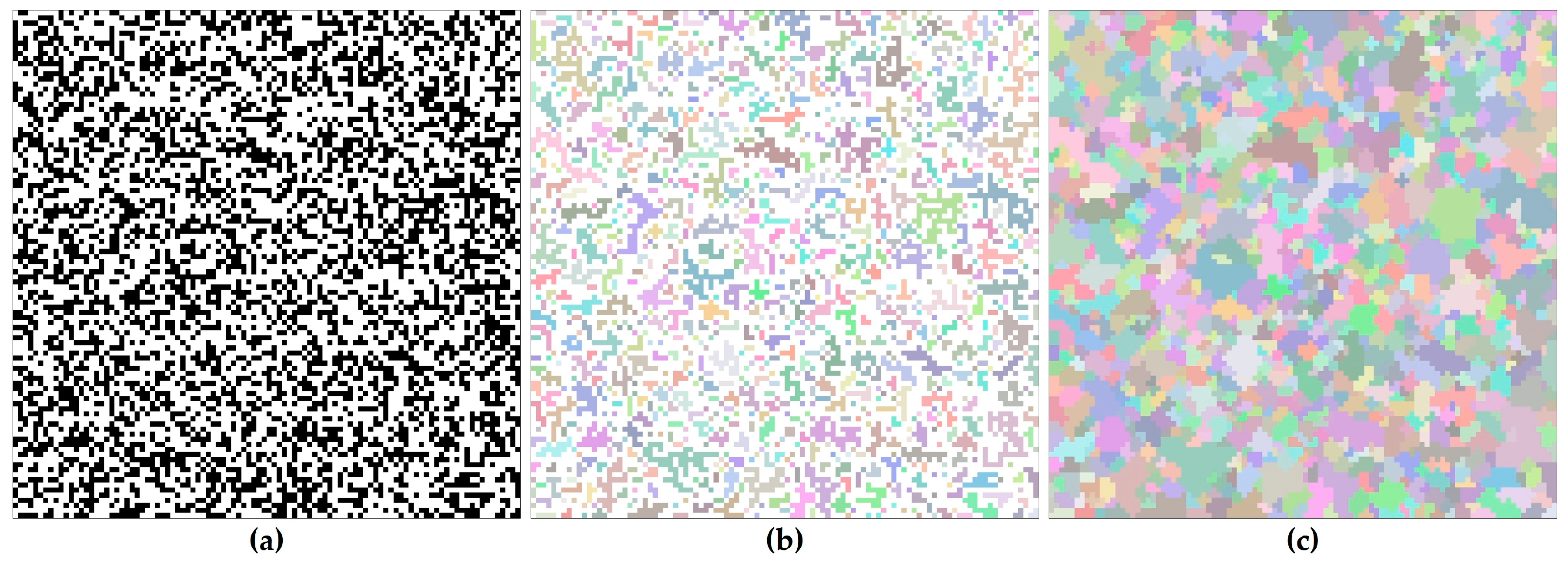
Figure 3.
The neighborhood relation between Cluster 2 and Cluster 7 is detected for the first time, and the corresponding edge is created in the RAG.
Figure 3.
The neighborhood relation between Cluster 2 and Cluster 7 is detected for the first time, and the corresponding edge is created in the RAG.
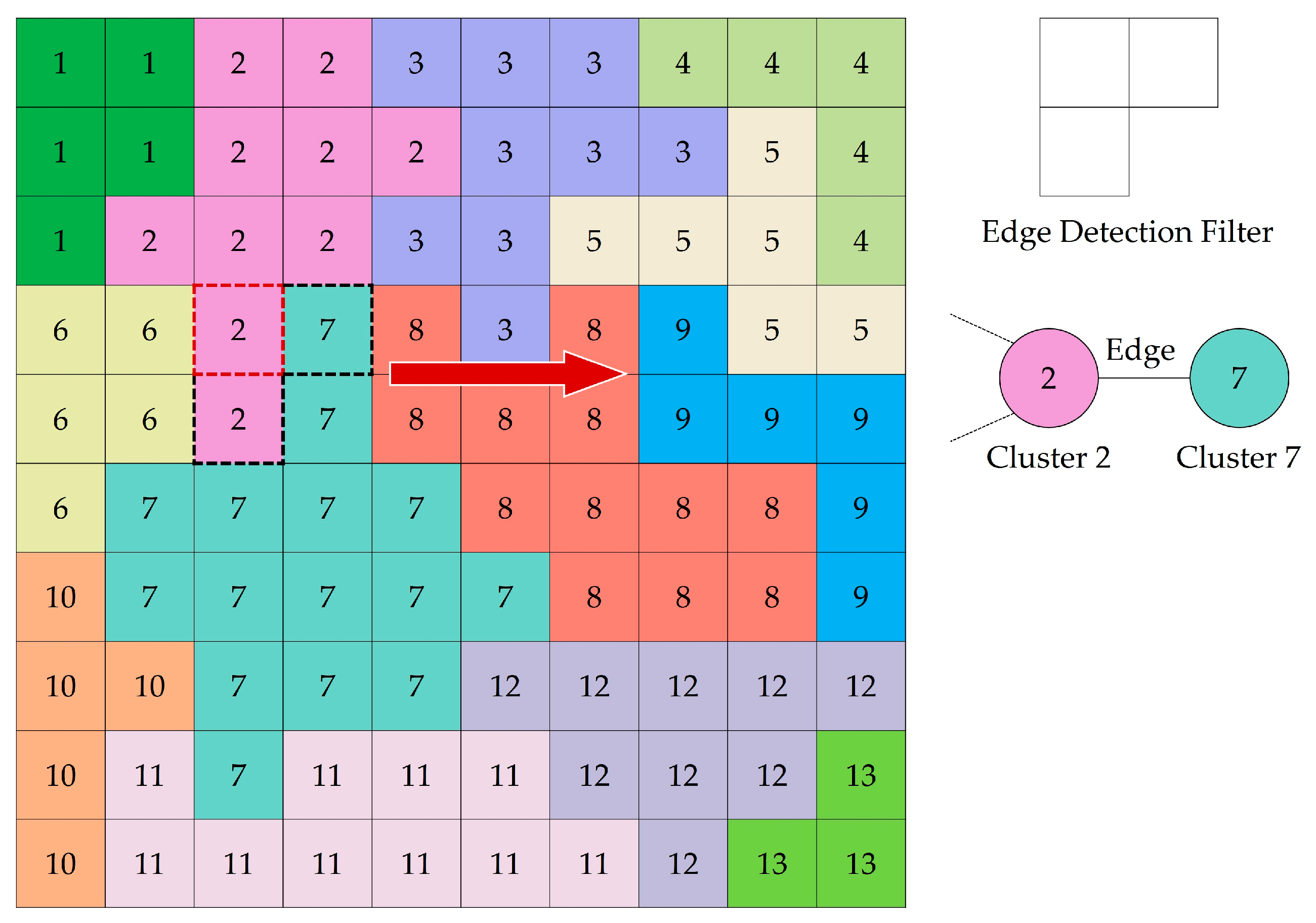
Figure 4.
The RAG converted from the cluster map shown in Figure 3.
Figure 4.
The RAG converted from the cluster map shown in Figure 3.
Figure 5.
The selection of the source node and of the valid neighbor nodes.

Figure 6.
Panels demonstrating that the size of the patch may substantially increase at certain growth steps due to the randomness and irregularity of the cluster.
Figure 6.
Panels demonstrating that the size of the patch may substantially increase at certain growth steps due to the randomness and irregularity of the cluster.

Figure 7.
A 2.5 km × 2.5 km sample plot in the Liangshui National Nature Reserve, Heilongjiang Province, China.
Figure 7.
A 2.5 km × 2.5 km sample plot in the Liangshui National Nature Reserve, Heilongjiang Province, China.
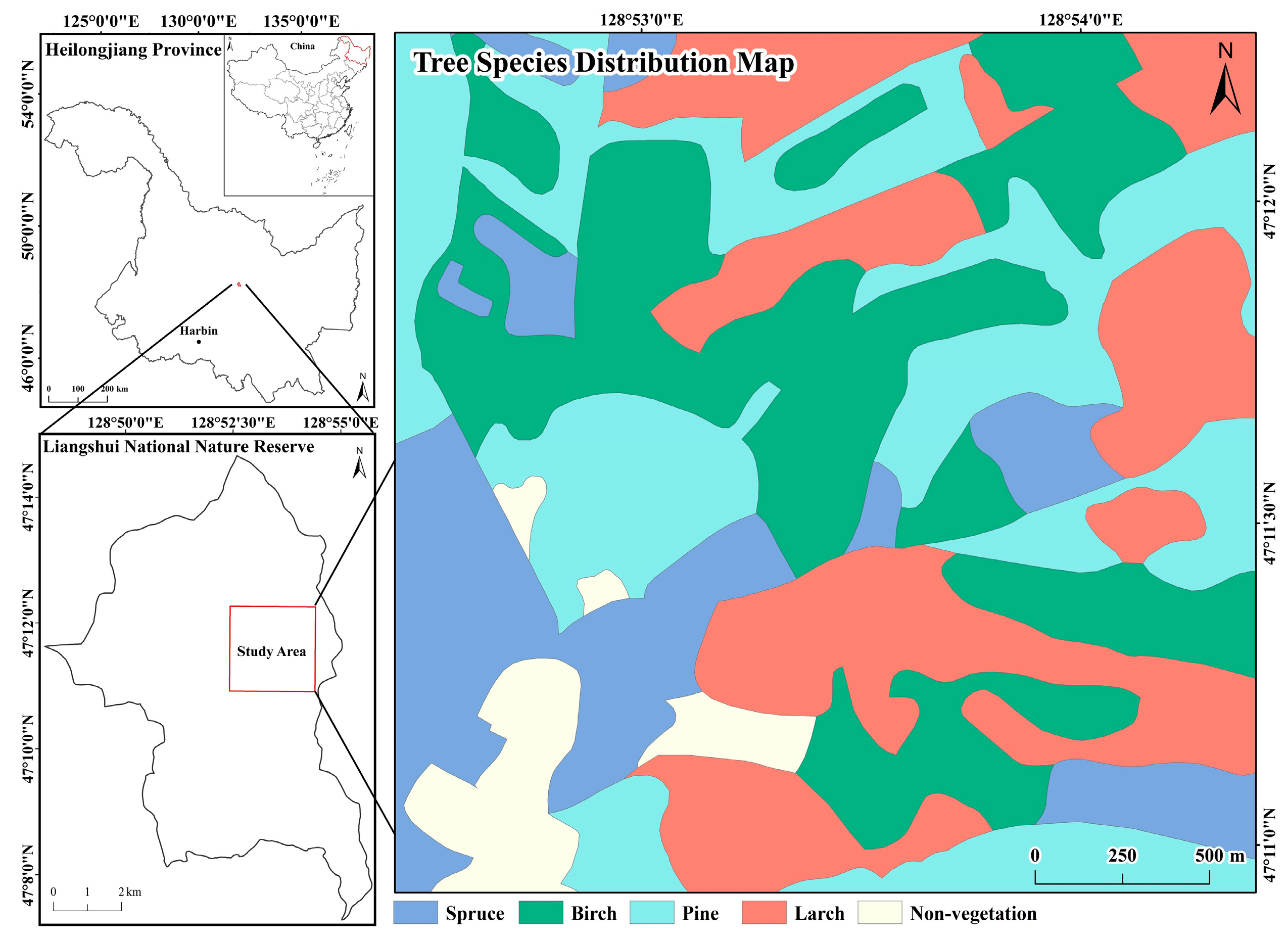
Figure 8.
(a), (b) and (c) are three forest landscape instances generated by the proposed NLM that have similar spatial patterns to the study area. Each instance has 100 × 100 cells and each cell represents a 25 m × 25 m square.
Figure 8.
(a), (b) and (c) are three forest landscape instances generated by the proposed NLM that have similar spatial patterns to the study area. Each instance has 100 × 100 cells and each cell represents a 25 m × 25 m square.

Figure 9.
The rendering result of tree distributions based on Figure 8a.
Figure 9.
The rendering result of tree distributions based on Figure 8a.

Figure 10.
(a) A virtual forest landscape with the following input: = = = 30%, = 5, = 10, = 15, = 2.5 and = = 2.0. (b) The rendering result of tree distribution based on panel (a).
Figure 10.
(a) A virtual forest landscape with the following input: = = = 30%, = 5, = 10, = 15, = 2.5 and = = 2.0. (b) The rendering result of tree distribution based on panel (a).

Figure 11.
The generated landscapes with different PNs and MSIs.

Figure 12.
The distribution of maximum and minimum shape index values from 100 tests with a constant patch size.
Figure 12.
The distribution of maximum and minimum shape index values from 100 tests with a constant patch size.

Figure 13.
(a) The number of clusters as a function of k. (b) The runtime as a function of k.

Table 1.
The model parameters and their formulas.
| Landscape Metric | Variable Name | Formula | Value Range |
|---|---|---|---|
| Landscape proportion | 0.0~1.0 | ||
| Number of patches | Integers (≥1) | ||
| Mean shape index | ≥1.0 |
(i = landscape component, j = patch instance; = area of instance j in species i; = perimeter of instance j in species i; A = L × L).
Table 2.
A comparison between the target values and actual values of the landscape metrics for each tree species.
Table 2.
A comparison between the target values and actual values of the landscape metrics for each tree species.
| Tree Species | Landscape Metric | Target Value | Figure 8a | Figure 8b | Figure 8c |
|---|---|---|---|---|---|
| Spruce | P | 15.8% | 15.9% | 15.9% | 15.9% |
| PN | 8 | 8 | 8 | 8 | |
| MSI | 1.51 | 1.60 | 1.54 | 1.57 | |
| Birch | P | 27.6% | 27.9% | 27.9% | 27.9% |
| PN | 7 | 7 | 7 | 7 | |
| MSI | 1.74 | 1.79 | 1.83 | 1.75 | |
| Pine | P | 26.7% | 24.3% | 23.6% | 23.8% |
| PN | 7 | 7 | 7 | 7 | |
| MSI | 2.20 | 2.35 | 2.29 | 2.43 | |
| Larch | P | 24.4% | 24.0% | 23.9% | 24.0% |
| PN | 8 | 8 | 8 | 8 | |
| MSI | 1.56 | 1.62 | 1.65 | 1.56 |
© 2018 by the authors. Licensee MDPI, Basel, Switzerland. This article is an open access article distributed under the terms and conditions of the Creative Commons Attribution (CC BY) license (http://creativecommons.org/licenses/by/4.0/).
Share and Cite
MDPI and ACS Style
Li, J.; Gu, X.; Li, X.; Tan, J.; She, J. Procedural Generation of Large-Scale Forests Using a Graph-Based Neutral Landscape Model. ISPRS Int. J. Geo-Inf. 2018, 7, 127. https://doi.org/10.3390/ijgi7030127
AMA Style
Li J, Gu X, Li X, Tan J, She J. Procedural Generation of Large-Scale Forests Using a Graph-Based Neutral Landscape Model. ISPRS International Journal of Geo-Information. 2018; 7(3):127. https://doi.org/10.3390/ijgi7030127
Chicago/Turabian StyleLi, Jiaqi, Xiaoyan Gu, Xinchi Li, Junzhong Tan, and Jiangfeng She. 2018. "Procedural Generation of Large-Scale Forests Using a Graph-Based Neutral Landscape Model" ISPRS International Journal of Geo-Information 7, no. 3: 127. https://doi.org/10.3390/ijgi7030127
Note that from the first issue of 2016, this journal uses article numbers instead of page numbers. See further details here.