Revealing Recurrent Urban Congestion Evolution Patterns with Taxi Trajectories

School of Transportation Science and Engineering, Harbin Institute of Technology, Harbin 150090, China
*
Authors to whom correspondence should be addressed.
ISPRS Int. J. Geo-Inf. 2018, 7(4), 128; https://doi.org/10.3390/ijgi7040128
Submission received: 4 February 2018
/
Revised: 10 March 2018
/
Accepted: 17 March 2018
/
Published: 21 March 2018
(This article belongs to the Special Issue Geospatial Big Data and Urban Studies)
Abstract
:Urban congestion can be classified into two types: Recurrent Congestion (RC) and Non-Recurrent Congestion (NRC). RC is more regular than NRC, having fixed and long-standing patterns. Mining urban recurrent congestion evolution patterns can assist with congestion cause analysis and the creation of alleviating strategies. Most existing methods for analyzing urban congestion patterns are based on traditional traffic detector data, which is inflexible and expensive. Additionally, prior research primarily focused on the microscopic model, which simulated congestion propagation based on theoretical models and hypothetical networks. As such, most previous models and methods are difficult to apply to real case scenarios. Therefore, we investigated recurrent congestion patterns by mining historical taxi trajectory data that were collected in Harbin, China. A three-step method is proposed to reveal urban recurrent congestion evolution patterns. Firstly, a grid-based congestion detection method is presented by calculating the change in taxi global positioning system (GPS) trajectory patterns. Secondly, a customized cluster algorithm is applied to measure the recurrent congestion area. Finally, a series of indicators are proposed to reflect RC evolution patterns. A case study was competed in the Harbin urban area to evaluate the main methods. Finally, RC cause analysis and alleviating strategy are discussed. The results study are expected to provide a better understanding of urban RC evolution patterns.
1. Introduction
Recurrent congestion (RC) and Non-Recurrent Congestion (NRC) are two typical types of congestion occurring in urban areas [1]. RC is usually caused by insufficient traffic capacity, excess travel demand, and poor signal control [2,3], to name a few. This type of congestion is regular with typical fixed features, such as having the same generating period, similar spatio-temporal influence scope, duration, etc. [4]. Compared with NRC, RC has a more deleterious effect on the travel time of urban commuters and travelers. Revealing recurrent congestion patterns can help city traffic managers improve signal controllers [5] and urban planners rebuild inferior traffic infrastructures [6], to further alleviate urban recurrent congestion [7].
With the adoption of location-based services (LBS), increasing amounts of multiple-source locating information can be obtained in a city. For example, an increasing number of taxi vehicles have been equipped with GPS modules, so large amounts of taxi GPS data can be collected. In China, taxis are part of public transit, with large numbers of vehicles travelling the urban road network at all times. For example, more than 13,000 taxis operate in Harbin, China, and most of the vehicles are equipped with a GPS module [8]. With a sampling frequency of 30 s, almost 30 million GPS records are obtained every 24 h for managing and operating the taxis. These locating data can reflect the traffic state of the urban environment. Since the late 2000s, a broad range of transportation research has been conducted based on taxi trajectory data, such as building a taxi recommender system [9], predicting link and route travel time [10], and detecting urban traffic congestion [11]. In contrast to traditional traffic detectors, such as loops, microwaves, and video detectors, using taxi GPS data has the obvious advantages of mobility, extensive range coverage, and being inexpensive [12]. Therefore, using taxi GPS trajectory data to study urban RC patterns is reasonable and valid, and the method can be widely applied at a lower cost in comparison with methods based on traditional traffic detectors.
Many existing studies have been completed on urban congestion evolution patterns, and most were based on microscopic traffic flow models, including a cell transmission model (CTM) [13] and a car-following model [14]. For example, Zhang et al. [15] proposed a bi-level programming model based on CTM to investigate the spatio-temporal distribution of traffic flow and the location of variable message signs (VMS) under non-recurrent congestion conditions. Chu et al. [16] proposed a modified CTM (MCTM) to depict the temporal-spatial evolution of traffic congestion on urban freeways. Yang et al. [17] used the MCTM model to investigate the traffic congestion formation and diffusion process due to road capacity drop-down after traffic incidents. Additionally, some studies used car-following models to demonstrate urban congestion evolution patterns. For example, Chen et al. [18] presented a behavioral car-following model based on empirical trajectory data that was able to reproduce spontaneous congestion formation and the ensuing propagation of stop-and-go waves in traffic. Zhu et al. [19] used an enhanced car-following model to estimate delay and emissions for urban signalized intersections. Papathanasopoulou and Antoniou [20] presented an innovative methodological framework based on a data-driven approach to estimate car-following models, which could be used for measuring congestion evolution patterns. Besides, some studies proposed a congestion pattern measuring model based on Dynamic Bayesian Network [21] and other machine learning methods.
These studies have provided valuable insights into urban congestion patterns. However, few studies have focused on urban recurrent congestion patterns. Compared with NRC, RC has more regular patterns, such as fixed periodicity, frequency, and fixed co-occurrence. Additionally, most existing studies used the microscopic traffic flow model to depict urban congestion evolution patterns. These studies simulated congestion propagation based on the theoretical model and hypothetical two-way grid network, which complicated the application of these theories and methods to real life scenarios. In addition, to the best of our knowledge, few studies researched recurrent congestion evolution patterns on a macroscopic level. Therefore, we modeled urban recurrent congestion patterns based on taxi GPS trajectory data at a macroscopic level.
The primary purpose of this study is to present an effective method to explore the RC pattern in an urban area. We had three additional auxiliary goals: to develop an urban congestion detection method based on GPS data at the grid level, to discover the RC area, and to illustrate the RC patterns.
The remainder of this paper is organized as follows: Section 2 introduces GPS trajectory data and the study area with divided grids, and also presents the main methods, including detecting grid congestion, discovering the RC area, and measuring the RC evolution patterns. Section 3 presents the experiment for the main methods and discusses the results, and Section 4 provides our conclusions.
2. Materials and Methods
2.1. Data Collection
Generally speaking, taxi GPS data contain information such as GPS device identification (ID) including taxi ID, location information (i.e., latitude and longitude), timestamp, instantaneous velocity, and direction [22]. In this paper, taxi ID, latitude, longitude, timestamp, and instantaneous velocity were required for measuring the taxi trajectory pattern. In this section, using Harbin taxi GPS data as an example, details about the data are as follows.
Due to the high latitude location, the winter in Harbin lasts from November to March, for a total of 5 months [23]. In winter, the snowy weather and snow accumulation on the road strongly affects city travelers, aggravating urban congestion. As such, we conducted our study during the winter of 2015. Since over 20 million GPS records are created in one day, 5 weeks corresponding to the 5 months were chosen as the sampling period. The GPS data’s sampling rate is 30 s, and the total number of samples for the 25 days was 506 million. Table 1 illustrates a sample Harbin taxi GPS record.
In this paper, oracle 11 g was used to manage the GPS data sets, and ArcGIS 10.0 was used for the GPS interface to manipulate and visualize the GPS data. In addition, the core of the analytical inspection and graphics were fully executed in the R 3.3.3 environment.
2.2. Study Area
Taxi vehicles usually travel around the road network in an urban area. We chose a study area located within the urban area to ensure sufficient taxi GPS locating data would be obtained. Besides, the urban area should be divided into equal-sized grids, which is very simple and easy to implement [22]. In this section, the Harbin urban area was divided into grids as an example.
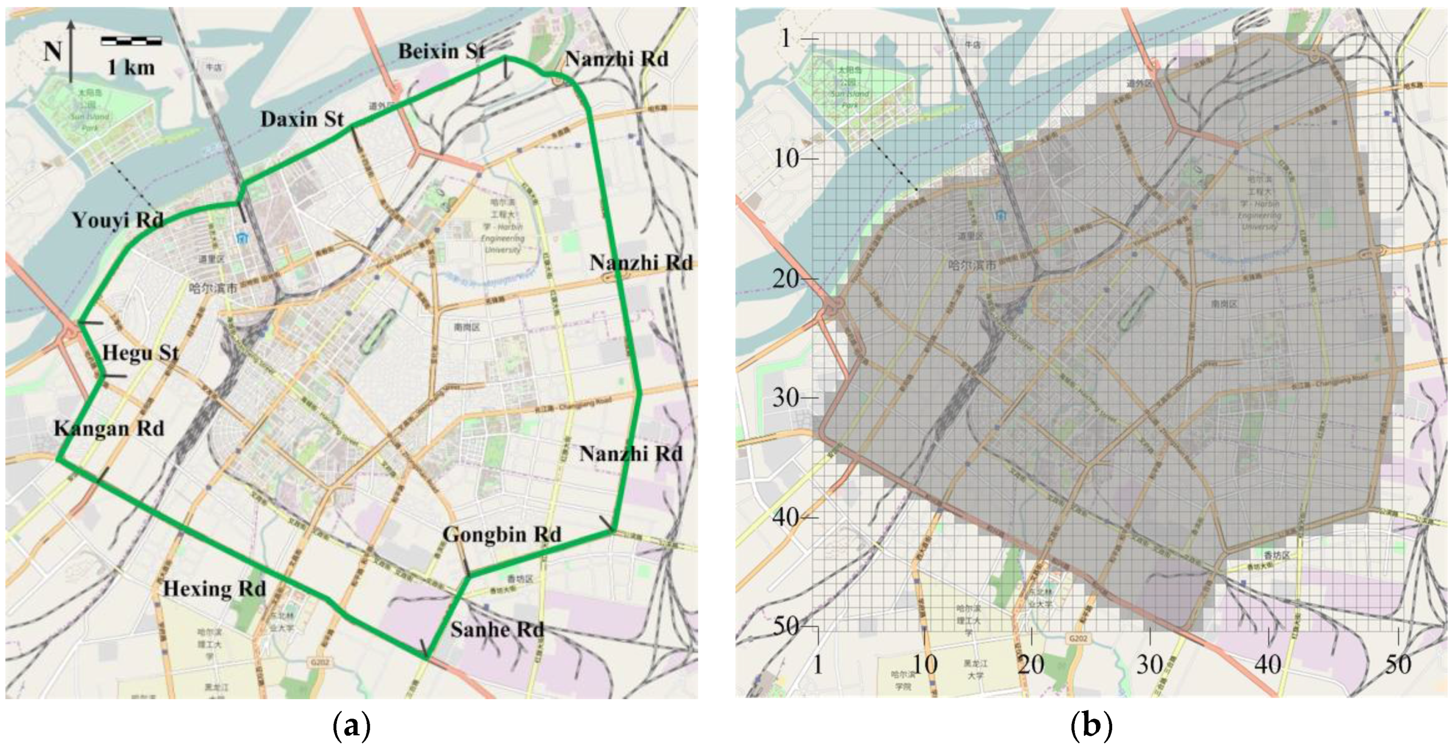
Harbin is the capital of Heilongjiang Province and is located in Northeast China. Harbin was ranked as one of the most seriously congested cities in China in 2015 [24], leading us to choose Harbin as the study city. Additionally, the second-ring-road area, which includes Daxin Street, Beixin Street, and Nanzhi Road, was chosen as the specific study area in this paper (Figure 1a). The Harbin second-ring-road is 30 km long and covers 67.2 km2, which was sufficiently large to research recurrent urban patterns.
This paper examined urban recurrent congestion evolution patterns on a macroscopic level. Thus, the study area was divided into many square grids. Generally, smaller square grids capture more urban congestion details. However, the sampling frequency of Harbin GPS data is 30 s, and the average velocity of a Harbin taxi is about 23 km/h [25]. Therefore, on average, a taxi vehicle travels about 190 m in each sampling interval. As such, if the square grid size is too small, one grid cannot capture a taxi location point, even if the vehicle passed through the grid. Therefore, the gird size in this paper was determined to be 200 m.
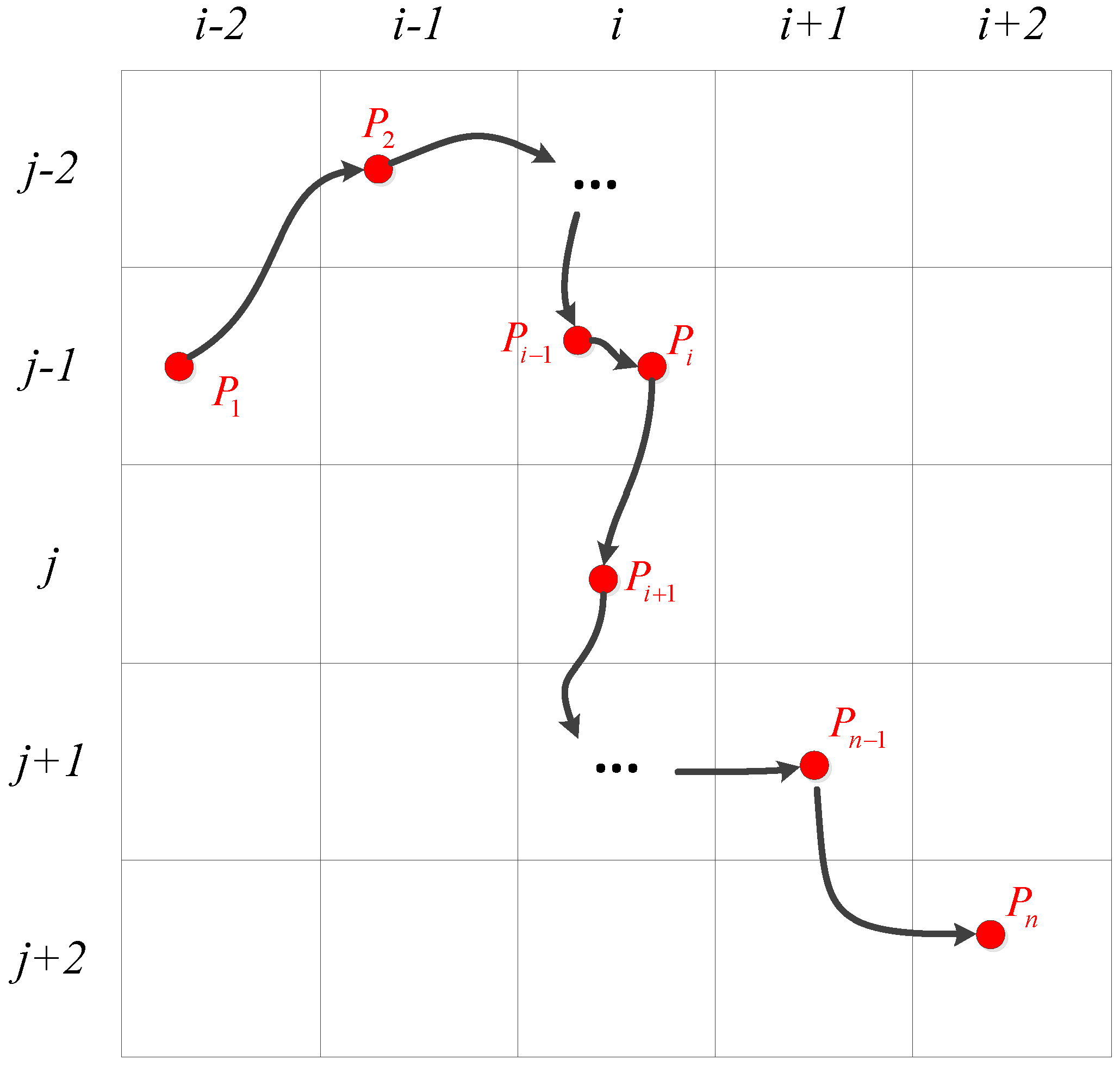
The Harbin second-ring-road area ranges from 45.72 to 45.79 longitude and 126.59 to 126.7 latitude, which is nearly a 10 × 10 km area. We adjusted this range somewhat to 45.712555–45.799049 longitude and 126.582505–26.706473, so that the study area could be divided into integer numbers by 200 m, and the divided grids would still cover the entire second-ring-road area. The divided grids are shown in Figure 1b. There were 2500 grids in total, and 1680 of them were used as the study grids, as shown by the shaded area in Figure 1. The urban area was divided into n × m square grids, and was defined as one specific grid, where and . In Figure 1b, and were both 50. A taxi GPS trajectory was defined as a set of continuous locating points: , and each locating point was defined as: , where , , , , and represent taxi ID, latitude, longitude, timestamp, and instantaneous velocity. Respectively (Table 1). The relationship between the divided grids and a set of GPS trajectories is shown in Figure 2. For the Time Interval , this specific taxi vehicle travels via a set of grids including , , , , , , , and . If only one taxi trajectory exists, each of these 8 grids obtain only one trajectory in , and only grids and obtain one trajectory in , whereas the other 6 grids obtain none.
2.3. Detecting Grid Congestion
Each grid was considered a special traffic detector that can collect traffic flow information. In this study, the number of taxi GPS trajectories (N) and the mean velocity of these GPS trajectories (V) in a specific Time Interval () were obtained for each grid. The mean velocity of the taxi GPS trajectories was calculated as follows:
where is the mean velocity of the th trajectory, and , which is calculated as follow:
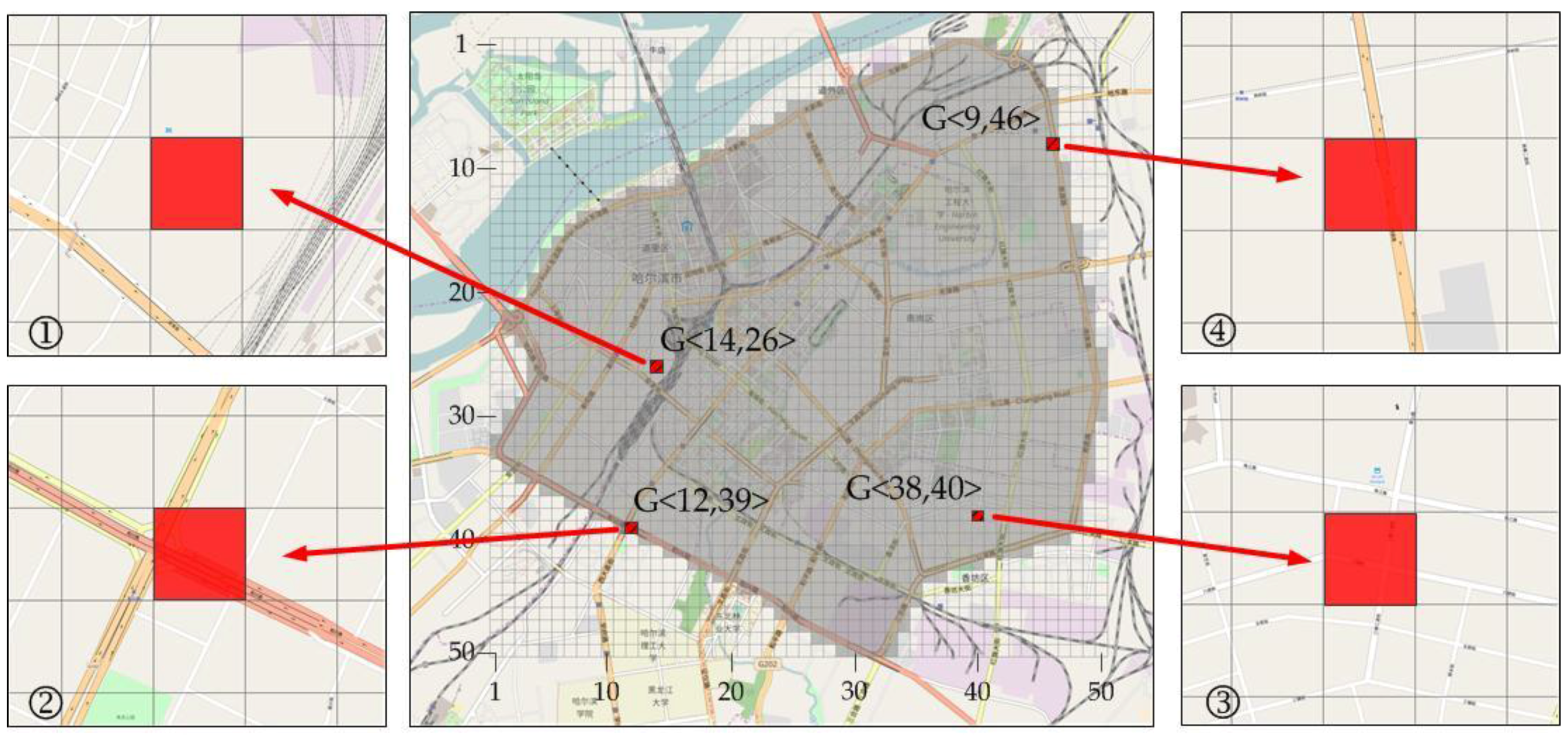
Combined with taxi GPS trajectory and divided grids, three kinds of grid are possible, which are described as follows:
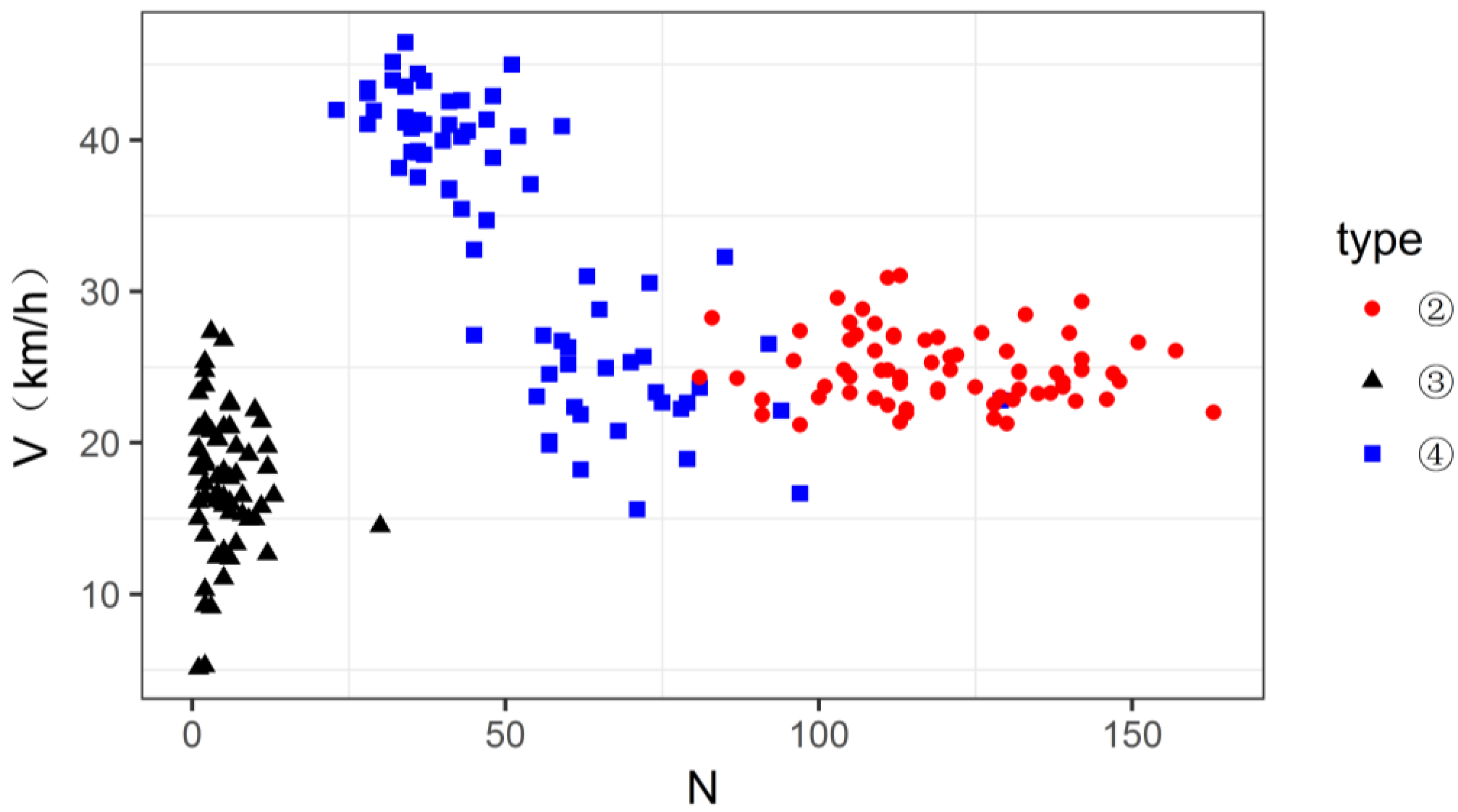
- Type 2: at least one intersection with signal control is included in this kind of grid, such as . Including high-grade road, this kind of grid usually has greater value of and . Due to the signal control, the value of varies minimally, as shown in Figure 4.
- Type 3: at least one intersection with no signal control is included in this kind of grid, such as grid . Including low-grade road, this kind of grid usually obtains a lower value of N. Due to the randomness of the small number of vehicles, V varies considerably, as shown in Figure 4.
- Type 4: no intersection is included in this kind of grid, as per grid . Compared with the other 2 kinds of grids, the variation in and vary considerably, as shown in Figure 4.
Due to the complicated distribution of different grid types, determining a fixed threshold to detect congestion in all kinds of grids was complicated. When congestion typically occurs, a large amount of lower speed vehicles gather in a specific area [5,26], creating an abnormal and pattern As such, grid congestion was detected by calculating the change in taxi trajectory pattern, including and . Therefore, a Grid State () was defined as to reflect the taxi trajectory patterns in a specific grid.
The Euclidean Distance is used to measure the difference between the Grid State in and the Grid State , as follows:
Three times the standard deviation value is usually used for filtering anomalous values in the field of statistics [27]. This was the cut off used in this paper to measure abnormal Grid States (i.e., abnormal taxi trajectory patterns in a specific grid), as follows:
where was calculated as follow:
combined with the lower information:
A specific grid in time interval was identified as being congested if Equations (4) and (6) were both satisfied.
2.4. RC Area Identification
After detecting the congestion of all grids, the RC area (i.e., a set of grids) is discovered in this section.
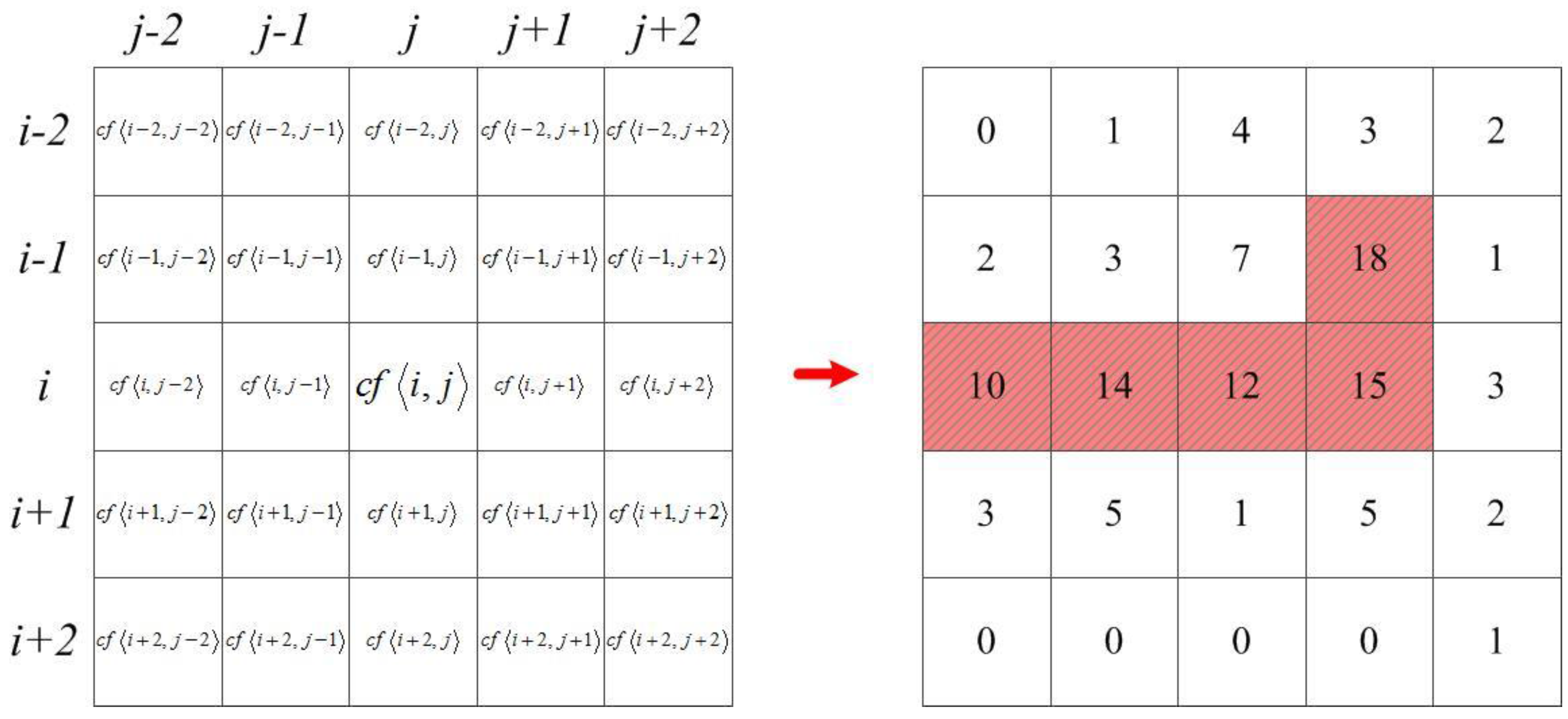
As shown in Figure 5, for a grids area, after identifying grid congestion, the congestion frequency was obtained for a specific period, such as one week or one month. For example, grid was congested during 12 time intervals, so has a congestion frequency () of 12. The spatial adjacent grids that had greater congestion frequency () value were labeled recurrent congestion areas, which were considered during the clustering process [6]. In Figure 5, a 5-grid area with greater congestion frequency was clustered as a recurrent congestion area, consisting of , , , and .
For a grids area, the exact number of clusters (i.e., RC areas) cannot be known in advance, and the shape of the cluster can be random and non-convex. As such, Density-Based Spatial Clustering of Applications with Noise (DBSCAN) was applied to solve this problem. DBSCAN identifies random and non-convex shape clusters and determining the number of clusters in advance is not required [28,29]. We used Liu’s [30] customized DBSCAN algorithm.
2.5. Measuring the RC Evolution Pattern
We first explain the process of one traffic jam. Figure 6 illustrates the five typical congestion states in the congestion process: Congestion Start (CS), Congestion End (CE), Congestion Peak (CP), Congestion Propagation (CPr), and Congestion Dissipation (CD). In Figure 6, the red-shaded grids represent congestion in the corresponding time interval.
The five congestion states are described as follows:
- Congestion Start () represents the beginning of a traffic jam in the specific RC area. represents the start time of a jam, which corresponds to a single time interval. The congested grids in represents the start grids of this jam. In Figure 6, at least one grid is congested in , and none of the 7 grids is congested in the 3 previous time intervals (i.e., , and ), meaning this jam started in .
- Congestion End () is the end of a traffic jam in the specific RC area. is the end time of the jam, which corresponds to a single time interval. In Figure 6, at least one grid is congested in , and none of the 7 grids are congested in the 3 latter time intervals, , and , which means this jam ended in .
- Congestion Peak () is the peak with the maximum number of congested grids in a specific RC area. is the peak time of a jam, which corresponds to at least one time interval. In Figure 6, all the 7 grids are congested in , which means this jam reach peak in . Notably, the particular jam reached a peak in several time intervals, thus the congestion peak contains all states from the first peak to the last.
- Congestion Propagation () is the state between and . represents the propagating time of a jam, which corresponds to several time intervals between and . In Figure 6, this state lasts from to .
- Congestion Dissipation () is the states between and . represents the dissipating time for a jam that corresponds to several time intervals between and . In Figure 6, this state lasts from to .
For a long period such as one week or one month, there are a total of traffic jams occurring in the RC area. The recurrent congestion spatial-temporal evolution pattern details are described in the following section.
2.5.1. RC Temporal Evolution Pattern
Three temporal indicators of the RC are defined as follows:
- RC Start time is calculated as:
- RC End time is calculated as:
- RC time is calculated as:
2.5.2. RC Spatial Evolution Pattern
Two spatial indicators of the RC are as follows:
- RC Start Grid is the set of congested grids in of all traffic jams.
- RC Key Grid is a grid that propagates to the adjacent grids with most frequency. For adjacent grids and , if grid is congested and is not congested in , and then is congested in , it means that traffic jam propagate from to for one time. In Figure 6, the traffic jam propagates from to and in .
3. Experiment and Discussion
3.1. Detecting Grid Congestion
The detecting method was applied for the three types of grids, including (type 2), (type 3) and (type 4). One-week data, from 16–22 November 2015, were used to verify this detecting method. The time interval was set to 10 min, which adequately reflects the change in traffic state in each grid, to ensure each grid obtains enough data to apply the methods [6].
Figure 6 illustrates the ~ distribution of type 2 (i.e., ), type 3 (i.e., ) and type 4 (i.e., ) on 19 December 2015.
Table 2, Table 3 and Table 4 display a sample of the calculated results of the three types of grids on 19 December 2015.
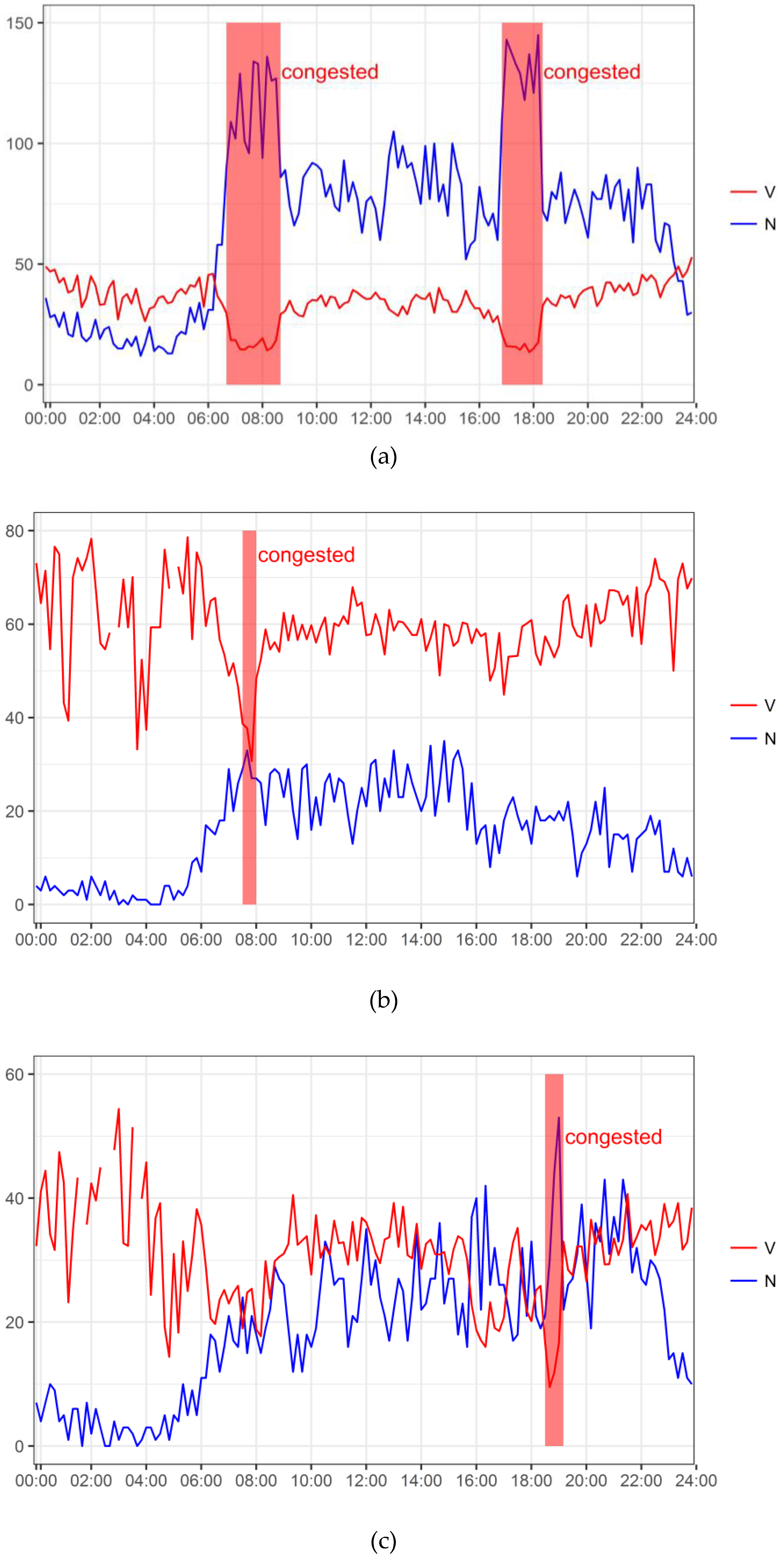
In Table 2, Equations (4) and (6) were both satisfied from 4:50 to 6:20 p.m., for a total of nine time intervals, which means grid was congested during these intervals. As shown in Figure 7a, the and distrbutions appear to be abnoraml in these time intervals, with greater and lower . The and distributions present regularly, as shown in Figure 8a. The congestion of grid occurred during the moring and evening peak hours of each day from 16–22 December 2015, demonstrating periodicity.
In Table 3, Equation (4) and (6) were both satisfied from 07:40 to 08:10 a.m., for a total if three time intervals, which means grid ws congested during these intervals. As shown in Figure 7b, the and distrbutions appear to be abnormal in these time intervals, with greater and lower . The and distrbutions of grid present regularly, as shown in Figure 8b. The congestion of grid occurred at the peak morning hours of each day for 16–22 December 2015, demonstrating periodicity.
In Table 4, Equations (4) and (6) were both satisfied from 6:50 to 7:20 p.m., for a total of three time intervals, which means grid was congested during these intervals. As shown in Figure 7c, the and distributions appear to be abnormal in these time intervals, with greater and lower . The and distributions of grid show regularity, as displayed in Figure 8c. The congestion of grid occurred at the evening peak hours of each day (day for 16–22 December 2015, demonstrating periodicity.
3.2. Measuring the RC Evolution Pattern
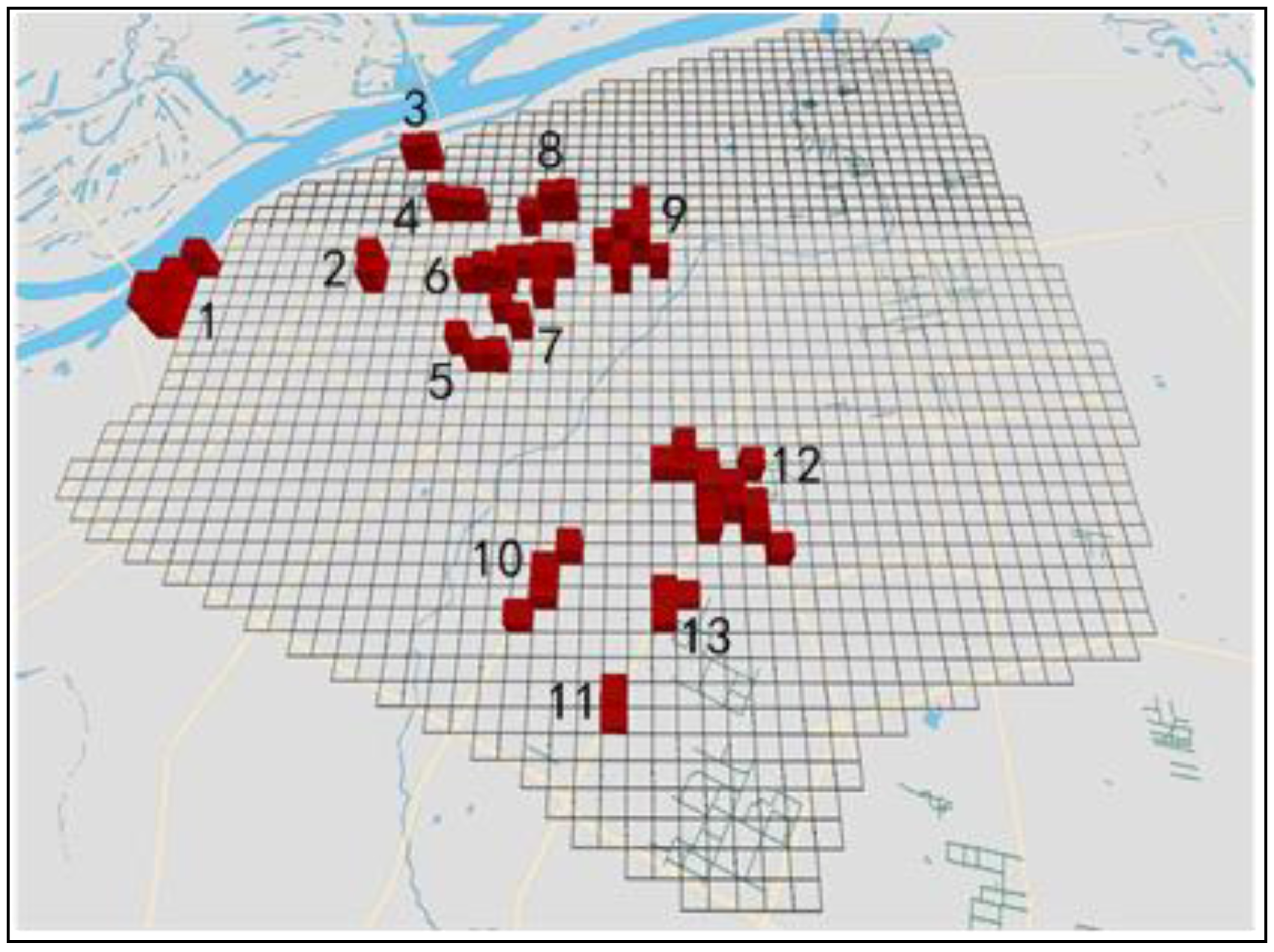
The data from the 25 days were applied in the customized DBSCAN algorithm [30]. A total 13 recurrent congestion areas were discovered in Harbin second-ring road area at morning peak hours, which are shown in Figure 9. The threshold of congestion frequency was set to 375, which means that all 13 recurrent congestion grids were detected to be congested in more than 15 time intervals for each day on average. That is to say, the values of all the recurrent congestion were more than 150 min. The 13 RC areas included 62 grids, 4.8 grids on average.
The details of spatial evolution pattern of the recurrent congestion occur in the 13 RC areas are illustrated in Table 5.
- Some remarkable characteristics of the RC spatial evolution patterns were observed during the winter in Harbin at morning peak hours. Firstly, the RC spatial distribution is extremely uneven. In the second-rind road area of Harbin, the 13 RC areas are concentrated in two main regions, as shown in Figure 10. The first area is a two-kilometer radius circular region, centered on Harbin Train Station. This region is in the northwest part of the urban Harbin area, containing eight RC areas. The second area is also a two-kilometer radius circular region, centered on the Heilongjiang Provincial Government Office Building. This region is in the southern part of the Harbin urban area, containing 4 RC areas. Secondly, the RC areas are very different from each other. The RC range varied considerably. For example, Cluster 12 included 13 grids, with a value almost eight times that of those found in Clusters 2, 3, 7, and 11. The Start Grid (or Key Grid) types are different. For example, the Start Grid in Cluster 12 () is type 2, whereas it is type 3 in Cluster 7 ().
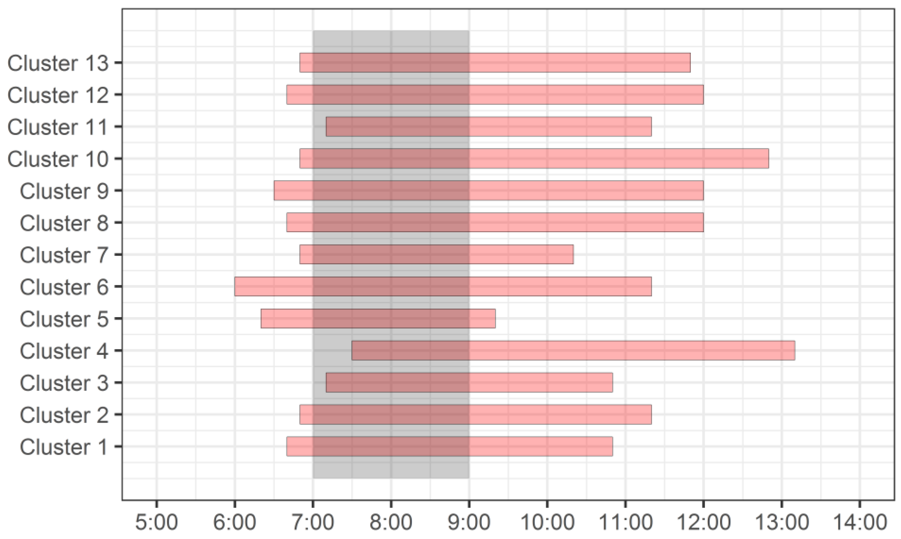
The temporal evolution pattern of the recurrent congestion occur in the 13 RC areas are illustrated in Figure 11.
- Some remarkable characteristics of the RC temporal evolution patterns were observed during the winter in Harbin at peak morning hours. The start time of most RC is earlier than morning peak hours. Generally speaking, the urban morning peak hours were from 7:00 to 9:00 a.m., with 77% (N = 10) of the RC appearing earlier than 7:00 a.m. On average, the RC start time was 6:45 a.m. The earliest RC start time was observed in Cluster 6 at 6:00 a.m. additionally, the end times for all RC were later than the morning peak hours. All the RC disappeared after 9:00 a.m., and 92% (N = 12) disappeared after 10:00 a.m. The RC that occurred in Clusters 4 and 10 did not end until afternoon. We also noted that the duration of all RC was longer than the morning peak hours. All the RC lasted for more than two hours. The average congestion time for all RC was 4.7 h.
3.3. Discussion
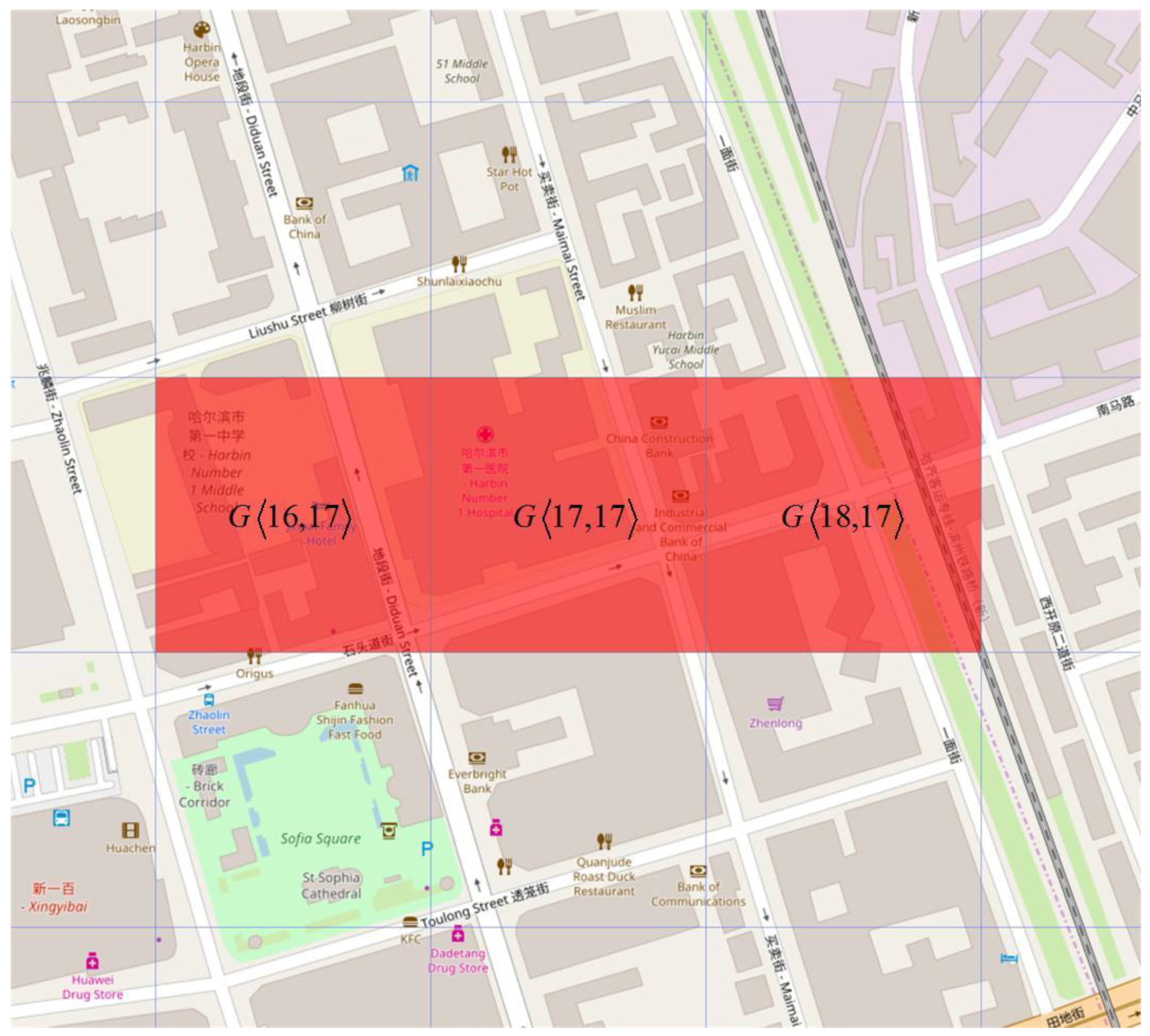
One of the aims of this paper was to determine how understanding the RC evolution patterns would help operators and traffic planners to analyze causes and create alleviating strategies. Due to the complicated situation of each RC area, the causal factors and alleviating strategies for all 13 RC areas are different. Therefore, a typical RC area, Cluster 4, was selected as an example.
As shown in Figure 12, Cluster 4 has three grids, , , and . Shitoudao, Diduan, Maimai, and Yimian Streets are in these three grids. The RC that occurs in this area usually starts at 7:30 a.m. The start grid is . The congestion usually propagates from to and along with Shitoudao Street. The grid that most frequently propagates to the adjacent grids (i.e., the RC Key Grid) was .
3.3.1. RC Cause Analysis
Harbin No. 1 Middle School and Harbin No. 1 Hospital are in this RC area, which place high demands on the roadway infrastructure. The school and hospital both open at 8:00 a.m., and heavy traffic travels along with Shitoudao Street from east to west, where drivers must turn right to reach the entrance of the school and hospital. The entrances are in on Diduan Street, which is a north–south one-way street. Shitoudao Street is the only way to reach the entrances, which has only one east–west lane. Therefore, the RC usually first appears in when heavy traffic exceeds the road capacity. Then the RC spreads to upstream areas, such as and ).
3.3.2. RC Alleviating Strategies
Due to the lack of parking spaces for Harbin No.1 Middle School and Harbin No. 1 Hospital, many roadside temporary parking spaces exist along Shitoudao and Diduan Streets. Parking lots should be constructed for Harbin No. 1 Middle School and Harbin No. 1 Hospital to meet the parking demands. In addition, administration and supervision should be strengthened to reduce the temporary roadside parking. Also, Shitoudao Street (from east to west) should be rebuilt to increase traffic capacity.
4. Conclusions
Taxi GPS trajectories are valuable resources that can be used to measure urban recurrent congestion and evolution patterns. Based on taxi GPS trajectories, we proposed a novel stepwise method to measure the recurrent urban congestion evolution patterns. We also completed a case study in the urban Harbin area, using real GPS data and digital maps rather than simulation data. In understanding the RC evolution patterns, the city traffic manager can visualize recurrent urban congestion at the macroscopic level. The main contributions of this paper can be summarized as follows:
- (1)
- The main method proposed is based on taxi trajectory data, which has obvious advantages including extensive coverage and lower cost in comparison with the data collected from traditional traffic detectors, such as loops, microwaves, and video detectors.
- (2)
- We created the grid congestion detection method using multivariate trajectory pattern analysis, including the number of taxi trajectories and their average velocity. Then, a rule was used to detect abnormal patterns in the grid. Combined with the lower average velocity information, a specific grid is identified as being congested.
- (3)
- An integrated stepwise method is proposed to measure urban RC evolution patterns at the macroscopic level, including detecting grid congestion, determining RC areas, and measuring the RC evolution patterns. The method provides a new solution for Intelligent Transportation System application.
- (4)
- Based on the proposed methods, a case study was completed in Harbin, China with real GPS data and a digital map, rather than simulation data, to evaluate the stepwise method. A total of 13 RC areas were detected that occur in the Harbin second ring road area in winter during peak morning hours. In addition, some remarkable spatial-temporal evolution pattern characteristics of RC were revealed in this paper.
Further studies may expand the data source to other GPS-equipped vehicles. In addition, by using the results of the RC evolution pattern, congestion prediction method could be proposed.
Acknowledgments
This research is supported by the National Natural Science Foundation of China (General Program 51478151; General Program 51578199; Major Program 71390522). This work was performed at the Key Laboratory of Advanced Materials & Intelligent Control Technology on Transportation Safety, Ministry of Communications, China.
Author Contributions
An Shi designed the framework of the paper. The Introduction, Methods and Results and Conclusions were developed jointly by An Shi, Yang Haiqiang and Wang Jian. The Experiment and Discussion was carried out by Yang Haiqiang.
Conflicts of Interest
The authors declare no conflict of interest.
References
- Moreira-Matias, L.; Alesiani, F. Drift3Flow: Freeway-Incident Prediction Using Real-Time Learning. In Proceedings of the IEEE International Conference on Intelligent Transportation Systems, Las Palmas, Spain, 15–18 September 2015; pp. 566–571. [Google Scholar]
- Chung, Y. Identification of Critical Factors for Non-Recurrent Congestion Induced by Urban Freeway Crashes and Its Mitigating Strategies. Sustainability 2017, 9, 2331. [Google Scholar] [CrossRef]
- Moreira-Matias, L.; Cerqueira, V. CJAMmer—Traffic JAM Cause Prediction using Boosted Trees. In Proceedings of the IEEE International Conference on Intelligent Transportation Systems, Rio de Janeiro, Brazil, 1–4 November 2016; pp. 743–748. [Google Scholar]
- Gurupackiam, S.; Jones, S.L., Jr. Empirical Study of Accepted Gap and Lane Change Duration within Arterial Traffic under Recurrent and Non-Recurrent Congestion. Int. J. Traffic Transp. Eng. 2012, 2, 306–322. [Google Scholar] [CrossRef]
- Schimbinschi, F.; Moreira-Matias, L.; Nguyen, V.X.; Bailey, J. Topology-regularized universal vector autoregression for traffic forecasting in large urban areas. Expert Syst. Appl. 2017, 82, 301–316. [Google Scholar] [CrossRef]
- An, S.; Yang, H.; Wang, J.; Cui, N.; Cui, J. Mining urban recurrent congestion evolution patterns from GPS-equipped vehicle mobility data. Inf. Sci. 2016, 373, 515–526. [Google Scholar] [CrossRef]
- Li, R.; Pereira, F.C.; Benakiva, M.E. Competing risks mixture model for traffic incident duration prediction. Accid. Anal. Prev. 2015, 75, 192–201. [Google Scholar] [CrossRef] [PubMed]
- Cui, J.X.; Liu, F.; Janssens, D.; An, S.; Wets, G.; Coolsc, M. Detecting urban road network accessibility problems using taxi GPS data. J. Transp. Geogr. 2016, 51, 147–157. [Google Scholar] [CrossRef]
- Hwang, R.H.; Hsueh, Y.L.; Chen, Y.T. An effective taxi recommender system based on a spatio-temporal factor analysis model. Inf. Sci. 2015, 314, 28–40. [Google Scholar] [CrossRef]
- Woodard, D.; Nogin, G.; Koch, P.; Racz, D.; Goldszmidt, M.; Horvitz, E. Predicting travel time reliability using mobile phone GPS data. Transp. Res. Part C Emerg. Technol. 2017, 75, 30–44. [Google Scholar] [CrossRef]
- Lu, S.F.; Mai, Y.H.; Liu, X.M. The Analysis of Characterization of Urban Traffic Congestion Based on Mixed Speed Distribution of Taxi GPS Data. Appl. Mech. Mater. 2013, 241–244, 2076–2081. [Google Scholar] [CrossRef]
- Cui, J.X.; Liu, F.; Hu, J.; Janssens, D.; Wets, G.; Cools, M. Identifying mismatch between urban travel demand and transport network services using GPS data: A case study in the fast growing Chinese city of Harbin. Neurocomputing 2016, 181, 4–18. [Google Scholar] [CrossRef]
- Daganzo, C.F. The cell transmission model: A dynamic representation of highway traffic consistent with the hydrodynamic theory. Transp. Res. Part B Methodol. 1994, 28, 269–287. [Google Scholar] [CrossRef]
- Chandler, R.E.; Herman, R.; Montroll, E.W. Traffic dynamics: Studies in car following. Oper. Res. 1958, 6, 165–184. [Google Scholar] [CrossRef]
- Zhang, A.; Gao, Z. CTM-based Propagation of Non-recurrent Congestion and Location of Variable Message Sign. In Proceedings of the Fifth International Joint Conference on Computational Sciences and Optimization, Harbin, China, 23–26 June 2012; pp. 462–465. [Google Scholar]
- Chu, C.; Xie, N.; Chen, X.; Wu, Y.; Sun, X. Temporal-Spatial Analysis of Traffic Congestion Based on Modified CTM. Math. Probl. Eng. 2015, 2015, 1–11. [Google Scholar] [CrossRef]
- Yang, Y.; Hu, Z.A.; Yan, Y.S. Incident-based traffic congestion propagation mechanism with improved CTM model. Beijing Gongye Daxue Xuebao 2015, 41, 1061–1066. [Google Scholar]
- Chen, D.; Laval, J.; Zheng, Z.; Ahn, S. A behavioral car-following model that captures traffic oscillations. Transp. Res. Part B Methodol. 2012, 46, 744–761. [Google Scholar] [CrossRef] [Green Version]
- Zhu, F.; Hong, K.L.; Lin, H.Z. Delay and emissions modelling for signalised intersections. Transp. B Transp. Dyn. 2013, 1, 111–135. [Google Scholar] [CrossRef]
- Papathanasopoulou, V.; Antoniou, C. Towards data-driven car-following models. Transp. Res. Part C Emerg. Technol. 2015, 55, 496–509. [Google Scholar] [CrossRef]
- Hofleitner, A.; Herring, R.; Abbeel, P.; Bayen, A. Learning the Dynamics of Arterial Traffic from Probe Data Using a Dynamic Bayesian Network. IEEE Trans. Intell. Transp. Syst. 2012, 13, 1679–1693. [Google Scholar] [CrossRef]
- Castro, P.S.; Zhang, D.; Chen, C.; Li, S.; Pan, G. From taxi GPS traces to social and community dynamics: A survey. ACM Comput. Surv. 2013, 46, 17. [Google Scholar] [CrossRef]
- Zheng, H.; Wang, Y.; Cang, Y. Research of the four seasons division of Harbin. Heilongjian Clim. 2001, 3, 32–33. [Google Scholar]
- The Congestion Ranking of Main Cities in China. Available online: report.amap.com/congestion.do (accessed on 10 January 2016).
- Tang, J.; Liu, F.; Wang, Y.; Wang, H. Uncovering urban human mobility from large scale taxi GPS data. Phys. Stat. Mech. Appl. 2015, 438, 140–153. [Google Scholar] [CrossRef]
- Zheng, K.; Zheng, Y.; Yuan, N.J.; Shang, S.; Zhou, X. Online Discovery of Gathering Patterns over Trajectories. IEEE Trans. Knowl. Data Eng. 2013, 8, 242–253. [Google Scholar] [CrossRef]
- Lehmann, R. 3σ-Rule for Outlier Detection from the Viewpoint of Geodetic Adjustment. J. Surv. Eng. 2014, 139, 157–165. [Google Scholar] [CrossRef]
- Huang, F.; Zhu, Q.; Zhou, J.; Tao, J.; Zhou, X.; Jin, D.; Tan, X.; Wang, L. Research on the Parallelization of the DBSCAN Clustering Algorithm for Spatial Data Mining Based on the Spark Platform. Remote Sens. 2017, 9, 1301. [Google Scholar] [CrossRef]
- Mao, Y.; Zhong, H.; Qi, H.; Ping, P.; Li, X. An Adaptive Trajectory Clustering Method Based on Grid and Density in Mobile Pattern Analysis. Sensors 2017, 17, 2013. [Google Scholar] [CrossRef] [PubMed]
- Liu, Y.; Yan, X.; Wang, Y.; Yang, Z.; Wu, J. Grid Mapping for Spatial Pattern Analyses of Recurrent Urban Traffic Congestion Based on Taxi GPS Sensing Data. Sustainability 2017, 9, 533. [Google Scholar] [CrossRef]
Figure 1.
Illustration of the study area: (a) The second-ring-road in Harbin, China, and (b) The study area divided into grids.
Figure 1.
Illustration of the study area: (a) The second-ring-road in Harbin, China, and (b) The study area divided into grids.

Figure 2.
Illustration of relationship between grids and GPS trajectory.

Figure 3.
Illustration of three kinds of grid.

Figure 4.
The - scatterplot of different grid types (the data are collected on 21 December 2015, and the time interval is 10 min of nature time.).
Figure 4.
The - scatterplot of different grid types (the data are collected on 21 December 2015, and the time interval is 10 min of nature time.).

Figure 5.
The example of congestion frequency of grids.

Figure 6.
A typical congestion process occurring in a seven-grid area.
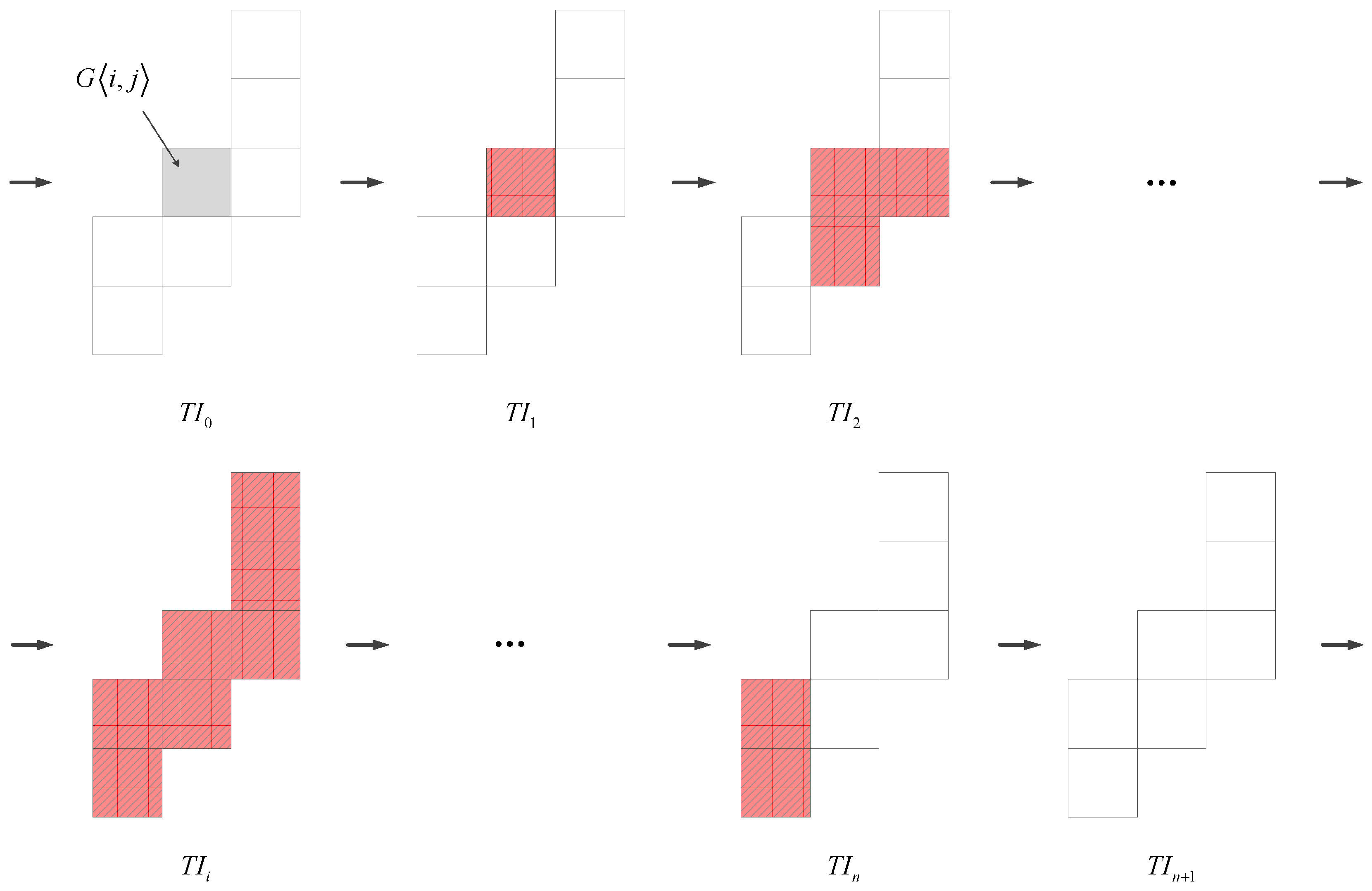
Figure 7.
The - distribution of three types of grids on 19 December 2015: (a) The - distribution of type 2 grid (i.e., ); (b) The - distribution of type 4 grid (i.e., ); (c) The - distribution of type 4 grid (i.e., ).
Figure 7.
The - distribution of three types of grids on 19 December 2015: (a) The - distribution of type 2 grid (i.e., ); (b) The - distribution of type 4 grid (i.e., ); (c) The - distribution of type 4 grid (i.e., ).

Figure 8.
The and distributions in one week from 16–22 December 2015 for three types of grid: (a) Grid ; (b) Grid ; (c) Grid .
Figure 8.
The and distributions in one week from 16–22 December 2015 for three types of grid: (a) Grid ; (b) Grid ; (c) Grid .
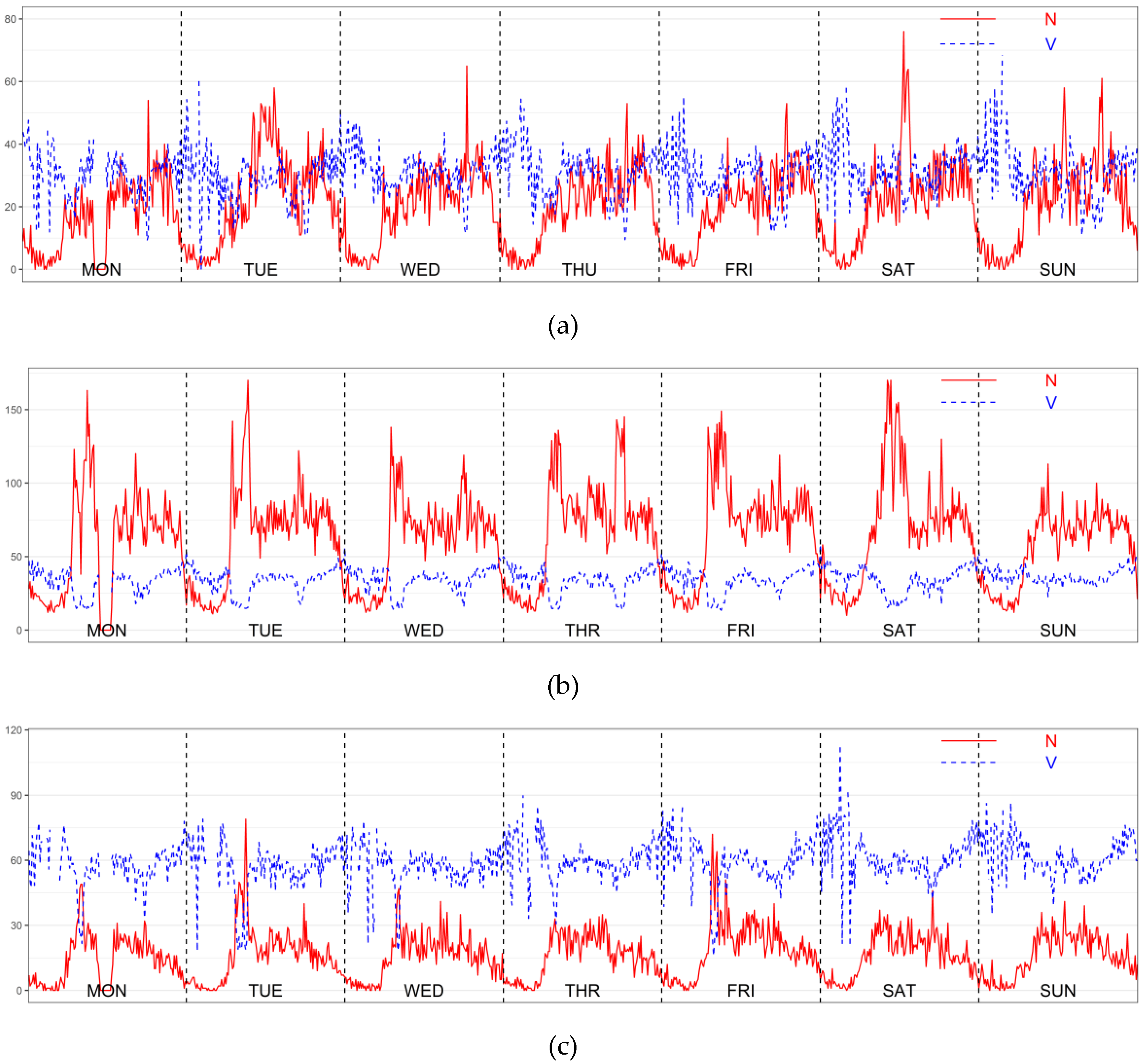
Figure 9.
The 13 recurrent congestion areas in the Harbin second-ring road area.

Figure 10.
The spatial distribution of the recurrent congestion (RC) areas.
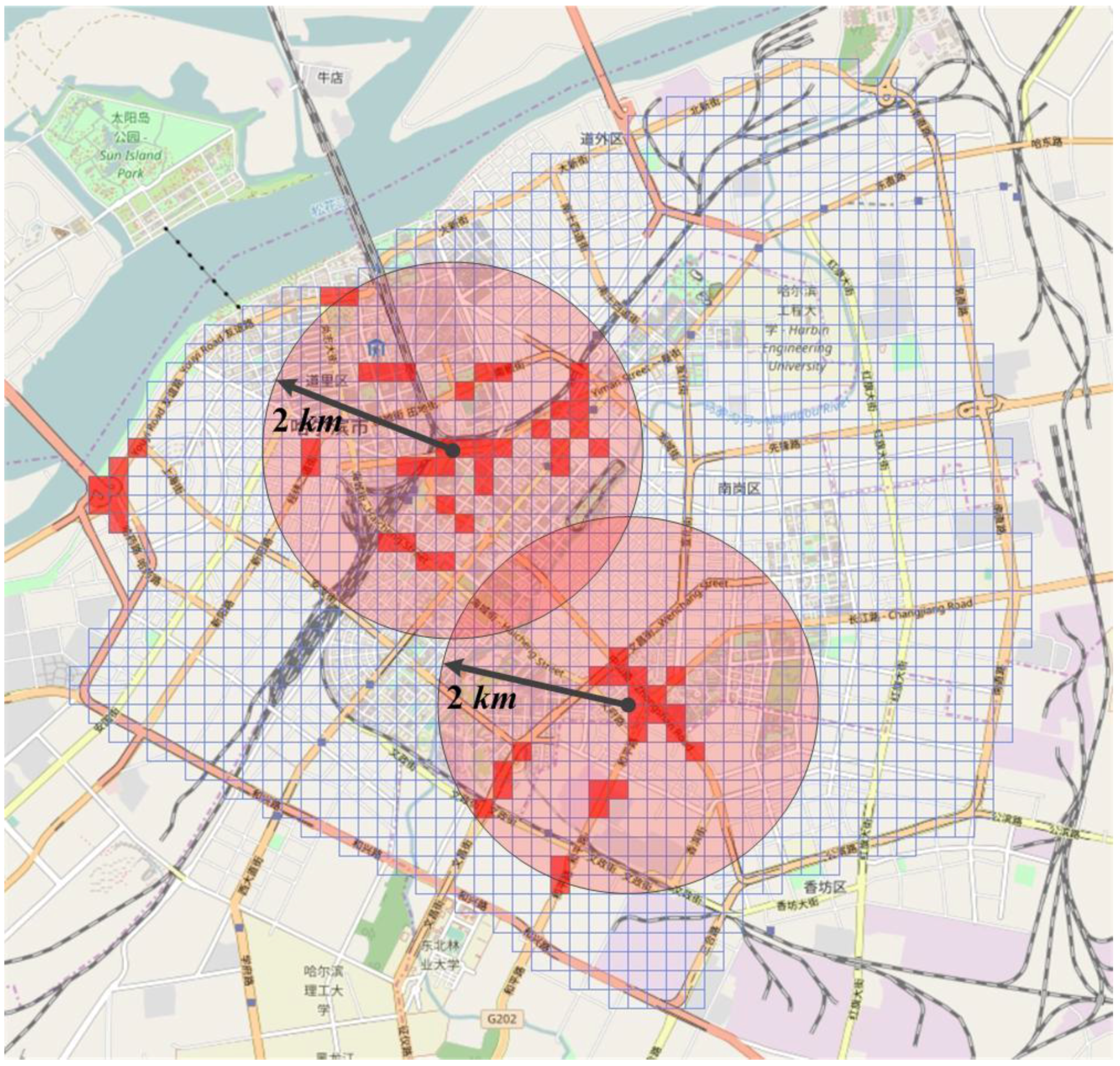
Figure 11.
The temporal evolution pattern of the 13 recurrent congestion areas.

Figure 12.
The three grids of Cluster 4.

Table 1.
A typical global positioning system (GPS) taxi records.
| Taxi ID | Latitude | Longitude | Timestamp | Instantaneous Velocity () |
|---|---|---|---|---|
| 0100322231 | 45.77463 | 126.63945 | 23-02-2015 6:58:51 | 19.6 |
| 0100322231 | 45.77463 | 126.63693 | 23-02-2015 6:59:21 | 22.1 |
| 0100322231 | 45.77461 | 126.63701 | 23-02-2015 6:59:51 | 21.9 |
| 0100322231 | 45.77462 | 126.63711 | 23-02-2015 7:00:21 | 12.5 |
| 0100322231 | 45.77462 | 126.6371 | 23-02-2015 7:00:51 | 0 |
Table 2.
Sample of the calculation results for the type 2 grid.
| TI | GS<N,V> | GSavg[ ] | Left of Equation (4) | Right of Equation (4) | Satisfy Equation (4) | Satisfy Equation (6) | Congested |
|---|---|---|---|---|---|---|---|
| … | … | … | … | … | … | … | … |
| 16:10–16:20 | <70,27.6> | <61.8,33.7> | 22.7 | 30.7 | FALSE | TRUE | FALSE |
| 16:20–16:30 | <66,30.9> | <61.8,33.6> | 10 | 15 | FALSE | TRUE | FALSE |
| 16:30–16:40 | <71,25.9> | <61.9,33.6> | 24.9 | 35.7 | FALSE | TRUE | FALSE |
| 16:40–16:50 | <60,28.5> | <61.9,33.5> | 11.5 | 16.1 | FALSE | TRUE | FALSE |
| 16:50–17:00 | <110,21> | <62.4,33.4> | 180.1 | 147.7 | TRUE | TRUE | TRUE |
| 17:00–17:10 | <143,16.1> | <63.1,33.2> | 300.5 | 245 | TRUE | TRUE | TRUE |
| 17:10–17:20 | <138,15.9> | <63.9,33.1> | 278.7 | 228.3 | TRUE | TRUE | TRUE |
| 17:20–17:30 | <133,15.8> | <64.5,32.9> | 241.4 | 211.8 | TRUE | TRUE | TRUE |
| 17:30–17:40 | <129,14.5> | <65.1,32.7> | 237.4 | 199.3 | TRUE | TRUE | TRUE |
| 17:40–17:50 | <118,17.1> | <65.6,32.6> | 211.6 | 163.9 | TRUE | TRUE | TRUE |
| 17:50–18:00 | <137,13.3> | <66.3,32.4> | 255.4 | 219.6 | TRUE | TRUE | TRUE |
| 18:00–18:10 | <121,15.1> | <66.8,32.2> | 202.6 | 170.6 | TRUE | TRUE | TRUE |
| 18:10–18:20 | <145,17.7> | <67.5,32.1> | 344.7 | 236.5 | TRUE | TRUE | TRUE |
| 18:20–18:30 | <72,32.8> | <67.5,32.1> | 29.1 | 13.6 | TURE | FALSE | FALSE |
| 18:30–18:40 | <68,35.9> | <67.5,32.1> | 20.4 | 11.3 | TRUE | FALSE | FALSE |
| 18:40–18:50 | <80,33.7> | <67.6,32.2> | 32.9 | 37.3 | FALSE | FALSE | FALSE |
| … | … | … | … | … | … | … | … |
Table 3.
Sample of the calculation results of the type 3 grid.
| TI | GS<N,V> | GSavg[ ] | Left of Equation (4) | Right of Equation (4) | Satisfy Equation (4) | Satisfy Equation (6) | Congested |
|---|---|---|---|---|---|---|---|
| … | … | … | … | … | … | … | … |
| 07:10–07:20 | <29,49> | <5.2,64> | 69.3 | 84.5 | FALSE | TRUE | FALSE |
| 07:20–07:30 | <20,51.7> | <5.5,63.7> | 49.6 | 56.5 | FALSE | TRUE | FALSE |
| 07:30–07:40 | <26,46.6> | <6,63.3> | 65.1 | 78.3 | FALSE | TRUE | FALSE |
| 07:40–07:50 | <29,38.7> | <6.5,62.8> | 118.6 | 99 | TRUE | TRUE | TRUE |
| 07:50–08:00 | <33,37.7> | <7,62.3> | 127.4 | 107.1 | TRUE | TRUE | TRUE |
| 08:00–08:10 | <27,30.7> | <7.5,61.6> | 140.4 | 109.7 | TRUE | TRUE | TRUE |
| 08:10–08:20 | <27,48.3> | <7.9,61.3> | 51.4 | 69.5 | FALSE | TRUE | FALSE |
| 08:20–08:30 | <26,52.5> | <8.2,61.1> | 44.2 | 59.3 | FALSE | TRUE | FALSE |
| … | … | … | … | … | … | … | … |
Table 4.
Sample of the calculation results for the type 4 grid.
| TI | GS<N,V> | GSavg[ ] | Left of Equation (4) | Right of Equation (4) | Satisfy Equation (4) | Satisfy Equation (6) | Congested |
|---|---|---|---|---|---|---|---|
| … | … | … | … | … | … | … | … |
| 18:00–18:10 | <21,21.8> | <16.7,31.2> | 25.5 | 31.1 | FALSE | TRUE | FALSE |
| 18:10–18:20 | <33,20.1> | <16.8,31.1> | 37.1 | 58.6 | FALSE | TRUE | FALSE |
| 18:20–18:30 | <21,25.1> | <16.9,31> | 18.1 | 21.6 | FALSE | TRUE | FALSE |
| 18:30–18:40 | <19,25.9> | <16.9,31> | 16.6 | 16.7 | FALSE | TRUE | FALSE |
| 18:40–18:50 | <21,16.7> | <16.9,30.9> | 31.6 | 44.2 | FALSE | TRUE | FALSE |
| 18:50–19:00 | <30,9.5> | <17,30.7> | 132.4 | 74.5 | TRUE | TRUE | TRUE |
| 19:00–19:10 | <44,11.9> | <17.3,30.5> | 174.9 | 97.8 | TRUE | TRUE | TRUE |
| 19:10–19:20 | <53,16.6> | <17.6,30.4> | 205.7 | 114 | TRUE | TRUE | TRUE |
| 19:20–19:30 | <22,33> | <17.6,30.4> | 24.4 | 15.3 | TRUE | FALSE | FALSE |
| 19:30–19:40 | <26,28.4> | <17.7,30.4> | 22 | 25.6 | FALSE | TRUE | FALSE |
| 19:40–19:50 | <27,27.5> | <17.8,30.4> | 26.4 | 29 | FALSE | TRUE | FALSE |
| 19:50–20:00 | <31,32.2> | <17.9,30.4> | 30.6 | 39.8 | FALSE | FALSE | FALSE |
| … | … | … | … | … | … | … | … |
Table 5.
The details of spatial evolution pattern of all recurrent congestion.
| Cluster ID | Gird Number | RC Start Grid | RC Key Grid | Functional Zone |
|---|---|---|---|---|
| 1 | 7 | G<2,24> G<2,24> | G<3,23> | Urban main road |
| 2 | 2 | G<13,21> | G<13,21> | Residence Zone |
| 3 | 2 | G<14,13> | G<14,13> | Educational Zone |
| 4 | 3 | G<16,17> | G<16,17> | Public Service Zone |
| 5 | 3 | G<19,27> | G<19,27> | Residence Zone |
| 6 | 9 | G<19,22> | G<19,22> | Public Service Zone |
| 7 | 2 | G<20,24> | G<20,24> | Urban main road |
| 8 | 3 | G<23,17> | G<23,17> | Public Service Zone |
| 9 | 9 | G<26,19> | G<27,20> | Mixed Functional Zone |
| 10 | 4 | G<24,38> | G<24,38> | Urban main road |
| 11 | 2 | G<26,43> | G<26,43> | Educational Zone |
| 12 | 13 | G<30,35> | G<30,34> | Urban main road |
| 13 | 3 | G<28,40> | G<28,40> | Residence Zone |
© 2018 by the authors. Licensee MDPI, Basel, Switzerland. This article is an open access article distributed under the terms and conditions of the Creative Commons Attribution (CC BY) license (http://creativecommons.org/licenses/by/4.0/).
Share and Cite
MDPI and ACS Style
An, S.; Yang, H.; Wang, J. Revealing Recurrent Urban Congestion Evolution Patterns with Taxi Trajectories. ISPRS Int. J. Geo-Inf. 2018, 7, 128. https://doi.org/10.3390/ijgi7040128
AMA Style
An S, Yang H, Wang J. Revealing Recurrent Urban Congestion Evolution Patterns with Taxi Trajectories. ISPRS International Journal of Geo-Information. 2018; 7(4):128. https://doi.org/10.3390/ijgi7040128
Chicago/Turabian StyleAn, Shi, Haiqiang Yang, and Jian Wang. 2018. "Revealing Recurrent Urban Congestion Evolution Patterns with Taxi Trajectories" ISPRS International Journal of Geo-Information 7, no. 4: 128. https://doi.org/10.3390/ijgi7040128
Note that from the first issue of 2016, this journal uses article numbers instead of page numbers. See further details here.