1. Introduction
In the 75 years since the introduction of ANNs basically in Neuroscience [
1], their use has expanded to numerous fields, including Economics, Mathematics, Meteorology, Clinical Medicine, Environmental Area etc. Specifically in recent years, ANNs have found a number of applications in the area of recognition and classification [
2], water quality [
3,
4], meteorology [
5], politics [
6], medical diagnostics [
7] etc. Therefore, it appears that the ANNs are used in applications for classification, clustering, association, regression, modeling and forecasting.
Moreover, ANNs have also been introduced to solve various problems in the scientific field of Geodesy. They have been used in the regional mapping of the Geoid [
8], sea level prediction [
9], coordinate transformation [
10], Coordinated Universal Time (UTC) correction [
11,
12] etc.
In brief, an ANN is an artificial intelligence technique that mimics the human brain’s biological neural network. It is defined as a system of simple processing elements called “artificial neurons”, which are typically organized in layers, so that each ANN includes: an input layer, hidden layers (which can have neurons linked in different ways to the other hidden layers or to the output layer) and an output layer. The main feature of ANNs is their inherent capacity to learn, a key component of their intelligence. Learning is achieved through training, a repetitive process of gradual adaptation of the network’s parameters to the values required to solve a problem [
13,
14,
15,
16,
17,
18,
19].
Before analyzing the proposed forecasting methodology it is essential to mention, the worldwide used forecasting techniques. The techniques, which are used in order to produce a forecast, can be separated in two main categories: the Judgmental Forecasting Techniques and the Statistical Forecasting Techniques [
20]. However, there is another alternative way of separate these techniques in: the Judgmental ones, the Extrapolative, the Econometric and finally the Non-Linear Computer-intensive ones.
Finally, they can also be distinguished, according to the method which is used in order to produce the forecast, in the following categories: Quantitative forecasting (as Timeseries methods, Causal Relationship or Explanatory methods and Artificial Intelligence methods), Qualitative or Judgmental forecasting (as Individual methods and Committee methods) and Technological forecasting (as Exploratory methods and Normative methods). Also the above mentioned techniques can further split in their corresponding subcategories [
21], e.g., the Timeseries methods consist of exponential smoothing method, Kalman Filters [
22,
23], Box Jenkins ARIMA methods, multiple regression methods, and so on.
After the necessary bibliographic research, it was found that in the scientific field of Geodesy the main interest of the Geodesists is focused on monitoring of a phenomenon rather than on its forecasting. Thus, it was emerged that there is no methodology, which could be used in order to forecast the change of a point position on an artificial structure or on the earth surface. The majority of the techniques or models are focused on the monitoring a point’s position.
The aim of this paper is to present an automatic and integrated methodology in order to forecast the position of a point, which belongs to a construction or to the earth surface, in a future time. This forecast concerns both the long-term future as well as the short-term.
The use of the term “forecasting” is more accurate than the term “prediction”, because the first one is more objective rather than the second, which is more subjective and intuitive. According to Lewis-Beck “
forecasting can be seen as being a subset of prediction, with all forecasts being predictions, but not all predictions being forecasts” [
24].
The proposed methodology is based on the combination of two disciplines: the Science of Knowledge Discovery in Databases (KDD) for Data Mining and the subset of the Artificial Intelligence Science, namely the ANNs.
Essentially, KDD is a science that emphasizes in the data analysis process, but it does not deal with the methods which will be used to perform this analysis [
25,
26,
27] and ANN is considered as one of the modern mathematical—computational methods which are used to solve a large number of different kinds of problems.
2. Description of the Methodology
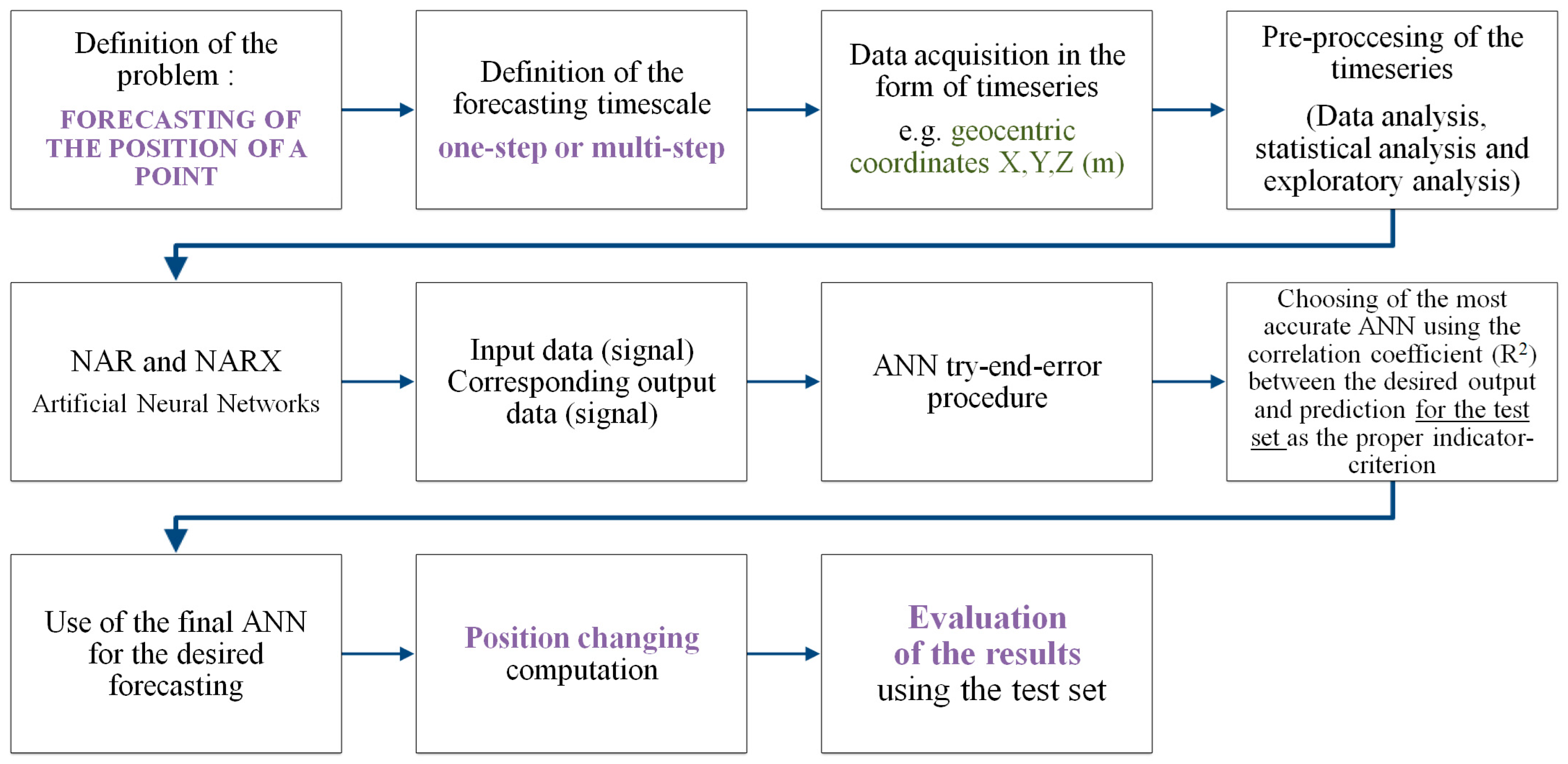
The first step is the definition of the examined forecasting problem. This means that the aim of the forecasting and the future use of the results need to be clear. In addition, it is useful to define the timescale (one-step-ahead forecasting or multi-step-ahead forecasting, namely short-term or long term) of the desired forecasting.
The problem, which the methodology deals with, is the forecasting of the position of a point in a future time. It is important to mention that the desired forecasting depends on the available data set. No change in the position of a point of the order of a few mm can be forecasted if no such displacement is recorded in the existing data, i.e., if the geodetic instruments and methods, which collect the data, cannot detect such a displacement.
Thus the basic steps of the methodology are: Problem definition → finding the available data in time series form → preliminary data analysis (data pre-processing) → ANN definition → evaluation → production of forecasts. These steps are presented in
Figure 1.
2.1. Preliminary Data Analysis (Data Pre-Processing)
This stage is of a great importance since it has a significance role in the accuracy of the results. Through this process the mechanism that produces the timeseries can be found.
The first test is to identify if the timeseries follows a known distribution. This test can be performed either by the Kolmogorov-Smirnov test [
28] or its variation, the Anderson-Darling Gof (goodness of fit) test [
29]. If the timeseries does not follow a known distribution, then it is possible to transform it. The transformation that can be used for this purpose is the Box-Cox [
30,
31], so that the abnormal timeseries becomes almost normal. Johnson transformation can also be used as an alternative method [
32].
Additionally, the statistical analysis (statistics) of the timeseries is then used to find statistical measures. The computational measures, which are used, are: the mean, the maximum and minimum values, the standard deviation, the covariance, the autocovariance, the correlation and the autocorrelation.
The next step is to find the qualitative features and the timeseries analysis of the major components. At this stage is checked if the timeseries is stationary or have any trend, seasonality, cyclicality or randomness. To convert the timeseries from no stationary to stationary, the diffusion method is used to calculate either the first or the second differences.
Finally, it is sometimes useful to analyze the frequency of the timeseries in order to find some information that is not immediately apparent in the original signal (timeseries). Then there is the possibility to use some mathematical transformations such as the Fourier Transformation, the Fourier Short-Time Transformation and the Wavelet Transformation, with the ultimate goal of retrieving some additional useful information.
It is then necessary to manage:
the missing values presented in the timeseries,
the possible zero values in the event that it is known that they should not exist,
the duplicate recordings that may exist and
any unusual observations (outliers) [
33].
With regard to the missing values likely to be presented in the timeseries, if they involve long periods of incomplete data, an effort should be made to find these values from other sources. If there are individual cases (not continuous time) and when no seasonal behavior has been observed from the plot of the timeseries, this missing value (or an unexpected zero value) is defined as the mean of the previous and the next value. In the case of duplicate recordings, they must be detected and deleted.
The most complex case is the existence of outliers. The difficulty of this case lies in detecting these values not in an optical way but in a mathematical way that can be automated. Once those individual values are found, they are replaced by the method used in the previous cases, if that is possible. A definition of the outliers is given as follows [
34]: “
An outlier is a residual which, according to some test rule, is in contradiction to assumptions on the stochastic properties of the residuals”.
There are several methods for finding outliers such as the Z-score, modified z-score, tucked method, boxedot, MADe method, Median rule, and generalized ESD test [
35]. Each test should be checked by the researcher for its suitability for the problem under consideration [
36,
37].
2.2. Prediction Interval (PI)
When attempting to forecast a value of a phenomenon, the result always has an uncertainty and an ambiguity [
38], so it is necessary to define the forecasting interval.
Forecasting interval or prediction interval (PI) is defined as the interval within which the value is expected to occur with a specific probability (1–a) % [
39]. It is very important to estimate this interval, in order to finally find the most accurate forecasting method [
40].
The interval consists of an upper predictive limit (UPL) and a lower predictive limit (LPL) [
41]. In the international literature, they are referred to either as forecast limits [
42] or as prediction bounds [
43].
There is a parametric and non-parametric approach for estimating the forecasting interval. In the parametric approach, which was proposed by Box and Jenkins [
44], it is considered that forecasting errors
, meaning the series {
}, is independent and follows the normal distribution with zero mean and variance
. The forecasting error used concerns data that is not used when creating the model or applying a method and it is often referred as an out-of-sample forecast error. The PI, for a probability (1-a) %, is calculated by the following equation [
41,
45]:
where
denotes the appropriate (two-tailed) percentage of a standard normal distribution and the standard deviation of errors is calculated from the equation:
and
(bibliographically referred also as bias) where N is the number of the observations.
Thus, the prediction limits are as follows: and .
2.3. The Design of the Forecasting ANN
Since the problem relates to forecasting, so that the concept time information is used, the appropriate ANN is a Dynamic Neural Network.
In this work, the dynamic network decided upon by an extensive bibliographic study is a recurrent or feedback dynamic network (RNN), because they can process data sequences, time information in our case. They can simulate two kinds of memory elements, long-term and short-term.
In every kind of ANN, the synaptic weights can be considered as long-term memories. However, if the problem has a temporal dimension, some form of short-term memory must be integrated into the neural network. The simplest way to do this is with time delays.
RNNs also allow non-linear relationships to be found, between the elements of a time series. The most important is that these networks have the advantage of recognizing time patterns regardless of their duration. More specifically; non-linear autoregressive recurrent networks (NAR) are chosen for forecasting one time step, and non-linear autoregressive with eXogenous inputs (NARX) for multi-step forecasting.
In the case of NAR, the forecasting of the
element of the timeseries is made, using only d past values of that timeseries, according to the equation:
Similarly, in the case of NARX, the d past values of the same timeseries (
) and also d of another exogenous timeseries (
) are used, according to the equation:
The training of the ANN is done through supervised process based on prior knowledge of the right outputs. For this reason, a percentage of the historical data is retained at the end for evaluation and control of the results.
These networks produce a one-step-ahead forecasting only. In order to forecast a multi-step-ahead, a loop is added to the networks. That is, once the first forecast is made, it returns to the network as an input to produce the next forecast, and so on. Therefore, the network based on its own outputs (forecasted values), also forecasts the following future values.
In order to select the most suitable final network, after its general architecture has been decided, various tests of ANN’s implementation are carried out, with the main objective of finding the one that will achieve the best results for forecasting. The basic principle used is that of validation by varying the hyper-parameters of the network: the number of hidden layers, the number of neurons of each hidden layer, the learning algorithm, the activation function of the hidden and exit neurons, and the number of delays.
For this methodology the Min-Max normalization is proposed, in order to normalize the values between low = 0.1 and high = 0.9 using the following equation.
where
and
are the min and the max value of the original timeseries
The available historical data (timeseries) is proposed to be separated in chronological order by using the following percentages: training set 70%, test set 15% and validation set 15%.
The training algorithm, which is found to be appropriate, is the Bayesian regularization and the training function is the log-sigmoid (logsig) function. The use of only one hidden layer is proposed in order to keep complexity low and training times small.
2.4. Forecasting Evaluation
Estimating the uncertainty of the forecasts is an integral part of the forecasting process. In order to evaluate a forecast, the results obtained must be compared with the actual values, which are already known. Thus, some statistical indicators or other evaluation criteria are used.
The evaluation criteria which are proposed are the Mean Square Error (MSE), the Root of the Mean Square Error (RMSE), the Mean Absolute Error (MAE) and the Coefficient of Determination (R
2) [
46].
R2 is used as one of the usual evaluation methods is to perform a linear regression in order to check if the selected method has a good performance during the evaluation phase. This index is interpreted as the percentage of the variance of the values of the dependent variable (i.e., the predicted values) from the values of the independent variable (i.e., the actual-known values).
R2 index measures the amount of variance in the target variable that can be explained by the model. In some cases, it is necessary to quantifying the error in the same measuring unit of the variable. This problem is solved by the use of RMSE. The issue with RMSE and MSE, is that since they square the residuals they tend to be more affected by large residuals. However, MSE has the possibility to highlight possible extreme deviations. This is the most common index of error that shows the qualitative performance of the forecasting method. Obviously, it does not have the same units as the actual values and the forecasts, so instead of this RMSE is used.
To solve the problem with large residuals MAE can be used, as it averages absolute value of the calculated residuals. Taking the square root of the average squared errors has some interesting implications for RMSE.
MAE is a failure index of the forecast by its actual desired value. Absolute values are used, so the forecast trend is not taken into account. The main difference between using MAE or RMSE is that MAE assigns equal weight to all errors when calculating overall performance while, as it is referred above, RMSE gives greater weight to errors with greater absolute value. Thus, RMSE is never lower than MAE for the same data set. When both metrics are calculated, RMSE is by definition never smaller than MAE. Since the errors are squared before they are averaged; RMSE gives a relatively high weight to large errors. This means RMSE should be more useful when large errors are particularly undesirable. There are cases when MAE may be steady but RMSE may increase as the variance associated with the frequency distribution of error also increases [
47].
In order to define the accuracy of the forecasting the mean position change must be calculated. Specifically, a forecast can be considered as accurate if MAE is significantly smaller than the mean forecasted position change.
3. Case Study
GNSS data are used in numerous of studies for the monitoring of the points position in a construction or for the Earth’s crustal movements [
48,
49,
50,
51]. The main advantage is that these data are in timeseries form, which is necessary for the implementation of the methodology. The above mentioned and analyzed methodology was tested by using actual data, acquired by permanent GNSS stations.
Specifically, the case study was implemented by using data from the Earthscope-Plane Boundary Observatory (PBO), which collects archives and distributes data from a broad network of over 1000 GNSS and seismic sites located across the continental United States and Alaska. These data are freely and openly available to the public [
52,
53] and they are referred to long time period (from 2003 to 2016).
As the methodology suggests, non-linear autoregressive recurrent networks (NAR) were used for one step forecasting, and non-linear autoregressive with exogenous inputs (NARX) either for one step or for multi-step forecasting. In order to find all the hyper parameter of the final ANN a great number of tests were carried out. All the tested ANNs were consisted of one hidden layer and the activation function of the hidden and output neurons was the logsig function. The tests were initially differentiated in the following:
- -
the input data normalization interval [−0.8,0.8] or [0.1,0.9],
- -
the input data division method, into random separation (70%, 15%, 15%) or chronological (70%, 15%, 15%),
- -
the training algorism trainlm or trainbfg or trainbr.
From the above combinations, 12 test sets are created. Each test set eventually implements 12 separate ANNs which then differentiate into the following parameters:
- -
the number of hidden neurons: min = 5, max = 20, step = 5 (four combinations)
- -
the number of delays: min = 2, max = 82, step = 40 (three combinations)
Additionally tests were conducted for different input and output data, according to 14 different scenarios which are created for each i GNSS station (
Table 1).
Therefore, 12 test sets were created for each of the 14 scenarios. In each test set, 12 ANNs with different parameters are implemented and trained for each GNSS station. In total 2016 (12 test sets × 14 scenarios × 12 ANNs) ANNs were tested only for one step forecasting for each GNSS permanent station. Furthermore, the same number of ANNs were trained for multi-step forecasting, with the difference that in this case only NARX neural networks where used.
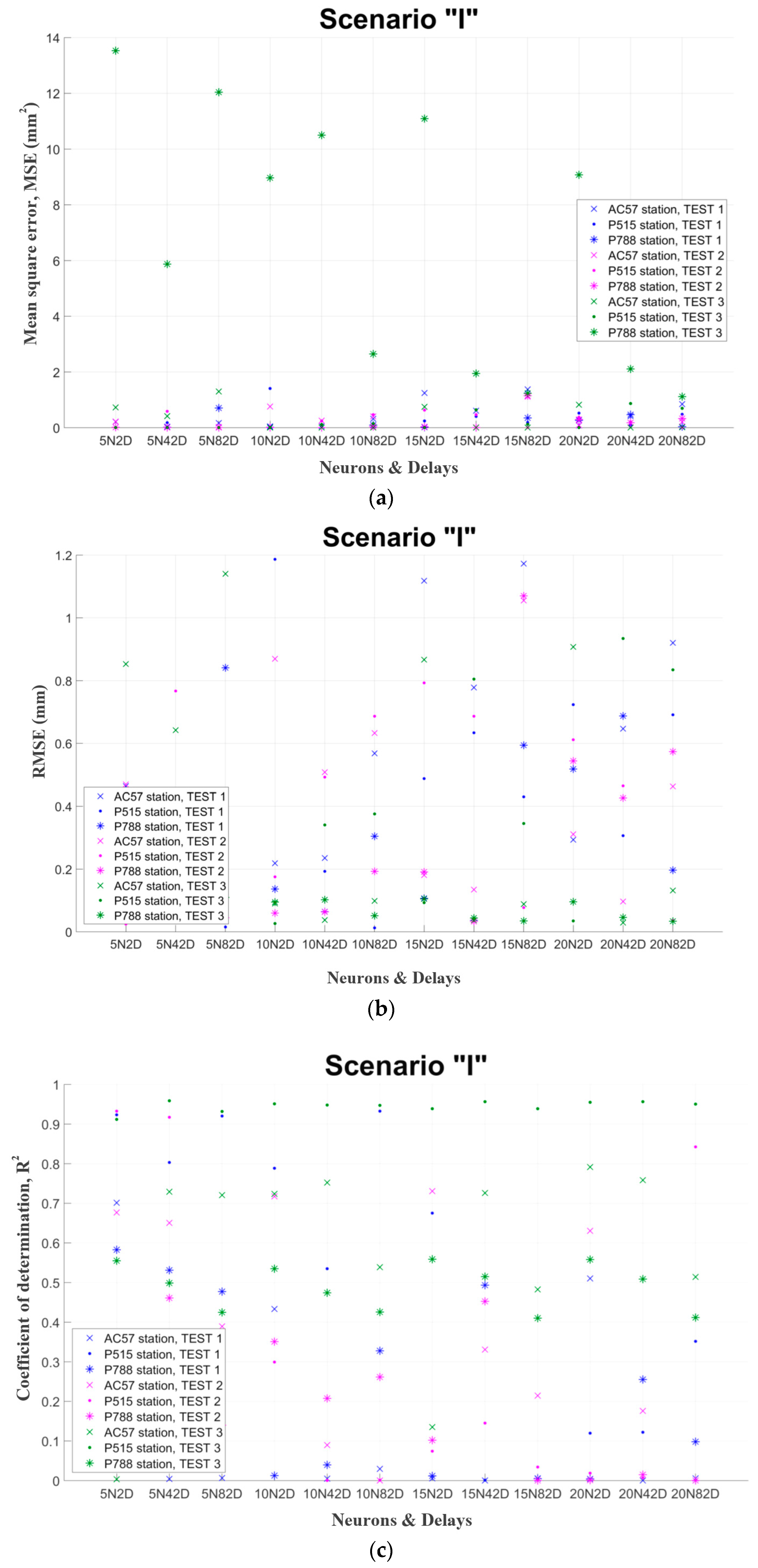
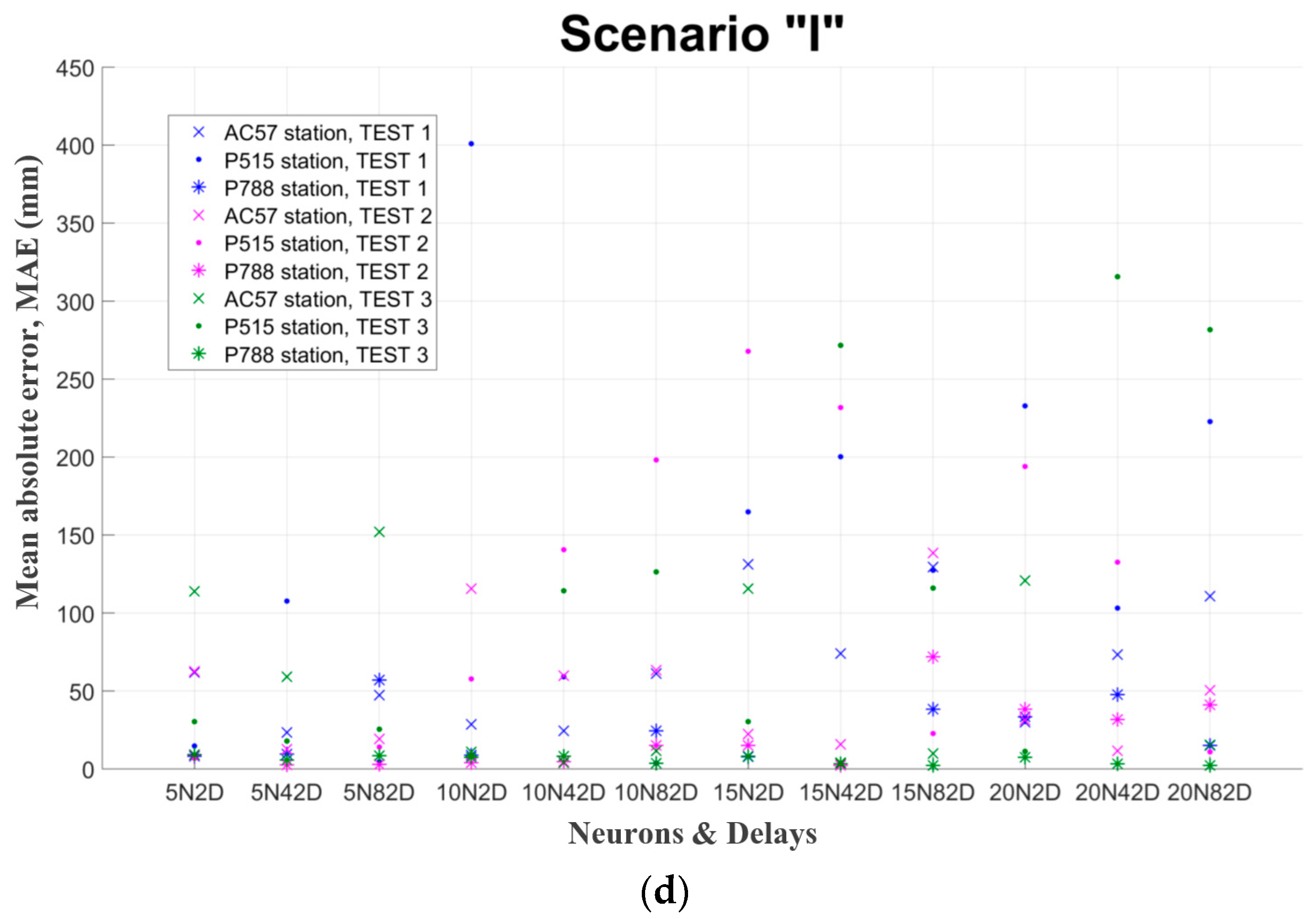
Figure 2 presents examples of the mentioned in paragraph 2.4 evaluation criteria for three random GNSS stations, namely AC57, P515 and P788. The final hyper-parameters are chosen after the assessment of those diagrams. Finally, the network, which has the smallest values (for the test set) in these criteria, is selected. Each GNSS station has different number of test set data, because this number depends from the original available data. However, in every case the test set is the 70% of the total available data. In particular, the exact number of the training set was ranged between 300 daily records and 2000 depending each GNSS station.
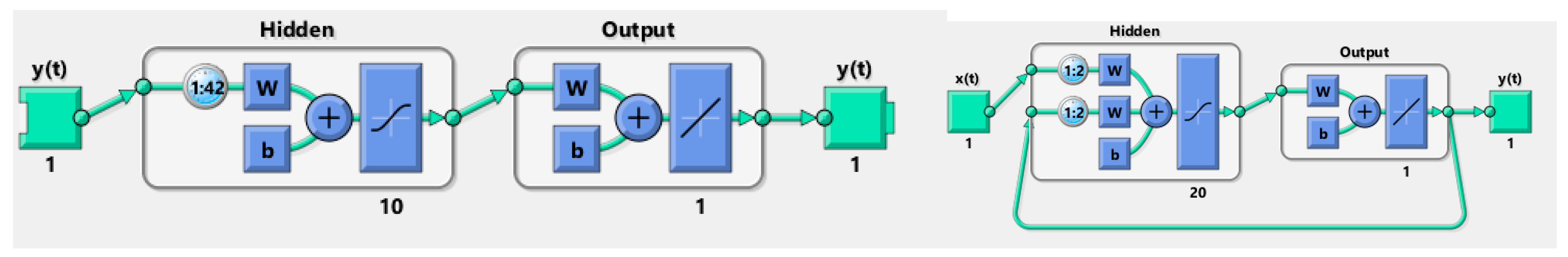
After all the above evaluation it was resulted that the best ANN for point position forecast: has as inputs and outputs separately the geocentric coordinates X, Y, Z (m) of each station (scenarios I, II and III). It consists of one hidden layer and has as activation function of hidden neurons and output neurons the logsig function. Data is separated in chronological order (70%, 15%, and 15%) and their normalization is in the range [0.1,0.9]. The training algorithm is Bayesian regularization. The number of hidden neurons is 10 and the number of delays 42 for one-step forecasts. While for multi-step forecasts there are 20 neurons and 2 delays.
The mean MAE of the 1000 GNSS permanent stations was calculated and presented in the following table (
Table 2).
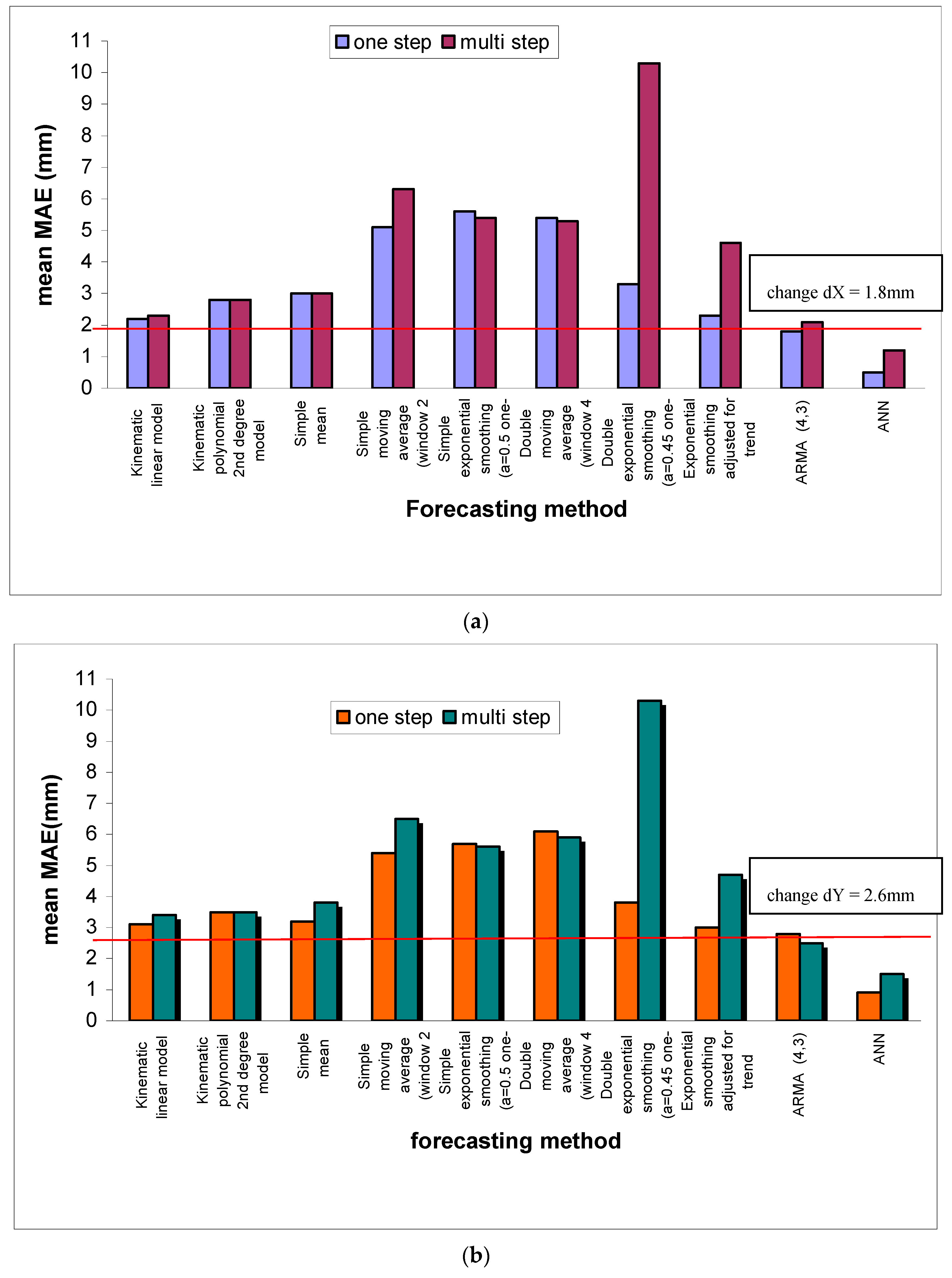
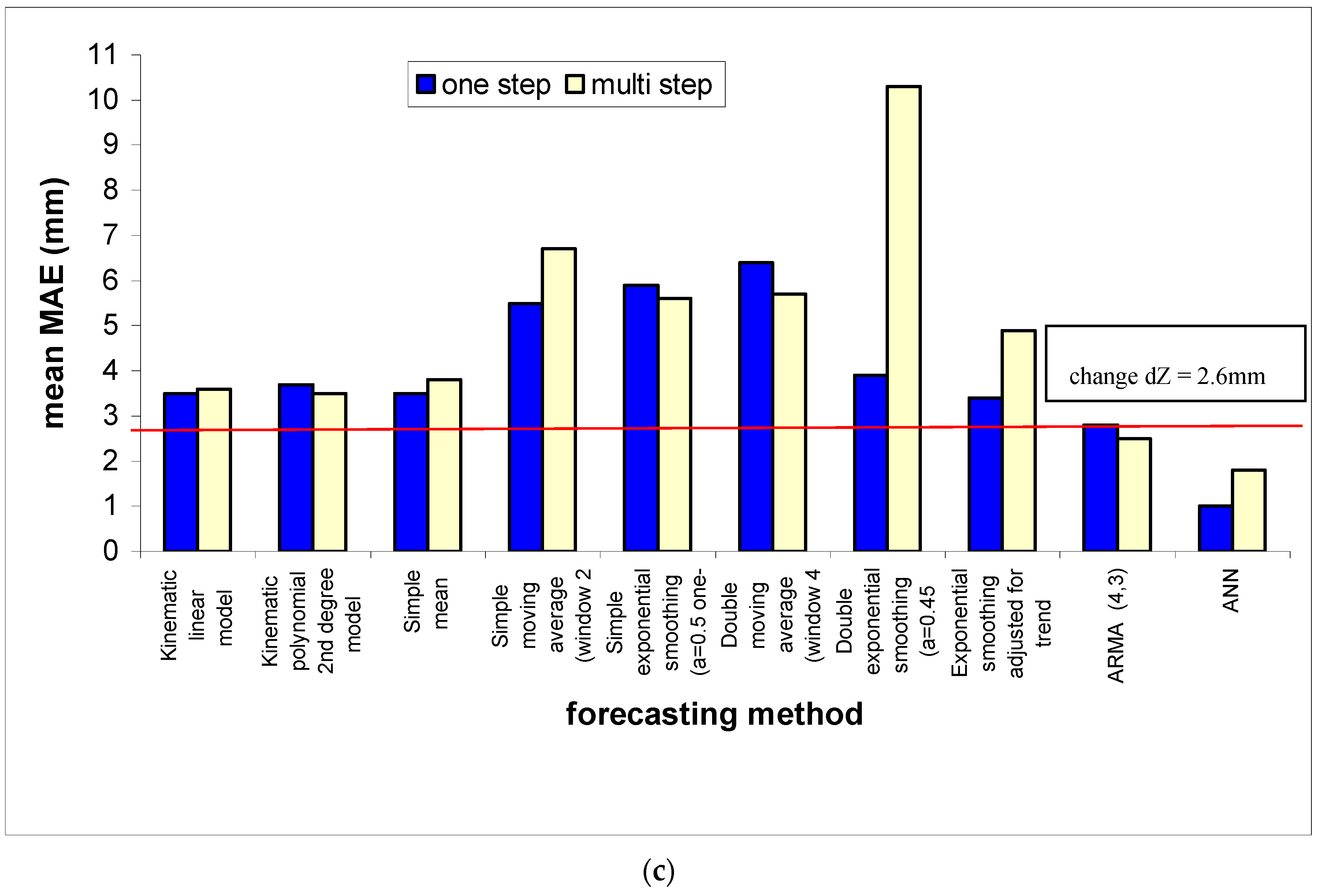
In addition some other conventional methods were used for the same purpose. The scope is to compare the forecasts generated by this intelligent method to those, which are provided by some other specific conventional methods. The nine conventional methods that were selected to be examined and compared are the following: Kinematic linear model, Kinematic polynomial 2nd degree model, Simple mean, Simple moving average, Simple exponential smoothing, Double moving average, Double exponential smoothing (Brown’s method), Exponential smoothing adjusted for trend (Holt’s method) and Autoregressive Moving Average Methods (ARMA). The comparative results of the chosen conventional methods and the proposed ANN are presented in the following
Figure 3.
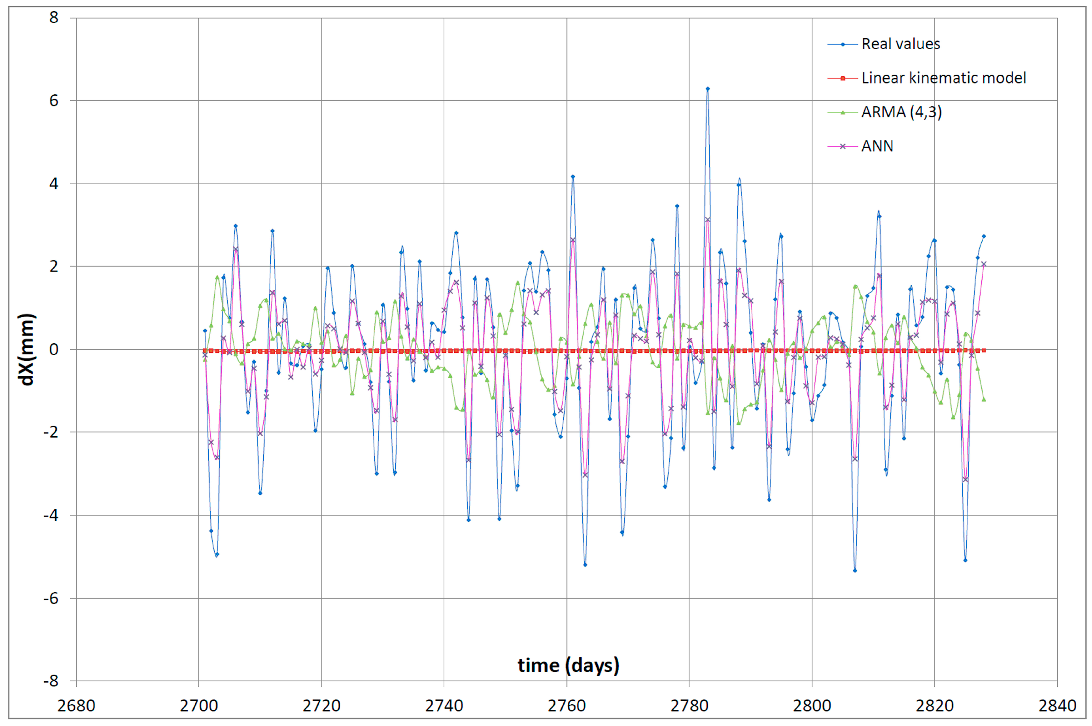
Additionally
Figure 4 illustrates the reliability of the ANNs forecasts relative to the two optimum, between the nine chosen ones, conventional methods (kinematic linear model, ARMA (4,3). It is obvious that the proposed ANN, especially in the case of short-term forecasts, is able to adequately forecast the size and the trend of the change of point positions. On the contrary, it is also evident that the two examined conventional methods have a significant deviation both in the forecast of the size and of the trend of the point positions change.
4. Discussion
The proposed methodology has been developed to solve the problem both for one-step-ahead (short-term) and for multi-step-ahead (long-term) forecasting.
To sum up, the ANN resulting as the best for forecasting the change of points position is a non-linear autoregressive NAR recurrent neural network and a NARX non-linear autoregressive with eXogenous inputs in the case of multi-step forecasting. Some preliminary tests on a sample dataset led to the following ANN design choices and training procedure:
It consists of one hidden layer and has “logsig” as an activation function of hidden and output neurons.
Separation of the data is done in chronological order (70%, 15%, 15%) and their normalization in the interval [0.1,0.9]
The learning algorithm is the Bayesian regularization backpropagation.
It is proposed the number of hidden neurons to be 10 and the number of delays 42 for one-step forecasts, while for multi-step forecasts 20 hidden neurons and 2 delays.
Finally, in cases where time series of geocentric coordinates X, Y, Z (m) are used, it is proposed X, Y, Z to be used separately as inputs and outputs.
The best ANNs for one-step and for multi-step forecasting are presented accordingly in the following
Figure 5.
The number of available data to be used is a very important factor in their training. As the number of data increases, the better the network will be “trained” and will therefore produce better results.
Big data management is very complex and requires special treatment. In such cases it is necessary to use automated techniques rather than optical means as in smaller volume and size data. Despite the difficulties, finding and using large amounts of information is a major asset especially when it comes to forecasting.
During training, special care must be taken to avoid the overfitting phenomenon. If the network is trained for too many epochs and/or in the entire dataset, we could observe small training error but lose the ability to generalize well, i.e., perform well on new, unseen data. Therefore, there is a possibility that there is a limit beyond which, while the training error decreases, the validation error increases. In this situation, the network may have memorized the correct results that arise from the education phase, but has not learned to generalize properly on new data.
As already mentioned, the proposed methodology is based on ANNs. The main drawback of their use is the large number of tests (try-and-error process) that must be carried out with all the possible different combinations of the hyper-parameters.
Therefore, in cases where the data is so many, a representative sample should be selected by which all the experiments will be carried out and, finally, the most suitable ANN will be proposed. The sample could be simple random, systematic or else quasi-random and finally stratified random depending on the available dataset.
Despite this disadvantage, the methodology gives more accurate forecasts compared to some other selected conventional-statistical forecasting methods (i.e., simple mean, simple moving average, simple exponential smoothing, double moving average, Brown’s method, Holt’s method, ARMA/ARIMA models) [
54].
5. Conclusions
ANNs have been introduced to the engineering sciences in general and Geodesy in particular. In recent years, an attempt has been made to investigate their use. Several of the geodetic applications in which the ANNs have been used to date have yielded very satisfactory results, giving even better results compared to classical methods for solving these problems. Applications mainly used are local geoid mapping, averaging of the sea level, coordinate conversion to reference systems, mobile mapping models, and so on.
This research, by using actual data, acquired by 1000 permanent GNSS stations, ascertains that the best forecasting results succeeded when simple scenario of input and output data are applied, namely when the forecasting is made separately for each coordinate X or Y or Z. This is concluded after 14 different scenarios results. Also the data separation in chronological order leads to better forecasts than the random separation.
The numerous available data permits to realize all the 12 test sets, which are created for each of the 14 scenarios and the 12 ANNs with different parameters in each test set, in total 2016 ANN. This gives the opportunity for reliable conclusions. MAE is proved to be a satisfied and unbiased index as assigns equal weight to all errors when calculating overall performance, so it provides a real estimation of the forecast uncertainty. The multi step forecast provides always twice greater MAE than the one step ahead.
The ANN can forecast a point’s position change of the order of 2 mm with MAE in the order of 0.5 mm, while the optimum convention method, ARMA model (4,3), with MAE 1.8 mm. Moreover the most significant is that it gives not only the right size of the position change with adequate accuracy but also it indicates the right trend of the position change vector.
As far as ANNs are concerned, this is a modern and very attractive intelligent technique. For this reason, implementing an ANN to solve any problem is an interesting and original alternative. However, a try-and-error process must always be followed during the implementation process. The more testing done, the more complete the work is to investigate the use of ANNs for any problem. This means that it takes a lot of time and a lot of computational power until one gets the desired result.
The documentation and suggestion of a particular ANN and all its hyper-parameters arises after each application, which is another significant disadvantage. ANNs are a data driven method, so the architecture and hyper-parameters found to be optimal in a dataset, in the general case won’t be optimal for another dataset.
This methodology, which is based on ANNs is accurate, stable and general and can be used in order to forecast the changing of points’ position. It also gives accurate and reliable results compared to some selected classical-conventional methods.


