Population Synthesis Handling Three Geographical Resolutions


Department of Civil, Geo and Environmental Engineering, Technical University of Munich; Arcisstr. 21, 80333 Munich, Germany
*
Author to whom correspondence should be addressed.
ISPRS Int. J. Geo-Inf. 2018, 7(5), 174; https://doi.org/10.3390/ijgi7050174
Submission received: 4 April 2018
/
Revised: 26 April 2018
/
Accepted: 30 April 2018
/
Published: 4 May 2018
Abstract
:In this paper, we develop a synthetic population as the first step in implementing an integrated land use/transport model. The model is agent-based, where every household, person, dwelling, and job is treated as an individual object. Therefore, detailed socioeconomic and demographic attributes are required to support the model. The Iterative Proportional Updating (IPU) procedure is selected for the optimization phase. The original IPU algorithm has been improved to handle three geographical resolutions simultaneously with very little computational time. For the allocation phase, we use Monte Carlo sampling. We applied our approach to the greater Munich metropolitan area. Based on the available data in the control totals and microdata, we selected 47 attributes at the municipality level, 13 attributes at the county level, and 14 additional attributes at the borough level for the city of Munich. Attributes are aggregated at the household, dwelling, and person level. The algorithm is able to synthesize 4.5 million persons in 2.1 million households in less than 1.5 h. Directions regarding how to handle multiple geographical resolutions and how to balance the amount and order of attributes to avoid overfitting are presented.
1. Introduction
Synthetic populations are used in transportation modeling when individual records of households and persons are not available due to privacy reasons, insufficient resolution, or missing attributes. Within the context of transportation modelling, population synthesis is the process of creating a representation of a complete, disaggregate population by combining a sample of disaggregate members of a population in a way as to match key distributions for the entire population [1]. Key distributions—also known as control attributes—can be at the household level, such as household size, at the person level, such as gender, age or employment status, or at the dwelling level, such as construction year or living space. Moreover, control attributes can be aggregated at different geographical resolutions, such as boroughs, municipalities, or counties.
Synthesizing a population has two main phases: optimization (fitting) and allocation. The first phase fits a disaggregate sample of agents (microdata) to aggregated constraints (control totals), while the second phase replicates actual agents for the synthetic population using a probabilistic selection [2]. While the procedure on the second stage is usually the same across population synthesizers and relies on Monte Carlo sampling, there is a broad range of procedures for the first stage.
There is an ongoing debate about which procedures and enhancements are best suited at the optimization phase. As seen in Table A1, the Iterative Proportional Fitting (IPF) procedure is a well-established algorithm for fitting [1,3,4,5,6,7,8,9,10,11,12,13,14,15,16,17]. This method, first proposed by Deming and Stephan [18], identifies weights for the microdata iteratively by adjusting an n-dimensional array until every dimension matches to the control totals. The same method is often called matrix balancing in computer science or RAS method in input-output analysis. The main disadvantage of the procedure is that it can only handle one level of aggregation (person or household) and geographical resolution (municipality or county) at each time. Some authors enhanced the procedure by: substituting the n-dimensional array with sparse lists to accommodate a large number of control attributes without exponentially increasing computational requirements [7]; using two-step IPF to accommodate person level and household level attributes in sequence [11]; incorporating more heterogeneity into the initial seed [17,19]; and combining IPF with spatial microsimulation [15] or reweighting IPF results using Iterative Proportional Updating (IPU) [17]. Recent work has evolved IPF into IPU, which calculates a set of weights for each one of the microdata records in an iterative approach. IPU is capable of closely matching household-level, dwelling-level, and person-level control totals at the same time [20] and it can accommodate control attributes defined at municipality-level and county-level simultaneously [21]. As with IPF, IPU is from the static family of models. Other procedures that can handle person and household-level attributes are entropy maximization [16,22,23], hierarchical IPF [24,25], combinatorial optimization [26,27], Monte Carlo Markov Chain [27,28], Hidden Markov Models [29], or multinomial regression models [30,31]. Most of the procedures are compared to IPF and usually tend to better match observed distributions in multiple dimensions, although the convergence time can be very high [26].
In terms of control attributes, all studies for transportation engineering include at least household size, age, and gender, as summarized in Table A2. Employment status has been included at the household [4,5,11,21,27] or person level [8,13,26,31,32,33]. While household income is available for most of the studies in the United States and Canada [4,7,9,10,11,20,21,22,26], it is commonly not included in European countries and Australia [8,13,23,27,32]. Other variables are the number of cars, number of children, type of dwelling, or ethnicity. Dwelling attributes are less common, with only a few studies including dwelling tenure [4,9,34] or dwelling type [4,11,32].
The aim of this work is to synthesize the population of the greater Munich metropolitan area. This paper does not intervene in the methodological debate by comparing performance of alternative procedures but rather gathers alternative procedures available and selects one suitable to the case study needs. The available data is limited in several respects, which triggered our need to create a new multiresolution solution. Firstly, person and household attributes are aggregated at the municipality level, but most dwelling attributes are aggregated at the county level. Secondly, the German administrative division classifies the city of Munich as a single municipality-county of 1.3 million inhabitants in 0.7 million households. A higher resolution is required to synthesize demographic and dwelling differences across boroughs. Thirdly, the data do not cover all attribute dimensions of households, individuals, and dwellings that the model requires. Specifically, data on individual income, car availability, land price, or number of bedrooms are missing. The first and second constraints lead to implementing one optimization procedure that can enable control at household, dwelling, and person levels simultaneously and can deal with different geographical resolutions in a reasonable amount of time. The third constraint is not fundamental and results in having a few uncontrolled attributes that are directly copied from the microdata.
2. Materials and Methods
The algorithm builds on several of the methods and techniques that have been introduced thus far in the field of population synthesis and expands it to three geographical levels. The method includes three stages: (1) selecting geographical resolution and scales of analysis; (2) optimization; (3) allocation. The following subsections will describe each stage and the application.
2.1. Selecting Geographical Resolution and Scales of Analysis
Two main data items required to synthesize populations are individual household structures (or household microdata) and aggregate distributions at a certain geographical resolution (or control totals).
Household microdata is provided by many statistics bureaus in the form of the microcensus. It includes basic socioeconomic information, current and previous employment, and location. Control totals are usually available at statistics bureaus. The data can be aggregated to several geographical resolutions: borough, municipality, county, state, or nationwide.
After data were collected, we selected attributes as control attributes. Control attributes must be meaningful for the model, included in both databases, and have equal or comparable stratifications in both databases.
2.2. Optimization: IPU with Three Geographical Resolutions
The optimization uses Iterative Proportional Updating (IPU). It was proposed by Konduri et al. [21] for two geographical resolutions, and it was expanded for this research to three geographical resolutions. The IPU procedure consists of adjusting the set of weights for each household of the microdata to minimize the error between control totals and calculated distributions of each attribute for each geographic resolution.
Before starting the IPU procedure, it is required to summarize each microdata record according to the categories of the control attributes. The result is stored in the frequency matrix. The frequency matrix shows the household and dwelling type and the frequency of different person types within each household for the sample. The dimension of the matrix is N × M, where N is the number of households in the microdata and M is the number of control attributes (household, person and dwelling type).
The set of weights is provided at the lowest geographical resolution. An initial set of weights is set to one. In the next iterations, weights are updated after considering each control attribute. All attributes, regardless of whether they are household, dwelling, or person type, are treated equally. Weights are only updated in the households where the frequency of the control attribute is different than zero. Attributes at the lowest geographical resolution (i.e., municipality) update only the weight of one record, while attributes at the higher geographical resolution (i.e., county) update a set of weights of all nested areas (i.e., municipalities or boroughs).
After all control attributes are considered, we calculate the relative difference in absolute difference between control total and calculated distribution for each attribute. The average error is compared to the previous iteration. If the absolute difference of average deviation values between two full iterations satisfies a set of tolerance criteria, the algorithm stops updating household weights. The default threshold is set equal to 0.01% and can be modified by the user. Average absolute relative difference across all constraints has been used previously by Ye et al. [20] and Konduri et al. [21] in the original IPU procedure and by others [3,5,23,31,35]. Other indicators for goodness of fit include standardized root mean square error [7,11,24,27,36], difference on counts [1,8,10], or error percentages [9]. Additional stopping criteria include the maximum number of iterations (default value set to 1500) and average error threshold (default value of 1 × 10 − 7). The process converges after several iterations depending on the number of control attributes and number of municipalities within one county.
Table A3 shows the pseudocode for the IPU with three geographical resolutions and two aggregation levels.
2.3. Allocation: Monte Carlo Sampling
To generate the synthetic population, households of the microdata are randomly drawn based on their weights. Once a household is selected for the municipality, it is allocated to a traffic analysis zone (TAZ) within the municipality or borough. The zone system nests TAZs within the municipal regions respecting municipal boundaries. The probability for each TAZ is the ratio between the population in the TAZ and the total population on the municipality.
The value of control attributes is directly copied from the microdata into the synthetic population.
Finally, we computed the absolute difference between the generated population and control totals. The goodness of fit of the allocation is evaluated as the average relative error of the control attributes at the highest-ranking geography (i.e., county).
2.4. Application
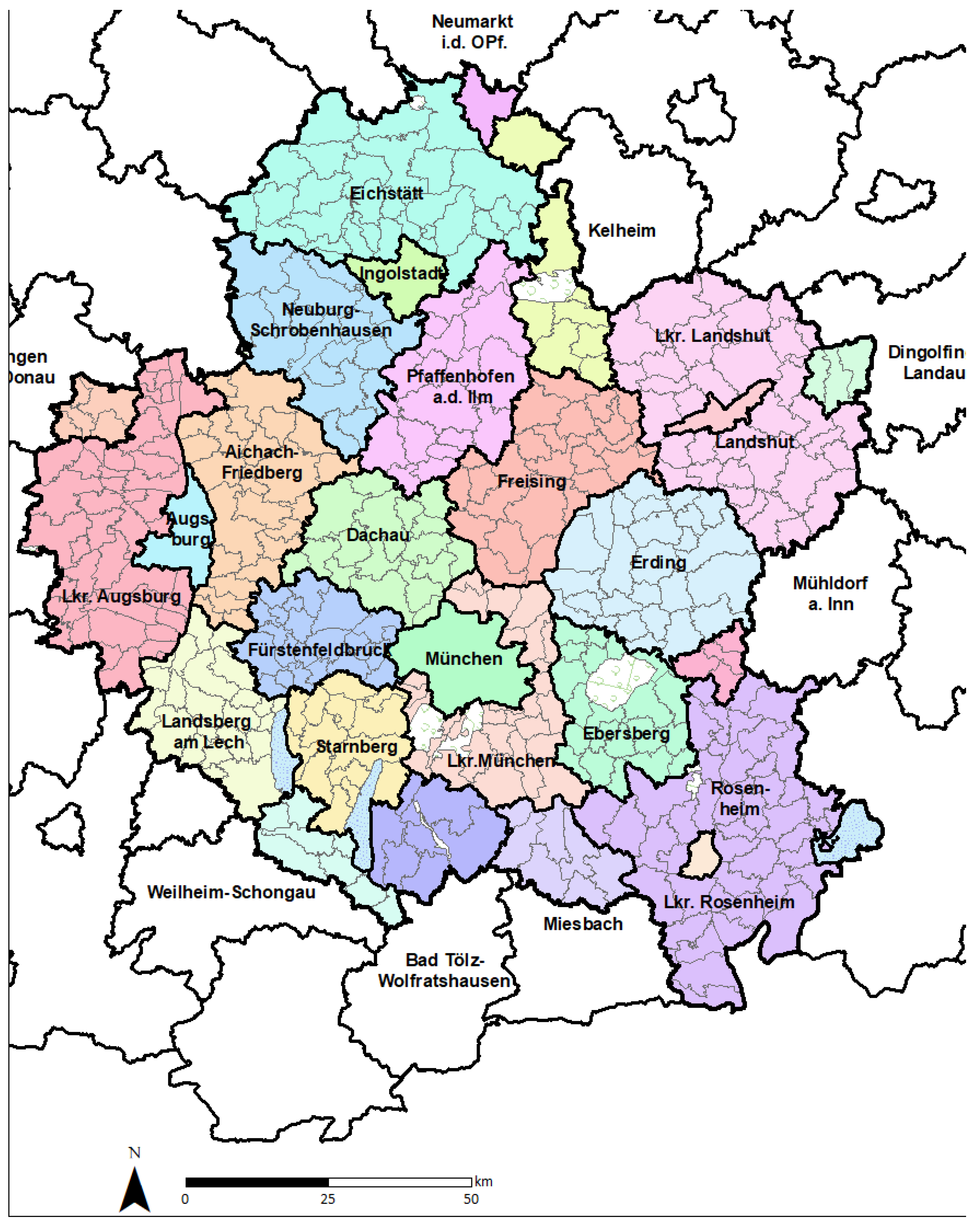
We applied our approach to the greater Munich metropolitan area (Figure 1). The region includes the cities of Munich, Augsburg, Ingolstadt, Landshut, and Rosenheim and their respective suburbs to cover the large commuting shed of the Munich region. The delineation of the study area was defined by the share of commuter flow into these five central cities. Municipalities were included in the area if at least 25% of workers commute to one of the central cities. The area includes a population of 4.5 million living in 2.1 million households. It has 444 municipalities distributed in 28 counties. The number of municipalities by county varied from 1 to 46.
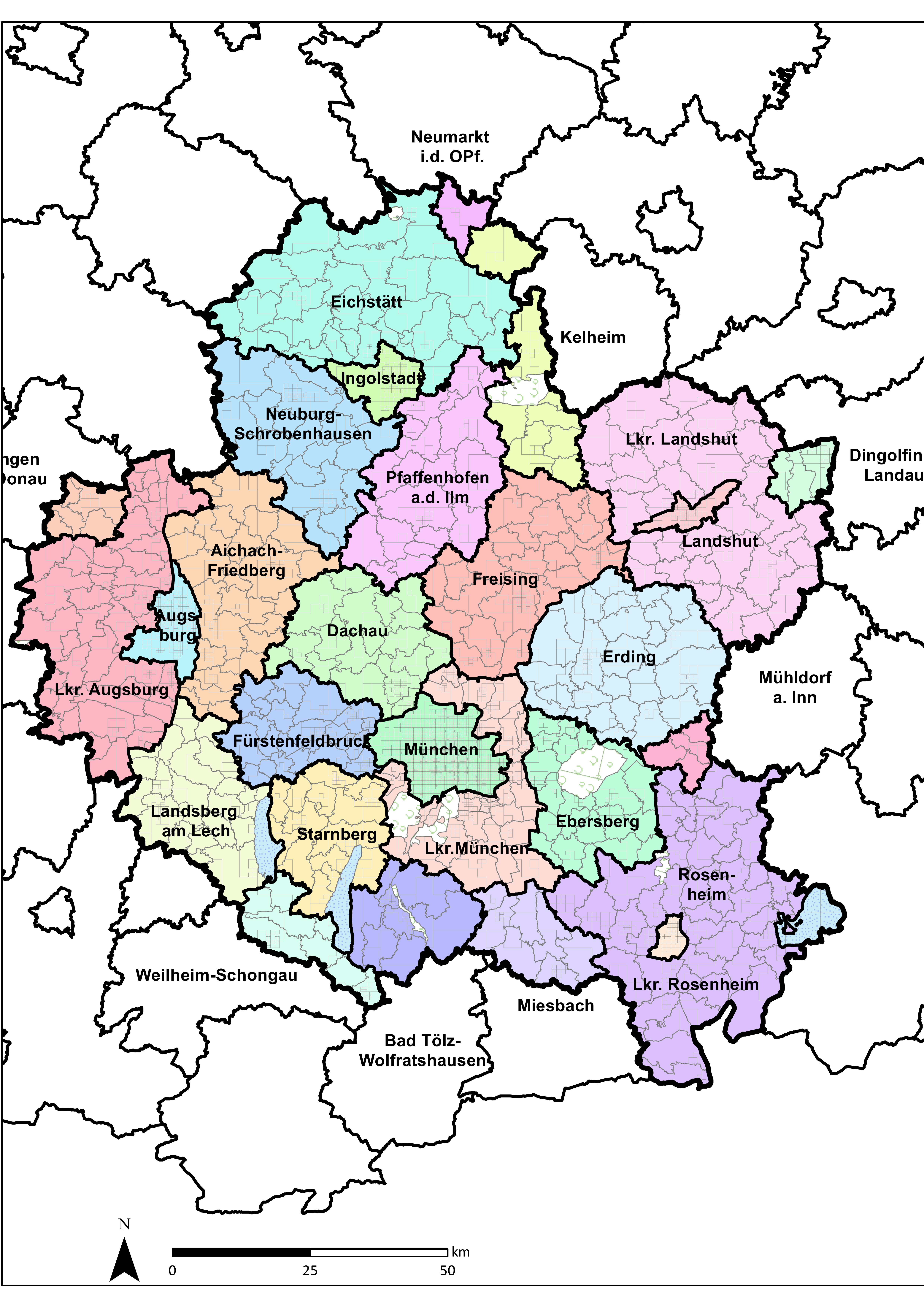
After delineating the study area, municipalities are divided in Traffic Analysis Zones (TAZs) using a gradual raster-based zone system [37]. The total number of TAZs is 4950 (Figure 2). Twenty-nine percent of the population lives in the city of Munich itself, while the average population per municipality is below 10,000. Therefore, a higher spatial resolution was created for the city of Munich than for other less populated municipalities.
The German household microdata was purchased from the German State Statistical Office. Due to privacy considerations, individual records are anonymized and not geolocated. In fact, the only geographical resolution of the reference is the state of residence (e.g., Bavaria). Control totals are available online at the German 2011 Household Census [38], the GENESIS Online database [39], the Census Hub [40], and the website of the city of Munich [41].
Based on the available data in the control totals and microdata, we selected 60 control attributes: 47 attributes at the municipality level and 13 attributes at the county level. For the city of Munich, we selected 14 additional attributes at the borough level. Table 1 summarizes the control attributes by type and geographical resolution.
The land use/transport model for which this synthetic population was generated requires other attributes that are not in the microdata, such as person income, person workplace, dwelling monthly cost, dwelling quality, or number of cars on the household. They are obtained from other submodels, such as car ownership model or land price model, and assigned by Monte Carlo sampling.
3. Results
This section presents the results of the synthetic population for the greater Munich metropolitan area. We analyze the differences between the aggregate distributions and the resulting synthetic population by: (1) geographical resolution and (2) attribute.
The optimization phase is deterministic, but the allocation phase produces slightly different model runs every simulation due to the random seed used while sampling. To provide some impression of the range of the sampling error, we ran the allocation five times. The average result of the five runs and the standard deviation between the five model runs are indicated.
3.1. By Geographical Resolution
Firstly, we analyzed the average error of control attributes at the municipality level (Figure 3). We took the absolute value of each control attribute’s error to calculate the average error by municipality. The errors after the optimization are shown in green, and the errors of the allocation are shown in orange. The errors after the optimization phase are generally below 6%. In fact, only 7 out of 444 municipalities had an average error higher than 6%. Those municipalities are located in large counties containing 46 and 23 municipalities, respectively. Additionally, some of the municipalities had a higher concentration of students or retired persons living in large households, which were scarcely observed on the microdata. The microdata seemed to underrepresent selected combinations of attributes, making it difficult to match all control totals very well.
The errors of the allocation phase are, as expected, highly dependent on the size of the municipality. In small municipalities, it is likely that many weights are near zero. Microrecords are sampled proportionally to their weights an integer number of times. The “law of large numbers” generally compensated the error on the attributes for a large number of draws, but it led to lower accuracy for small municipalities with a small number of draws, given the high number of possible combinations of attributes. In this sense, the size of the municipality, the number of microrecords, and the number of combinations of attributes should be balanced. In our case study, the balance was produced for municipalities with 5000 inhabitants or more (asymptote in Figure 3).
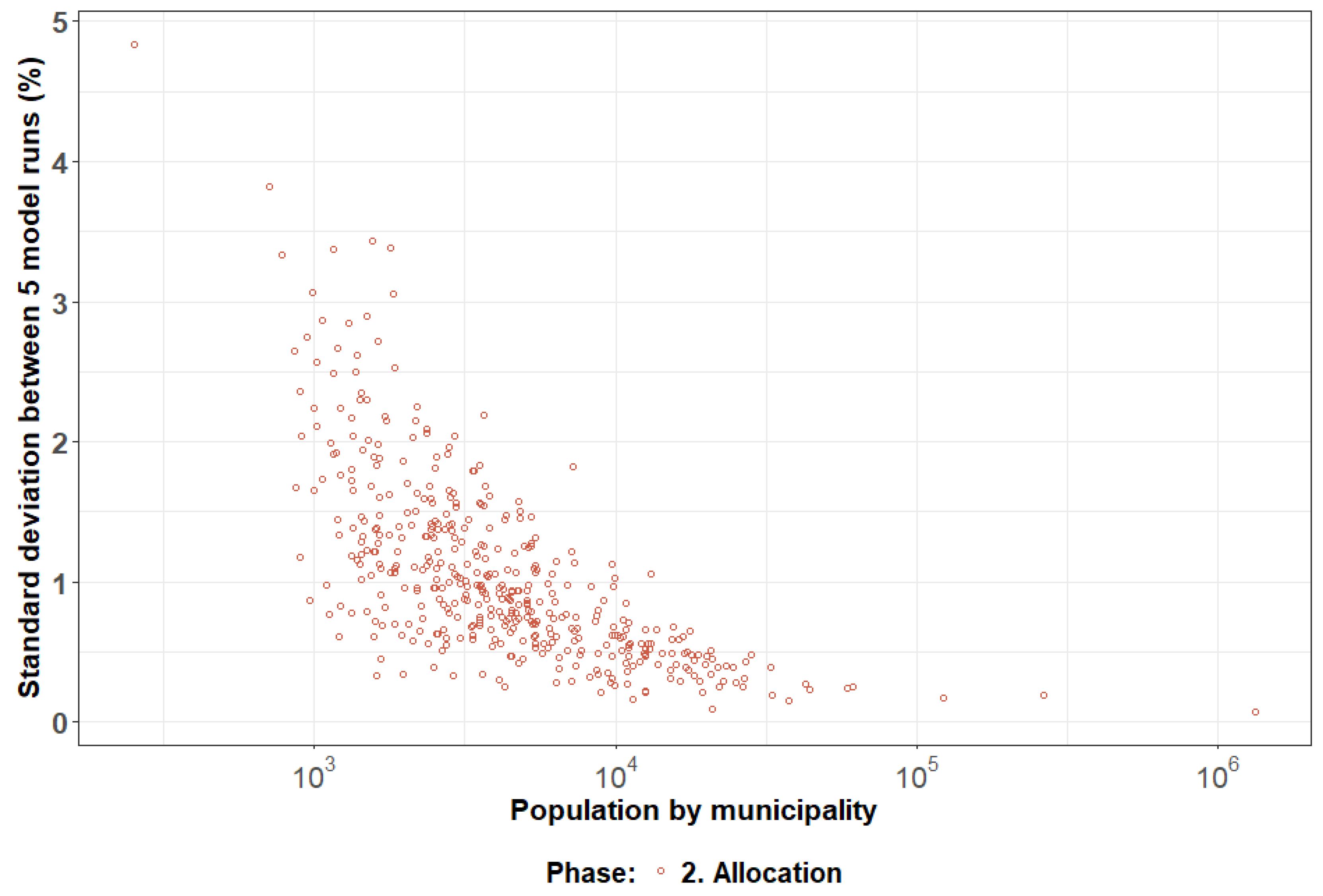
The standard deviation between the five runs is also highly dependent on the size of the municipality (Figure 4). The standard deviation is generally lower than 1% for municipalities higher than 10,000. The optimization phase is deterministic, and therefore the deviation in five runs is equal to zero. As a consequence, only the allocation phase is plotted in Figure 4.
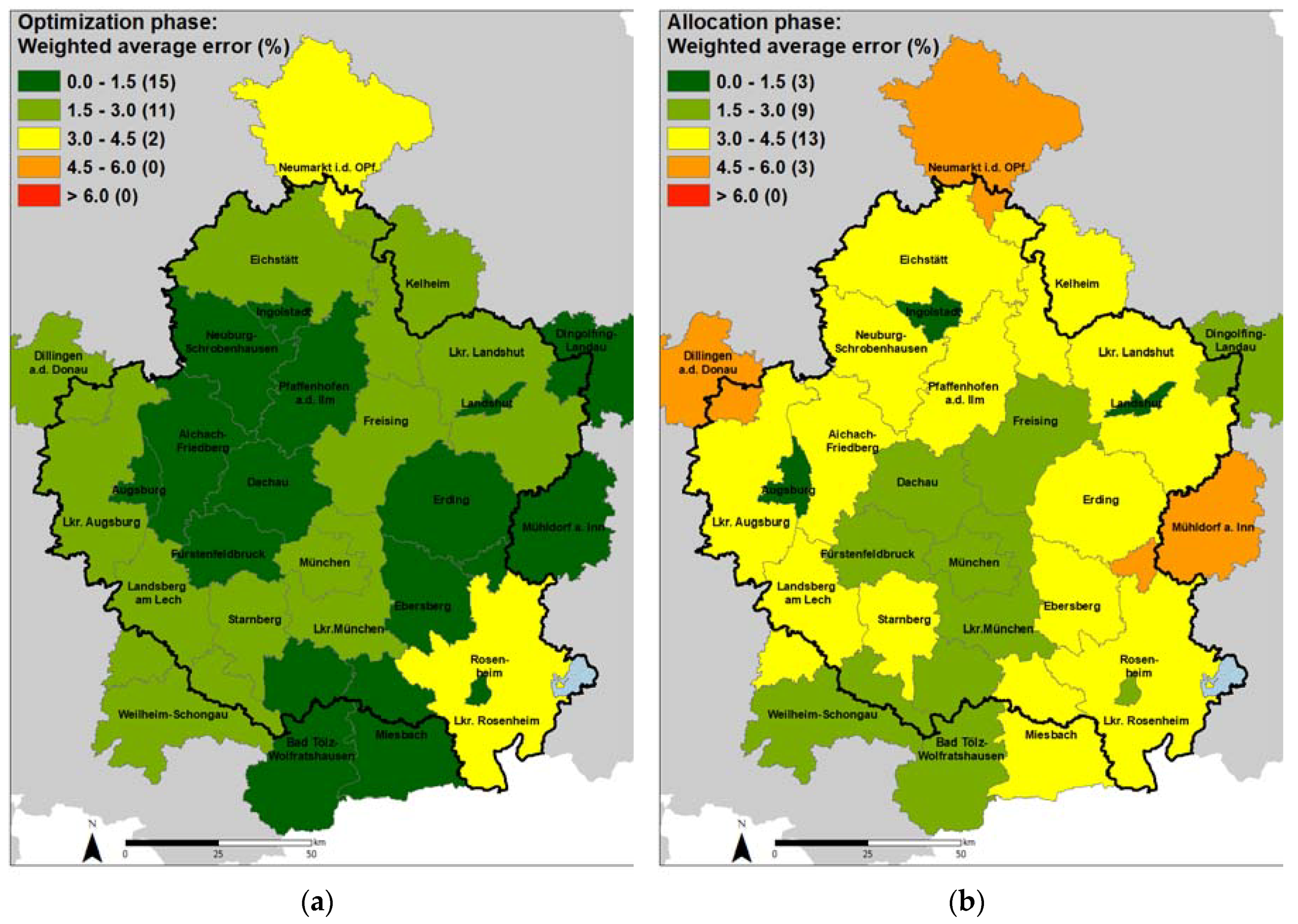
Secondly, we analyzed the errors at the county level for all attributes (Figure 5). Given the size dependency of the allocation error, the average error at the county level was calculated weighting the municipality error by its population. Weighted average error was used at the optimization phase as well for consistency.
After the optimization phase, the majority of the counties had a weighted average error lower than 1.5%, and only two counties exceeded 3%. Not surprisingly, the weighted average error increased during the allocation phase. Rural counties with smaller municipalities presented the largest weighted average errors, although they were below 6%. Compared to the municipality level, the weighted average error at the county level is lower. The lower error of measurement for the larger zones is only a natural effect of the scale-dependent accuracy of geoinformation, perhaps due to spatial autocorrelation of the data and that at the county level, the number of microrecords is multiplied by the number of municipalities within the county, having a bigger sample to distribute the control totals.
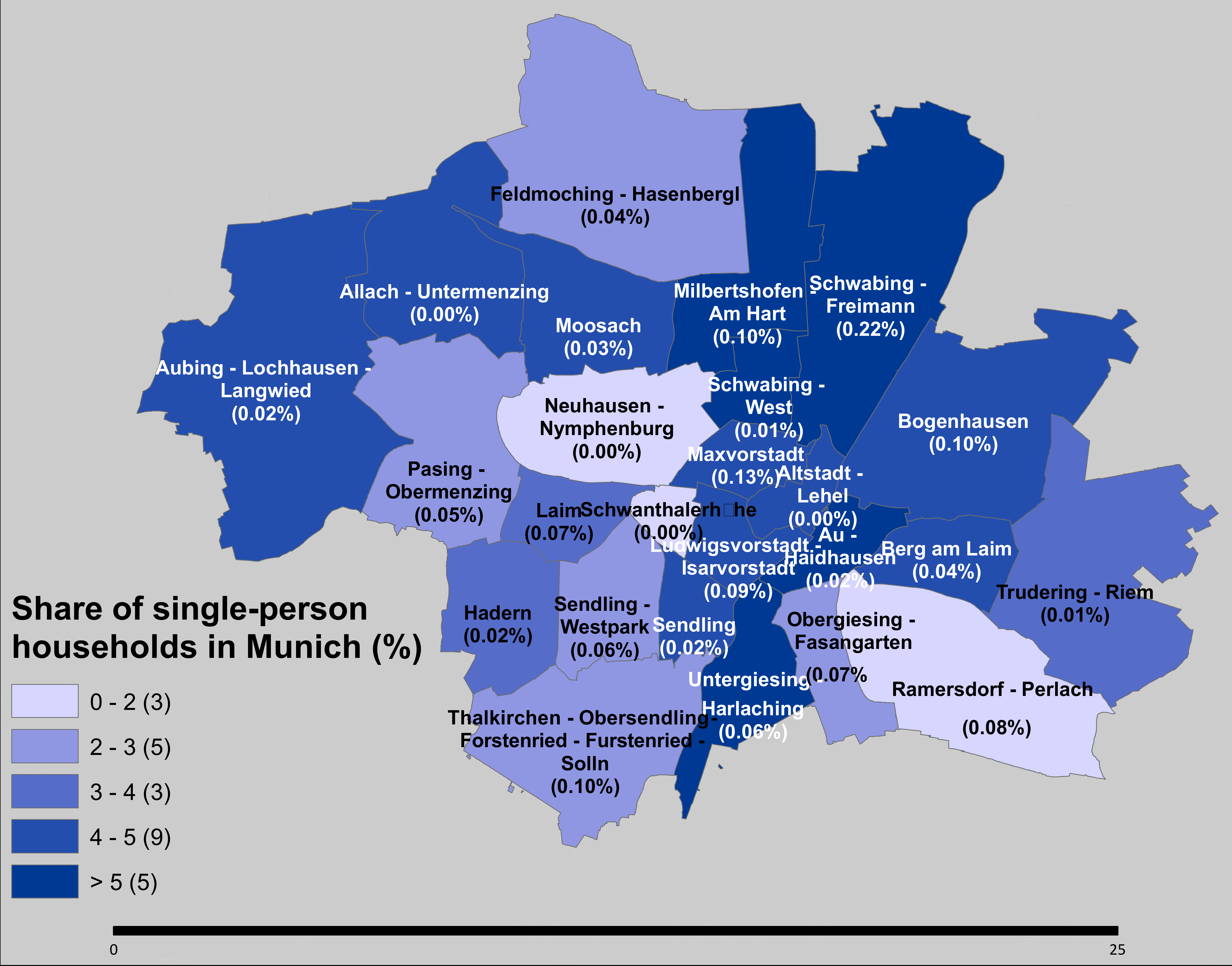
Finally, we analyzed the results for the city of Munich at three geographical resolutions: county, municipality, and borough. The error for the city of Munich was 2%, slightly higher than other large cities. The attribute with the highest error is single-person households, which provided an average error of 10%, similar across all boroughs. The error is produced due to inconsistencies between borough and municipality control totals, as the total number of single-person households in Munich differs from 368,447 at the municipality level to 410,993 as the sum of the boroughs. The difference is around 10%, which is the same result obtained from the algorithm.
Figure 6 shows the share of single-person households across Munich boroughs and the difference between control totals and the results after the optimization. The differences in absolute value are below 0.2%, providing practically the same distribution of the attributes across all boroughs. Therefore, the sole analysis of the error could be misleading when control totals at different resolutions are not consistent.
3.2. By Attribute
The weighted average errors (in absolute value) and deviations for household, dwelling, and person attributes are summarized in Table 2, Table 3 and Table 4, respectively. We took the absolute value per municipality and calculated the weighted average error, as in the previous analysis. In all the cases, the errors at the allocation phase are higher than the errors at the optimization phase. Deviation at the optimization phase is equal to zero because the procedure is deterministic.
The error in the total number of households is equal to zero because the method adjusted weights to match that number. During optimization, the total number of households was the last attribute to compute. As a consequence, the final weight provides a perfect match for the total number of households. During allocation, households are drawn N-times, with N being the total number of households at the control total.
The distribution of household sizes provides individual errors below 1% after the optimization phase and below 4% after the allocation phase. Errors increase slightly with household size. Large households have more possible combinations of attributes and they are less frequent in the microdata, which increases the error. The initial categories of household size were reduced from six to five to reduce the allocation errors in small municipalities for very large household sizes.
Similar conclusions are obtained from dwelling attributes. There are very few microdata records with dwellings in small buildings constructed after 2005. After a series of trials and errors, the initial categories of dwelling construction period were reduced from six to four categories.
The errors for person attributes are higher than for household and dwelling attributes. It is caused by the high number of possible cross-classifications by age and gender (equal to 34). Age-by-gender distributions are a key demographic characteristic for the land use model. Therefore, we opted to maintain the relatively large number of stratifications. The errors were below 3.1% after the optimization phase and varied between 3.5% and 7.0% after the allocation phase. If only age is taken into account, the error decreases considerably and is below 5%. Given that census data have a small error term as well (between 5% and 10% for the number of microrecords used in this case study [42]), the results are assumed to represent the population of the study area reasonably well.
4. Discussion
In this paper, we developed the synthetic population of the greater Munich metropolitan area. The algorithm is written in Java 8, taking advantage of memory efficiency benefits and parallelization of some methods for the optimization procedure. As with some other authors, we used IPU for optimization [17,20,21,25] and, like almost all synthesizers, Monte Carlo sampling for allocation. The runtime of the optimization phase is 17 min, while the allocation phase takes 1 h. Household, person, and dwelling objects are created during the allocation phase sequentially, increasing the total runtime of the program. The population synthesizer outperforms other synthesizers, which usually take between a couple of hours to an overnight run [17] for a similar scale.
We developed, for the first time, one application for three geographical areas. This feature could be beneficial in large municipalities with different characteristics across boroughs and case studies with control totals clustered at different geographical resolutions. We observed that the attributes controlled at the higher geographical resolution (i.e., county) presented lower errors than those controlled at the lower geographical resolution (i.e., municipality). At the county level, the number of microrecords is multiplied by the number of municipalities within the county. Having a bigger sample of microrecords to calculate the weights leads to better distributions of control totals, and therefore, to more accurate allocation results at the county level. Nevertheless, the local distribution at the municipality level is not controlled and could lead to higher errors if there are strong differences across the municipalities. In some cases, the algorithm can produce better results if the attributes are controlled at the higher geographical resolution, and the lower resolution is only used for validation. In the case of inconsistencies between control totals at two geographical levels, it is misleading to solely use the average error. The results should be analyzed with caution to determine whether the share across the lower level resembles the control totals distribution. Another approach could be rescaling the control totals distributions of the less reliable area to have the same total in both resolutions.
Another important discussion is the order of attributes at the optimization phase. The algorithm updates sequentially the set of weights to match the control totals. Therefore, the weights better represent those attributes that are matched at the end. As a consequence, the most important attributes shall come last, while the least reliable (or least relevant) attributes shall come first. During this exercise, all county attributes were considered before starting with municipality attributes due to reliability.
The application presents one of the highest numbers of attributes found in the literature (see Table A2). As far as the authors know, there is no open discussion regarding the number of attributes and their categorization to avoid overfitting. Some categories were merged to reduce the number of possible combinations of household, person, and dwelling types. Having a fast algorithm allowed for testing multiple combinations of attributes and categories that reduced the resulting error without significantly decreasing the fidelity of the results. In this case study, the initial categories for household size were reduced from six to five to control the errors at small municipalities. Similarly, the number of dwelling ages by building size was reduced from 12 to 8.
5. Conclusions
Our algorithm to create a synthetic population maintained the advantages of the original IPU algorithm and added two important improvements. Foremost, it expanded the geographical scope from two to three geographic levels. This allowed for a more accurate synthesis of the city of Munich, which contains 29% of the population and has differentiated demographic profiles by boroughs. The method can include different attributes at each geographical level.
The algorithm is also able to synthesize 4.5 million persons in 2.1 million households in less than 1.5 h. Having a faster algorithm can improve the accuracy of the synthesized population. A series of trials with different attribute stratifications and a different order in which attributes are controlled are usually required to better replicate the population. The order of control attributes during the optimization alters the results. Control attributes with lower reliability or less relevance for the task at hand should be tested first to reduce their influence on the final results. The most important control attributes, such as total population or total number of households, should be tested last to assure that the final weights accommodate their control totals.
Equally important is to avoid overfitting. An excessive number of attributes could drastically increase the number of possible combinations of household, person, and dwelling types and lead to very scarce combinations of those attributes on the microdata. This issue becomes more relevant for larger counties with a high number of municipalities. In such cases, the user needs to balance the relative importance and reliability of having more categories from the attributes and the error that could be produced after allocation. This consideration is especially important for small municipalities.
The population synthesizer is incorporated with the open-source land use model SILO [43] and is available at the GitHub repository: https://github.com/msmobility/silo. The pseudocode for the optimization phase is in Table A3. Implementations of this work in Cape Town and Kagawa (Japan) demonstrated the adaptability of the algorithm to other study areas. Further plans to implement this work in Sydney and Teheran, and to compare the results in Cape Town with an alternative approach will appraise the adaptability of the algorithm to other study areas and modeling scales. More empirical work still needs to be done to evaluate the model performance of the algorithm in land use models or other applications, such as travel demand models [44,45] or public health models [46], and to improve allocation based on dasymetric mapping [47]. Including agents’ microlocation (or explicit coordinates) is also under investigation.
Author Contributions
The idea of the work was developed by A.M. and R.M. A.M. produced the literature review and collected the data. The methodology was designed and applied by A.M. The body of the article was drafted by A.M., with critical revision and final approval provided by R.M. Both authors read and approved the final manuscript.
Funding
The research was completed with the support of the Technische Universität München—Institute for Advanced Study, funded by the German Excellence Initiative and the European Union Seventh Framework Programme under grant agreement n° 291763. This work was supported by the German Research Foundation (DFG) and the Technical University of Munich (TUM) in the framework of the Open Access Publishing Program.
Acknowledgments
The authors would like to thank the anonymous reviewers for their valuable comments and suggestions to improve the quality of the paper.
Conflicts of Interest
The authors declare no conflict of interest. The founding sponsors had no role in the design of the study; in the collection, analyses, or interpretation of data; in the writing of the manuscript, and in the decision to publish the results.
Appendix A

Table A1.
Summary of previous population synthesis based on optimization technique.
| Model | Ref. | Optimization Procedure 1 | Allocation Procedure |
|---|---|---|---|
| TRANSIMS | [1] | IPF for hh and pp | Monte Carlo |
| CEMDAP | [3] | IPF for hh and pp | Monte Carlo with replacement |
| ILUMASS | [4] | Microsimulation for hh and pp, IPF for dd and jj | Monte Carlo |
| PopSynWin | [5,13] | IPF for hh and pp | Monte Carlo |
| ILUTE | [6,7,36,48] | IPF for hh and families with sparse list | Conditioned Monte Carlo |
| ALBATROSS | [8] | IPF with relation matrix at pp level and IPF for hh | Monte Carlo |
| Zhu and Ferreira | [11] | Two step IPF for hh and pp | Monte Carlo |
| FSUTMS | [9] | IPF | Monte Carlo |
| Lovelace et al. | [14] | IPF for pp | Monte Carlo |
| Whitworth et al. | [15] | IPF with spatial microsimulation | Monte Carlo |
| Bar-Gera et al. | [22] | IPF, entropy maximization | Monte Carlo |
| Barthelemy and Toint | [23] | IPF, entropy maximization | Monte Carlo for household head |
| PopSyn | [10] | IPF, entropy maximization | Monte Carlo |
| Rose et al. | [16] | IPF, entropy maximization | Monte Carlo |
| PopGen | [12,13,20,21,32] | IPU | Monte Carlo |
| Fournier et al. | [17] | IPF, integerization, IPU | Monte Carlo |
| Mueller and Axhausen | [49] | Hierarchical IPF | Monte Carlo |
| Ryan et al. | [50] | Combinatorial optimization | With fitting |
| Synthesizer | [26] | Combinatorial optimization | With fitting |
| Farooq et al. | [27] | Full or Partial conditionals using discrete choice models | Monte Carlo Markov chains |
| Saadi et al. | [19,28] | Partial conditionals using Hidden Markov Models | Monte Carlo |
| Saadi et al. | [28] | Partial conditionals using Hidden Markov Models | Monte Carlo |
| SILC | [31] | Multinomial regression model | Monte Carlo |
| Agenter | [30,33] | Multinomial regression model | Choice modeling |
1 hh stands for households; pp stands for persons.
Table A2.
Summary of previous population synthesis based on geographical area, location, and variables.
Table A2.
Summary of previous population synthesis based on geographical area, location, and variables.
| Model | Ref. | Application | Geographical Resolutions | Household Attributes | Person Attributes | Dwelling Attributes |
|---|---|---|---|---|---|---|
| TRANSIMS | [1] | Bay Area | Local | Size | - | - |
| CEMDAP | [3] | Dallas/Forth Worth MA | Target area | Family, type, children, size, zone | Gender, age, race | - |
| TriLat | [4] | Netanya, 159,000 persons 50,000 households | Zones | Size, workers, income, cars | Age, gender, religion, education, workplace | - |
| ILUMASS | [4] | Dortmund, 2.6 M persons in 1.1 M households | Zones | Size, workers, income, cars | Age, gender, religion, education, workplace | Type, tenure, size, quality, rent |
| PopSynWin | [5] | Chicago, 1.5 M persons in 0.5 M households | Block groups | Size, income, workers, zone | Gender, age, ethnicity | - |
| PopSynWin | [13] | Melbourne, 4 M persons in 1.4 M households | Census zones | Type, size, cars | Gender, age, employment | - |
| ILUTE | [6,7,36,48] | Toronto, 3.4 M persons 1.1 M households | Census tracts | Size | Gender, Income, age by family, age by labor, age by education, education by labor, occupation | Type, tenure, size, age, rooms, families |
| ALBATROSS | [8] | The Netherlands, 6.4M households | Zones and regions | HH type, region and density | Gender, age, employment | - |
| FSUTMS | [9] | Florida state 87,800 persons in 23,000 households | Census tracts | Workers, income, cars, size, structure | Age, gender, ethnicity, working hours, citizenship | Size, tenure |
| Zhu and Ferreira | [11] | Singapore | TAZ | Size, income, workers | Age, gender, ethnicity | Type |
| Whitworth et al. | [15] | Wales | MSOAs | - | Age by sex, employment, quals, health, region | Tenure |
| Lovelace et al. | [14] | South Yorkshire | Area code | - | Age by gender, travel mode, distance to work, income | - |
| Rose et al. | [16] | Bangladesh, 150 M persons | Fit to division and estimate district | - | Age by gender by school attendance female occupation, average size of household, electricity, tenure status, rural/urban, division | - |
| Bar-Gera et al. | [22] | Maricopa county | Type, size, income | Gender, age, ethnicity | - | |
| Barthelemy and Toint | [23] | Belgium, 10 M persons in 4.3 M households | Districts | Type, children, other adults | Age, gender, activity, education, driving license | - |
| PopSyn | [10] | Maricopa, 4 M persons | County, TAZ, MAZ | Size, type, income, workers | Age | - |
| PopGen | [20] | Maricopa county, 5.4 M persons, 2.0 M households, 0.1 M quarters | Block groups | Type, size, income | Gender, age, ethnicity | - |
| PopGen | [21] | Baltimore metro council | County, PUMA, TAZ | Size, income, workers | Age, employment | - |
| PopGen | [32] | Sydney, 4.9 M persons 1.8 M households | TAZ | Type, size, cars | Age, gender, employment | Type |
| PopGen | [12] | Southern California 17 M persons 5.5 M households | TAZ | Family, head age, size, type, children, income | Age, gender, ethnicity | - |
| PopGen | [13] | Melbourne, 4 M persons 1.4 M households | Census tracts | Type, size, cars | Gender, age, employment | - |
| Mueller and Axhausen | [49] | Switzerland, 7 M persons 3.1 M households | Municipality | Size, type, children, age of head, age oldest child, age youngest child | Age, gender, foreigner, marital status, education, workplace location, commute mode | - |
| Fournier et al. | [17] | Boston, 4.6 M persons in 1.7 M households | Census tracts | Size, cars, income, race | Gender, age, work hours, school enrollment, relationship, travel time, industry, occupation | Type |
| Synthesizer | [26] | California STDM, 33.9 M persons, 11.5 M households 0.8 M group quarters | TAZ | Size, income, cars, resident | Age, occupation, grade level | Type |
| Farooq et al. | [27] | Brussels, 1.2 M households | Regions | Size, workers, children, cars, education, income | - | - |
| Farooq et al. | [27] | Switzerland | Sectors | Household size | Age, gender, education | - |
| Saadi et al. | [19,29] | Belgium | Municipality | - | Age, gender, education, travel distance, profession | - |
| Saadi et al. | [28] | Belgium | Municipality | - | Age, gender, socio-professional status, working time expenditure, public transport subscription, driver license | - |
| SILC | [31] | Austria, 10 M persons 3.8 M households | Region | Size, region, urbanization | Age, gender, employment | - |
| Agenter | [30,33] | Beijing | TAZ | Income, size, parcel ID, distance to center | Age, gender, marriage, education, occupation | - |
Table A3.
Pseudo code of IPU with three geographical resolutions and two levels.
| (a) Main routine, to be repeated for each county Require: Reference sample H in frequency matrix Require: County C control totals Require: Municipalities mi control totals Require: Boroughs bj control totals Require: Initial set of weights wbh(0) Ensure: Set of weights wbh for each borough b of the county and each household h from the reference sample H obeying all control totals wbh ← wbh(0) for all h H while convergence not reached do wbh ← County IPU (H, wbh, ) wbh ← Municipality IPU (H, wbh, ) wbh ← Borough IPU (H, wbh, ) Check convergence return wbh |
| (b) Subroutine County IPU Require: Households h from the reference sample H in frequency matrix Require: County c control totals … Require: Attributes at the county level α1, α2, … Require: Boroughs bj of the county C Require: Current set of weights wbh Ensure: Improved set of weights wbh that fits control totals at the county level For all attributes α at the county level do For all boroughs b of the county C return wbh |
| (c) Subroutine Municipality IPU Require: Households h from the reference sample H in frequency matrix Require: Municipalities mi control totals Require: Attributes at the municipality level β1, β2, … Require: Boroughs bk of the municipality mi Require: Current set of weights wbh Ensure: Improved set of weights wbh that fits control totals at the municipality level For all attributes β at the municipality level do For all municipalities m within the county do For all boroughs b of the municipality do return wbh |
| (d) Subroutine Borough IPU Require: Households h from the reference sample H in frequency matrix Require: Boroughs bi control totals Require: Attributes at the borough level γ1, γ2, … Require: Boroughs bk of the county c Require: Current set of weights wbh Ensure: Improved set of weights wbh that fits control totals at the borough level For all attributes γ at the borough level do For all boroughs b within the county do return wbh |
| (e) Subroutine Check convergence Require: Households h from the reference sample H in frequency matrix Require: County c control totals … Require: Attributes at the county level α1, α2, … Require: Municipalities mi control totals Require: Attributes at the municipality level β1, β2, … Require: Boroughs bi control totals Require: Attributes at the borough level γ1, γ2, … Require: Boroughs bk of the county c Require: Current set of weights wbh Require: Previous average error in absolute value Require: Threshold for the average error in absolute value Require: Threshold for difference between two iterations Require: Maximum number of iterations Ensure: Check for stopping criteria based on the average error in absolute value and iteration i For all attributes α at the county level do For all boroughs b within the county do For all attributes β at the municipality level do For all municipalities m within the county do For all boroughs b within the municipality do For all attributes γ at the borough level do For all boroughs b within the county do If stop If stop If stop return stop or continue |
References
- Beckman, R.J.; Baggerly, K.A.; McKay, M.D. Creating synthetic baseline populations. Transp. Res. Part A Policy Pract. 1996, 30, 415–429. [Google Scholar] [CrossRef]
- Müller, K.; Axhausen, K.W. Population synthesis for microsimulation: State of the art. In Proceedings of the 90th Annual Meeting of the Transportation Research Board, Washington, DC, USA, 23–27 January 2011; p. 21. [Google Scholar]
- Guo, J.Y.; Bhat, C.R. Population Synthesis for Microsimulating Travel Behavior. Transp. Res. Rec. J. Transp. Res. Board 2007, 2014, 92–101. [Google Scholar] [CrossRef]
- Moeckel, R. Creating a synthetic Population. In Proceedings of the 8th International Conference on Computers in Urban Planning and Urban Management (CUPUM), Sendai, Japan, 27–29 May 2003; pp. 1–18. [Google Scholar]
- Auld, J.A.; Mohammadian, A. Efficient Methodology for Generating Synthetic Populations with Multiple Control Levels. Transp. Res. Rec. J. Transp. Res. Board 2010, 2175, 138–147. [Google Scholar] [CrossRef]
- Salvini, P.; Miller, E.J. ILUTE: An operational prototype of a comprehensive microsimulation model of urban systems. Netw. Spat. Econ. 2005, 5, 217–234. [Google Scholar] [CrossRef]
- Pritchard, D.R.; Miller, E.J. Advances in population synthesis: Fitting many attributes per agent and fitting to household and person margins simultaneously. Transportation (Amst.) 2012, 39, 685–704. [Google Scholar] [CrossRef]
- Arentze, T.A.; Timmermans, H.; Hofman, F. Creating Synthetic Household Propulations: Problems and Approach. Transp. Res. Rec. J. Transp. Res. Board 2007, 2014, 85–91. [Google Scholar] [CrossRef]
- Srinivasan, S.; Ma, L.; Yathindra, K. Procedure for Forecasting Household Characteristics for Input to Travel-Demand Models; Final Report Project TRC-FDOT-64011-2008; Transportation Research Center, The University of Florida: Gainesville, FL, USA, 2008. [Google Scholar]
- Vovsha, P.; Hicks, J.E.; Paul, B.M.; Livshits, V.; Maneva, P.; Jeon, K. New Features of Population Synthesis. In Proceedings of the 94th Annual Meeting on Transportation Research Board, Washington, DC, USA, 11–15 January 2015; pp. 1–20. [Google Scholar]
- Zhu, Y.; Ferreira, J. Synthetic Population Generation at Disaggregated Spatial Scales for Land Use and Transportation Microsimulation. Transp. Res. Rec. J. Transp. Res. Board 2014, 2429, 168–177. [Google Scholar] [CrossRef]
- Pendyala, R.M.; Bhat, C.R.; Goulias, K.G.; Paleti, R.; Konduri, K.C.; Sidharthan, R.; Hu, H.-H.; Huang, G.; Christian, K.P. Application of Socioeconomic Model System for Activity-Based Modeling: Experience from Southern California. Transp. Res. Rec. J. Transp. Res. Board 2012, 2303, 71–80. [Google Scholar] [CrossRef]
- Jain, S.; Ronald, N.; Winter, S. Creating a Synthetic Population: A Comparison of Tools. In Proceedings of the 3rd Conference Transportation Reserch Group, Kolkata, India, 17–20 December 2015. [Google Scholar]
- Lovelace, R.; Ballas, D.; Watson, M. A spatial microsimulation approach for the analysis of commuter patterns: From individual to regional levels. J. Transp. Geogr. 2014, 34, 282–296. [Google Scholar] [CrossRef]
- Whitworth, A.; Carter, E.; Ballas, D.; Moon, G. Estimating uncertainty in spatial microsimulation approaches to small area estimation: A new approach to solving an old problem. Comput. Environ. Urban Syst. 2017, 63, 50–57. [Google Scholar] [CrossRef]
- Rose, A.N.; Nagle, N.N. Validation of spatiodemographic estimates produced through data fusion of small area census records and household microdata. Comput. Environ. Urban Syst. 2017, 63, 38–49. [Google Scholar] [CrossRef]
- Fournier, N.; Christofa, E.; Akkinepally, A.P. An integration of population synthesis methods for agent-based microsimulation. In Proceedings of the Annual Meeting of the Transportation Research Board, Washington, DC, USA, 13–17 January 2018. [Google Scholar]
- Deming, W.E.; Stephan, F. On a least squares adjustment of a sampled frequency table when the expected marginal totals are known. Ann. Math. Stat. 1940, 11, 427–444. [Google Scholar] [CrossRef]
- Saadi, I.; Mustafa, A.; Teller, J.; Cools, M. Mitigating the Error Rate of an IPF-Based Population Synthesis Approach by Incorporating more Heterogeneity into the Initial Seed. In Proceedings of the 96th Annual Meeting of the Transportation Research Board, Washington, DC, USA, 8–12 January 2017. [Google Scholar]
- Ye, X.; Konduri, K.; Pendyala, R.; Sana, B.; Waddell, P. A Methodology to Match Distributions of Both Household and Person Attributes in the Generation of Synthetic Populations. In Proceedings of the 88th Annual Meeting of the Transportation Research Board, Washington, DC, USA, 11–15 January 2009. [Google Scholar]
- Konduri, K.; You, D.; Garikapati, V.M.; Pendyala, R. Application of an Enhanced Population Synthesis Model that Accommodates Controls at Multiple Geographic Resolutions. In Proceedings of the 95th Annual Meeting of the Transportation Research Board, Washington, DC, USA, 10–14 January 2016. [Google Scholar]
- Bar-Gera, H.; Konduri, K.; Sana, B.; Ye, X.; Pendyala, R. Estimating Survey Weights with Multiple Constraints using Entropy Optimization Methods. In Proceedings of the 88th Annual Meeting of the Transportation Research Board, Washington, DC, USA, 11–15 January 2009. [Google Scholar]
- Barthelemy, J.; Toint, P.L. Synthetic Population Generation Without a Sample. Transp. Sci. 2012, 1655, 1–14. [Google Scholar] [CrossRef]
- Müller, K.; Axhausen, K.W. Multi-level Fitting Algorithms for Population Synthesis; IVT, ETH Zürich: Zurich, Switzerland, 2012. [Google Scholar]
- Casati, D.; Müller, K.; Fourie, P.J.; Erath, A.; Axhausen, K.W. Synthetic population generation by combining a hierarchical, simulation-based approach with reweighting by generalized raking. In Proceedings of the 94th Annual Meeting of the Transportation Research Board, Washington, DC, USA, 11–15 January 2015. [Google Scholar]
- Abraham, J.E.; Stephan, K.J.; Hunt, J.D. Population Synthesis Using Combinatorial Optimization at Multiple Levels. In Proceedings of the 91st Annual Meeting of the Transportation Research Board, Washington, DC, USA, 22–26 January 2012. [Google Scholar]
- Farooq, B.; Bierlaire, M.; Hurtubia, R.; Flötteröd, G. Simulation based Population Synthesis. Transp. Res. Part B Methodol. 2013, 58, 243–263. [Google Scholar] [CrossRef]
- Saadi, I.; Mustafa, A.; Teller, J.; Cools, M. Forecasting travel behavior using Markov Chains-based approaches. Transp. Res. Part C Emerg. Technol. 2016, 69, 402–417. [Google Scholar] [CrossRef]
- Saadi, I.; Mustafa, A.; Teller, J.; Farooq, B.; Cools, M. Hidden Markov Model-based population synthesis. Transp. Res. Part B Methodol. 2016, 90, 1–21. [Google Scholar] [CrossRef]
- Long, Y.; Shen, Z. Disaggregating heterogeneous agent attributes and location. Comput. Environ. Urban Syst. 2013, 42, 14–25. [Google Scholar] [CrossRef]
- Alfons, A.; Filzmoser, P.; Hulliger, B.; Kraft, S.; Ralf, M.; Templ, M. Synthetic Data Generation of SILC Data Version: 2011; Deliverable 6.2 Project FP7–SSH–2007–217322; AMELI: Vienna, Austria, 2011. [Google Scholar]
- Lim, P.P.; Gargett, D. Population Synthesis for Travel Demand Forecasting. In Proceedings of the 36th Australasian Transport Research Forum (ATRF), Brisbane, Australia, 2–4 October 2013; pp. 1–14. [Google Scholar]
- Long, Y.; Shen, Z. Population spatialization and synthesis with open data. In Geospatial Analysis to Support Urban Planning in Beijing; Springer: Cham, Switzerland, 2015; pp. 115–131. ISBN 9783319193410. [Google Scholar]
- Müller, K.; Axhausen, K.W. Preparing the Swiss Public-Use Sample for generating a synthetic population of Switzerland. In Proceedings of the 12th Swiss Transport Research Conference, Monte Veritá, Switzerland, 2–4 May 2012. [Google Scholar]
- Auld, J.A.; Mohammadian, A.; Wies, K. Population Synthesis with Subregion-Level Control Variable Aggregation. J. Transp. Eng. 2009, 135, 632–639. [Google Scholar] [CrossRef]
- Salvini, P.; Miller, E.J. ILUTE: An Operational Prototype of a Comprehensive Microsimulation Model of ILUTE: An Operational Prototype of a Comprehensive Microsimulation Model of Urban Systems. In Proceedings of the 10th International Conference on Travel Behaviour Research, Lucerne, Switzerland, 10–15 August 2003. [Google Scholar]
- Molloy, J.; Moeckel, R. Automated design of gradual zone systems. Open Geospat. Data Softw. Stand. 2017, 2, 19. [Google Scholar] [CrossRef]
- Statistische Ämter des Bundes und der Länder Zensus 2011. Available online: https://www.zensus2011.de/DE/Home/home_node.html (accessed on 12 September 2016).
- Statistisches Bundesamt GENESIS-Online Datenbank. Available online: https://www-genesis.destatis.de/genesis/online (accessed on 12 September 2016).
- Eurostat 2011 Census Hub. Available online: https://ec.europa.eu/CensusHub2 (accessed on 19 September 2016).
- Landeshauptstadt München—Kommunalreferat—GeodatenService Indikatorenatlas München. Available online: https://www.muenchen.de/rathaus/Stadtinfos/Statistik/Indikatoren-und-Monatszahlen/Indikatorenatlas.html (accessed on 16 October 2017).
- Statistisches Bundesamt. Datenhandbuch zum Mikrozensus. Scientific Use File 2011; Statistisches Bundesamt: Bonn, Germany, 2013.
- Moeckel, R. Constraints in household relocation: Modeling land-use/transport interactions that respect time and monetary budgets. J. Transp. Land Use 2017, 10, 211–228. [Google Scholar] [CrossRef]
- Moeckel, R.; Nagel, K. Maintaining Mobility in Substantial Urban Growth Futures. Transp. Res. Procedia 2016, 19, 70–80. [Google Scholar] [CrossRef]
- Horni, A.; Nagel, K.; Axhausen, K.W. The Multi-Agent Transport Simulation MATSim; Ubiquity Press: London, UK, 2016. [Google Scholar]
- Xu, Z.; Glass, K.; Lau, C.L.; Geard, N.; Graves, P.; Clements, A. A Synthetic Population for Modelling the Dynamics of Infectious Disease Transmission in American Samoa. Sci. Rep. 2017, 7, 16725. [Google Scholar] [CrossRef] [PubMed]
- Leyk, S.; Buttenfield, B.P.; Nagle, N. Uncertainty in demographic small area estimate. In Proceedings of the 9th International Symposium on Spatial Accuracy Assessment, Leicester City, UK, 20–23 July 2010. [Google Scholar]
- Pritchard, D.R.; Miller, E.J. Advances in Agent Population Synthesis and Application in an Integrated Land Use/Transportation Model. In Proceedings of the 88th Annual Meeting of the Transportation Research Board, Washington, DC, USA, 11–15 January 2009. [Google Scholar]
- Müller, K.; Axhausen, K.W. Hierarchical IPF: Generating a synthetic population for Switzerland. In Proceedings of the 51st New Challenges for European Regions and Urban Areas in a Globalised World, Barcelona, Spain, 30 August–3 September 2011. [Google Scholar]
- Ryan, J.; Maoh, H.; Kanaroglou, P. Population synthesis: Comparing the major techniques using a small, complete population of firms. Geogr. Anal. 2009, 41, 181–203. [Google Scholar] [CrossRef]
Figure 1.
Greater Munich metropolitan area: counties (in color) and municipalities.

Figure 2.
Greater Munich metropolitan area: counties (in color) and traffic analysis zones.

Figure 3.
Average error (%) per municipality at the optimization and allocation phase.

Figure 4.
Standard deviation between five model runs (%) per municipality at the optimization and allocation phase.
Figure 4.
Standard deviation between five model runs (%) per municipality at the optimization and allocation phase.

Figure 5.
Weighted average error (%) per county after: (a) optimization phase; (b) allocation phase.
Figure 5.
Weighted average error (%) per county after: (a) optimization phase; (b) allocation phase.

Figure 6.
Share of single-person households across Munich boroughs and difference in absolute value between control totals and the results after the optimization.
Figure 6.
Share of single-person households across Munich boroughs and difference in absolute value between control totals and the results after the optimization.

Table 1.
Control attributes of the synthetic population.
| Attribute | Categories | Geographical Resolution(s) | ||
|---|---|---|---|---|
| Type | Name | Number | Description | |
| Household | Total | 1 | Sum of households | Municipality and borough |
| Household size | 5 | 1, 2, 3, 4, 5+ | Municipality | |
| Household size | 1 | 1 | Borough | |
| Household with children | 1 | Household with person(s) younger than 18 years old | Borough | |
| Person | Total | 1 | Population | Municipality and borough |
| Age by gender | 34 | Male/Female + age (under 5, 10, 15, 20, 25, 30, 35, 40, 45, 50, 55, 60, 65, 70, 75, 80, over 80) | Municipality | |
| Age | 4 | Under 5, 17, 64, over 65 | Borough | |
| Gender | 2 | Male (reference), female | Borough | |
| Nationality | 2 | German (reference), foreigner | Municipality and borough | |
| Employment status by gender | 2 | Male/Female + employed | Municipality and borough | |
| Dwelling | Tenure status | 2 | Owned, rent | Municipality |
| Dwelling living space (m2) | 5 | Less than 60, 61–80, 81–100, 101–120, more than 120 | County | |
| Building size by construction year | 8 | Smaller/Larger (2 or less dwellings in the building, 3 or more dwellings in the building) + construction year (before 1948, 1949–1990, 1991–2000, after 2001) | County | |
Table 2.
Weighted average error and standard deviation for household attributes.
| Attribute | Weighted Average Error (%) and Standard Deviation (%) | |
|---|---|---|
| Optimization Phase | Allocation Phase | |
| Total | 0.0 [-] | 0.0 [0.00] |
| Size: 1 | 0.1 [-] | 1.5 [0.08] |
| Size: 2 | 0.2 [-] | 1.5 [0.08] |
| Size: 3 | 0.3 [-] | 2.2 [0.12] |
| Size: 4 | 0.7 [-] | 2.8 [0.10] |
| Size: 5+ | 0.6 [-] | 3.8 [0.11] |
Table 3.
Weighted average error and standard deviation for dwelling attributes.
| Attribute | Weighted Average Error (%) and Standard Deviation (%) | |
|---|---|---|
| Optimization Phase | Allocation Phase | |
| Tenure status: owned | 0.7 [-] | 1.4 [0.09] |
| Tenure status: rented | 0.2 [-] | 1.3 [0.05] |
| Living space: <60 sqm | 0.1 [-] | 1.4 [0.08] |
| Living space: 60–80 sqm | 0.1 [-] | 0.6 [0.08] |
| Living space: 80–100 sqm | 0.1 [-] | 1.2 [0.20] |
| Living space: 100–120 sqm | 0.1 [-] | 1.5 [0.12] |
| Living space: >120 sqm | 0.2 [-] | 1.4 [0.09] |
| Smaller building constructed before 1948 | 0.2 [-] | 2.1 [0.22] |
| Smaller building constructed 1949–1990 | 0.1 [-] | 1.3 [0.16] |
| Smaller building constructed 1991–2000 | 0.2 [-] | 1.8 [0.38] |
| Smaller building constructed after 2001 | 0.3 [-] | 1.6 [0.11] |
| Larger building constructed before 1948 | 0.2 [-] | 1.4 [0.33] |
| Larger building constructed 1949–1990 | 0.1 [-] | 0.6 [0.07] |
| Larger building constructed 1991–2000 | 0.1 [-] | 1.2 [0.29] |
| Larger building constructed after 2001 | 0.0 [-] | 0.8 [0.09] |
Table 4.
Weighted average error and standard deviation for person attributes.
| Attribute | Male | Female | All | |||
|---|---|---|---|---|---|---|
| Phase O | Phase A | Phase O | Phase A | Phase O | Phase A | |
| Total persons | 1.9 * | 1.9 * | 2.1 * | 2.2 * | 2.0 [-] | 2.0 [-] |
| Workers | 0.6 [-] | 1.8 [0.06] | 0.9 [-] | 2.3 [0.05] | 0.7 * | 1.8 * |
| Foreigners | - | - | - | - | 0.7 [-] | 4.6 [0.12] |
| Age: <4 years old | 2.3 [-] | 6.5 [0.18] | 2.8 [-] | 6.9 [0.45] | 2.4 * | 4.9 * |
| Age: 5–9 years old | 2.7 [-] | 6.9 [0.27] | 2.6 [-] | 6.8 [0.32] | 2.5 * | 5.0 * |
| Age: 10–14 years old | 3.0 [-] | 6.9 [0.32] | 2.8 [-] | 6.5 [0.26] | 2.7 * | 4.7 * |
| Age: 15–19 years old | 2.7 [-] | 6.2 [0.25] | 3.1 [-] | 7.0 [0.36] | 2.8 * | 5.1 * |
| Age: 20–24 years old | 1.9 [-] | 5.1 [0.26] | 1.4 [-] | 5.5 [0.55] | 1.6 * | 4.2 * |
| Age: 25–29 years old | 1.3 [-] | 4.5 [0.13] | 1.3 [-] | 4.5 [0.24] | 1.3 * | 3.2 * |
| Age: 30–34 years old | 1.7 [-] | 4.2 [0.24] | 2.1 [-] | 4.7 [0.12] | 1.8 * | 3.3 * |
| Age: 35–39 years old | 2.2 [-] | 4.4 [0.11] | 2.8 [-] | 4.9 [0.15] | 2.4 * | 3.8 * |
| Age: 40–44 years old | 2.0 [-] | 4.1 [0.19] | 2.9 [-] | 4.6 [0.15] | 2.3 * | 3.3 * |
| Age: 45–49 years old | 2.0 [-] | 3.7 [0.17] | 2.4 [-] | 3.9 [0.15] | 2.1 * | 3.3 * |
| Age: 50–54 years old | 1.8 [-] | 3.7 [0.13] | 1.9 [-] | 3.5 [0.14] | 1.8 * | 2.9 * |
| Age: 55–59 years old | 1.3 [-] | 3.6 [0.10] | 1.7 [-] | 3.8 [0.28] | 1.5 * | 3.1 * |
| Age: 60–64 years old | 1.2 [-] | 3.8 [0.16] | 1.5 [-] | 4.1 [0.23] | 1.3 * | 3.1 * |
| Age: 65–69 years old | 2.0 [-] | 4.6 [0.30] | 2.0 [-] | 5.0 [0.20] | 1.9 * | 3.8 * |
| Age: 70–74 years old | 1.7 [-] | 4.3 [0.33] | 2.3 [-] | 4.9 [0.29] | 1.9 * | 4.1 * |
| Age: 75–79 years old | 2.4 [-] | 6.0 [0.32] | 2.0 [-] | 5.4 [0.35] | 2.1 * | 4.8 * |
| Age: >80 years old | 1.5 [-] | 5.5 [0.27] | 2.0 [-] | 5.4 [0.18] | 1.7 * | 4.2 * |
Notes: O stands for optimization and A stands for allocation; * Not used to calculate the average error, included for comparison purposes.
© 2018 by the authors. Licensee MDPI, Basel, Switzerland. This article is an open access article distributed under the terms and conditions of the Creative Commons Attribution (CC BY) license (http://creativecommons.org/licenses/by/4.0/).
Share and Cite
MDPI and ACS Style
Moreno, A.T.; Moeckel, R. Population Synthesis Handling Three Geographical Resolutions. ISPRS Int. J. Geo-Inf. 2018, 7, 174. https://doi.org/10.3390/ijgi7050174
AMA Style
Moreno AT, Moeckel R. Population Synthesis Handling Three Geographical Resolutions. ISPRS International Journal of Geo-Information. 2018; 7(5):174. https://doi.org/10.3390/ijgi7050174
Chicago/Turabian StyleMoreno, Ana Tsui, and Rolf Moeckel. 2018. "Population Synthesis Handling Three Geographical Resolutions" ISPRS International Journal of Geo-Information 7, no. 5: 174. https://doi.org/10.3390/ijgi7050174
Note that from the first issue of 2016, this journal uses article numbers instead of page numbers. See further details here.