A Spatiotemporal Multi-View-Based Learning Method for Short-Term Traffic Forecasting


1
State Key Lab of Resources and Environmental Information System, Institute of Geographic Sciences and Natural Resources Research, Chinese Academy of Sciences, Beijing 100101, China
2
University of Chinese Academy of Sciences, Beijing 100049, China
3
Fujian Collaborative Innovation Center for Big Data Applications in Governments, Fuzhou 350003, China
4
Jiangsu Center for Collaborative Innovation in Geographical Information Resource Development and Application, Nanjing 210023, China
5
Spatial Information Research Center of Fujian Province, Fuzhou University, Fuzhou 350002, China
*
Author to whom correspondence should be addressed.
ISPRS Int. J. Geo-Inf. 2018, 7(6), 218; https://doi.org/10.3390/ijgi7060218
Submission received: 24 April 2018
/
Revised: 27 May 2018
/
Accepted: 13 June 2018
/
Published: 14 June 2018
Abstract
:Short-term traffic forecasting plays an important part in intelligent transportation systems. Spatiotemporal k-nearest neighbor models (ST-KNNs) have been widely adopted for short-term traffic forecasting in which spatiotemporal matrices are constructed to describe traffic conditions. The performance of the models is closely related to the spatial dependencies, the temporal dependencies, and the interaction of spatiotemporal dependencies. However, these models use distance functions and correlation coefficients to identify spatial neighbors and measure the temporal interaction by only considering the temporal closeness of traffic, which result in existing ST-KNNs that cannot fully reflect the essential features of road traffic. This study proposes an improved spatiotemporal k-nearest neighbor model for short-term traffic forecasting by utilizing a multi-view learning algorithm named MVL-STKNN that fully considers the spatiotemporal dependencies of traffic data. First, the spatial neighbors for each road segment are automatically determined using cross-correlation under different temporal dependencies. Three spatiotemporal views are built on the constructed spatiotemporal closeness, periodic, and trend matrices to represent spatially heterogeneous traffic states. Second, a spatiotemporal weighting matrix is introduced into the ST-KNN model to recognize similar traffic patterns in the three spatiotemporal views. Finally, the results of traffic pattern recognition under these three spatiotemporal views are aggregated by using a neural network algorithm to describe the interaction of spatiotemporal dependencies. Extensive experiments were conducted using real vehicular-speed datasets collected on city roads and expressways. In comparison with baseline methods, the results show that the MVL-STKNN model greatly improves short-term traffic forecasting by lowering the mean absolute percentage error between 28.24% and 46.86% for the city road dataset and, between 53.80% and 90.29%, for the expressway dataset. The results suggest that multi-view learning merits further attention for traffic-related data mining under such a dynamic and data-intensive environment, which owes to its comprehensive consideration of spatial correlation and heterogeneity as well as temporal fluctuation and regularity in road traffic.
1. Introduction
Accurate and reliable short-term traffic prediction has long been a focus of intelligent transportation systems and location-based services. However, the dynamic, heterogeneous, and nonlinear characteristics of traffic conditions lead to extremely unpredictable changes in the entire traffic network, which makes it difficult to accurately model traffic conditions. Consequently, short-term traffic prediction remains a challenging issue [1].
Researchers have proposed a series of short-term traffic prediction models in past decades [2,3] such as ARIMA [4], Kalman filters [5,6], k-nearest neighbor (KNN) [7,8,9,10], and neural network models [11,12] among others. However, these models often fail to simultaneously consider both the spatial and temporal characteristics of traffic and neglect the spatial heterogeneity and temporal non-stationarity of traffic influence, which leads to large deviations in prediction accuracy [13,14]. As a typical system with spatiotemporal distribution, road traffic has the essential characteristics of spatiotemporal dependence compared with general time-series data and static spatial data [15,16]. Therefore, giving synchronous consideration to spatial and temporal information within a prediction model can better identify the traffic conditions on road segments [17,18]. With regard to this, a series of methods have been proposed for short-term traffic prediction [19], which can be roughly divided into parametric and nonparametric spatiotemporal modeling methods.
The most representative parametric spatiotemporal method is ST-ARIMA [20,21,22]. Considering that spatiotemporal parametric models usually quantitatively express spatiotemporal relationships using explicit parameterization functions and need to make strong assumptions in the modeling process. These approaches are not suitable for simulating real traffic application scenarios. In contrast, non-parametric spatiotemporal models are data-driven and, therefore, require no prior knowledge or explicit mathematical expression. Consequently, they can easily achieve satisfactory portability and comparatively greater prediction accuracy. Therefore, non-parametric spatiotemporal models are more popular for short-term traffic prediction problems [23].
As a typical non-parametric spatiotemporal modeling method, the ST-KNN model is widely used in traffic prediction. Wu et al. introduced spatial and temporal information to the traditional KNN model to achieve more accurate short-term traffic predictions [24]. Yu et al. considered the time-varying property and continuity of traffic conditions and realized multi-step prediction of short-term traffic conditions [25]. Xia et al. optimized the search mechanism of a KNN model by considering the spatiotemporal correlation and the trend of traffic flow and by implementing the KNN model with spatiotemporal weights [26]. Cai et al. constructed the spatiotemporal state matrix rather than the time series of the traditional KNN model and defined the distance function using a Gaussian weighting function to select candidate neighbors. The resulting spatiotemporal KNN model was used to realize multi-step short-term traffic prediction [27].
However, the previous studies have some shortcomings. With regard to spatial dependence, existing ST-KNN models mainly employ two methods to capture spatial information when defining spatiotemporal state space. The first includes selecting several road segments neighboring the target road segment such as upstream and downstream segments [24,26]. This approach assumes the existence of widespread spatial auto-correlation on adjacent road segments. However, when constructing the state space, it is difficult or even impossible to know exactly which—and how many—road segments should be included. This means the spatiotemporal relationship between traffic data cannot be clearly quantified [19]. In addition, when the time series problem is transformed into a supervised machine learning problem, the number of neighboring road segments determines the number of selected features. Consequently, artificial selection of adjacent road segments easily leads to dimensional problems, which makes the model’s performance difficult to guarantee [28]. The second method includes utilizing the spatial correlation of road traffic to determine the neighbors [27]. This method can directly describe the impact of the surrounding road segments on the target road segment in order to construct the spatiotemporal state space more effectively. However, the number of spatial neighbors still cannot be automatically determined. Consequently, model performance is heavily reliant on the threshold that is set to filter out those road segments with lower correlation coefficients. In addition, the dimensions of the spatiotemporal state space defined by the existing ST-KNN models are usually globally fixed. After selecting appropriate thresholds for the spatial neighbors and time windows, the road segments share the spatiotemporal dimensions across the whole road network. However, spatial neighbors of road segments should rely on the current traffic conditions, which are smaller during congestion and larger during non-peak periods [29,30]. Considering the heterogeneous characteristics of city road networks, sharing the dimensions of spatiotemporal state space globally across the entire networks is apparently unreasonable [31].
In terms of time dependence, existing ST-KNN models only consider the temporal closeness of traffic conditions when capturing information on the time dimension. This means the traffic conditions on the road segments during recent time intervals are selected to construct the spatiotemporal state space. The implied assumption is that the more recent the time interval, the greater the impact on the current road segment. However, in view of the obvious periodicity of traffic conditions, the constraints of temporal closeness may be broken in some cases. Normally, similar traffic conditions will be repeated daily on weekdays. Such a distinct periodicity should also be adopted besides that of temporal closeness. Moreover, the periodicity varies with changes in seasons, traffic control strategies, or other factors and shows this tendency especially with the change of seasons [32,33]. However, existing ST-KNN models usually only consider the temporal closeness of traffic in the spatiotemporal state space when characterizing traffic conditions and neglect the spatiotemporal dependence relationship of periodicity and tendency.
Furthermore, existing ST-KNN models usually employ weighted distance functions to choose candidate neighbors such as Gaussian weight [27] and exponential weight with trend adjustment [26]. These methods will undoubtedly improve the accuracy of prediction models to some extent. However, the construction of distance functions often introduces excessive hyper parameters, which further exacerbates the difficulty of the parameter adjustment in the modeling process.
In recent years, multi-view learning methods have been widely used in the field of spatiotemporal modeling. Zheng et al. constructed a hybrid multi-view learning approach for fine-grained air quality prediction [34]. Liu et al. built a multi-view learning method to forecast urban water quality using multiple data sets in different fields [35]. Yi et al. combined empirical statistical models and data-driven algorithms to build a multi-view learning method to reconstruct missing data [36]. Considering the typical spatiotemporal characteristics of road traffic, we were inspired to further explore the application of multi-view learning to short-term traffic prediction.
In response to the shortcomings of existing ST-KNN models, we gave comprehensive consideration to spatiotemporal dependence and proposed an improved ST-KNN model based on multi-view learning (MVL-STKNN) for short-term traffic prediction. First, in the spatial dimension, considering the characteristics of spatial heterogeneity, we model each road segment individually and use a cross-correlation function to automatically determine the spatial neighbors of each road segment. In the time dimension, we consider temporal closeness, periodicity, and trend rates to describe the impacts of historical traffic on current traffic conditions. By integrating information from the spatial and temporal dimensions, we construct a spatiotemporal closeness matrix, spatiotemporal periodic matrix, and spatiotemporal trend matrix of the different dimensions. We built three spatiotemporal views to characterize current traffic conditions. Second, the spatiotemporal weighting matrix is introduced to improve the existing ST-KNN model, which avoids the introduction of additional parameters. This improved ST-KNN model is then used to mine similar traffic patterns, which obtained predictions according to the three spatiotemporal views. Finally, different weightings are assigned to the three spatiotemporal views by using a neural network algorithm to obtain the predicted traffic conditions.
The remainder of this paper is organized as follows. Section 2 proposes the MVL-STKNN model to capture spatial and temporal dependencies and introduces the construction of the spatiotemporal cuboids, improvement of ST-KNN, and the multi-view-based learning method. In Section 3, we first test the heterogeneity of traffic data and then calibrate the parameters of the MVL-STKNN model. A comprehensive assessment of the model performance is conducted using real road traffic datasets. The experimental results are discussed in Section 4. Section 5 concludes the paper and provides an outlook on future work.
2. Methodology
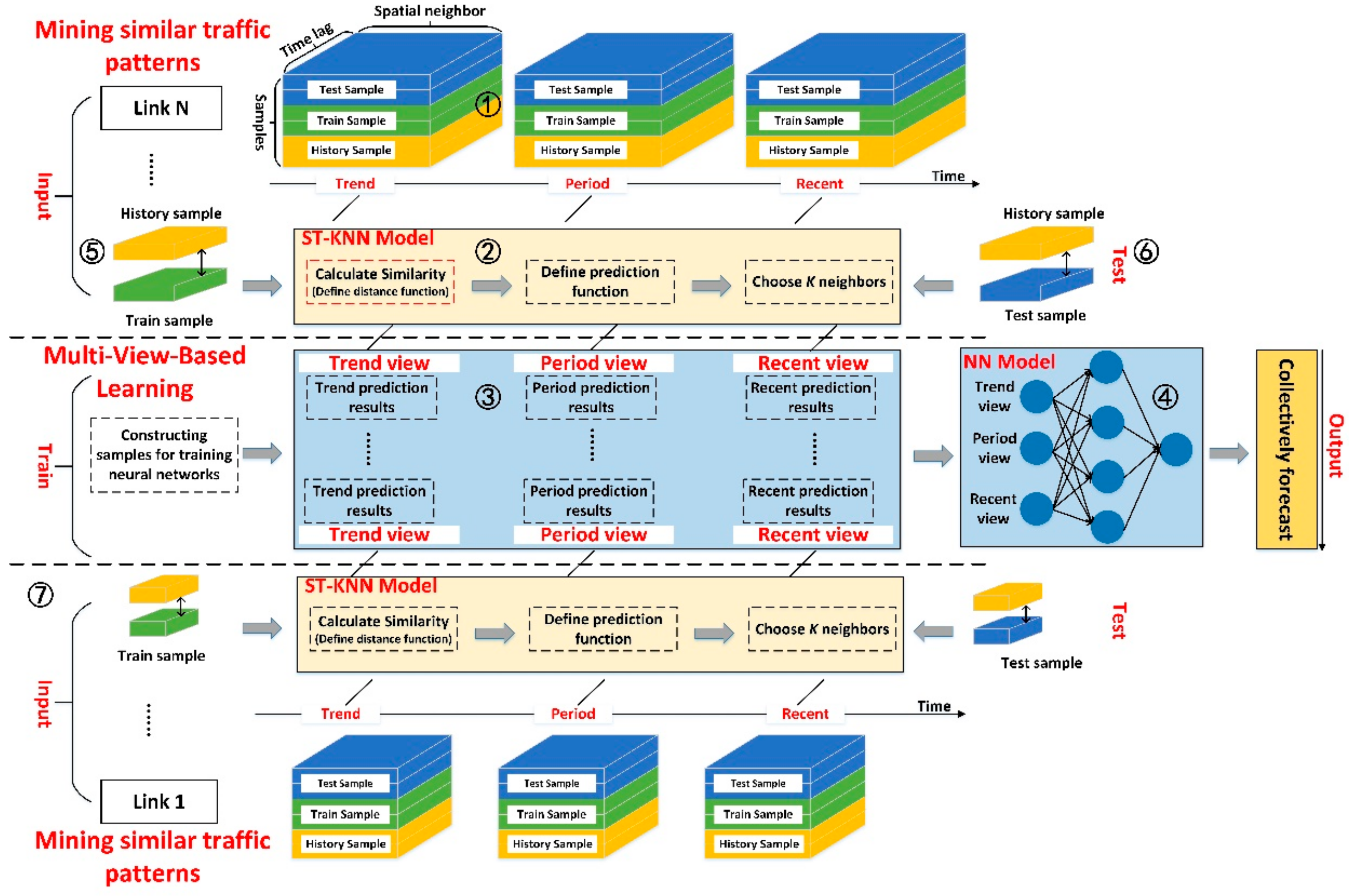
In this section, we construct the MVL-STKNN model for short-term traffic prediction for which the overall architecture is shown in Figure 1. In the model, ① represents the spatiotemporal cuboid, ② represents the modeling process of the ST-KNN model, ③ represents the sample construction of multi-view learning, ④ represents the multi-view learning process, ⑤ and ⑥ represent the candidate neighbor selection process for the ST-KNN model in training data sets and test data sets, and ⑦ represents the modeling process of different road segments. Elements ①, ②, ③, ⑤, and ⑥ are used to construct the model inputs and ④ is used for model training. The overall framework is a progressive relationship at the logical level, according to the construction of spatiotemporal cuboid and the improved ST-KNN model and the multi-view-based learning methods. The spatiotemporal cuboid is used to reorganize the original historical traffic data and it uses the stacked spatiotemporal state matrix to characterize the temporal and spatial dependence of traffic conditions. The improved ST-KNN model (the red-dashed box in ② is the improved part) exploited the constructed spatiotemporal cuboid as input to similar traffic patterns and, therefore, obtained predictions, according to the spatiotemporal closeness, periodicity, and trend views. The three predictions are used as training samples and input to the multi-view learning model for fusion. After developing the trained MVL-STKNN model, the test sample is the input to obtain predictions of traffic conditions. It should be noted that, since we consider spatial heterogeneity in the modeling process, the main difference between the modeling processes represented by ⑦ and ①–⑥ is that the dimensions of the spatiotemporal cuboids are different.
2.1. Construction of Space-Time Cuboid
In the road network, traffic conditions on road segments are space–time constrained. In the spatial dimension, traffic conditions on road segments are usually influenced by the surrounding road segments. For example, congestion on one road segment may spread to surrounding segments over time, which leads to regional congestion [37]. In our research study, the surrounding road segments refer to the road segments within the third-level topological neighbors of the predicted road segment. This type of influence has spatial heterogeneity, which means the number of surrounding road segments affected by different road segments is inconsistent. In the time dimension, due to the existence of traffic patterns, the traffic state on road segments is usually associated with historical traffic conditions and displays temporal closeness, periodicity, and trend. Therefore, in the MVL-STKNN model, the time series of historical traffic conditions are reorganized by the fusion of spatiotemporal dimension information to form the spatiotemporal closeness matrix, the period matrix, and the trend matrix, which characterizes the traffic conditions on any road segment at any time. All of the spatiotemporal state matrices are then stacked according to the time necessary to form three spatiotemporal cuboids in order to depict the spatiotemporal dependence of road segments.
By taking the structure of the spatiotemporal closeness cuboid as an example, we assume that the time series representing traffic conditions is , where and represent the start time-step and the current time-step of the time series, is the number of road segments, and is the traffic conditions of the road segment at time interval . For each road segment , the spatiotemporal closeness state matrix at time interval can be expressed as . The elements in the spatiotemporal closeness state matrix represent traffic conditions on the relevant surrounding road segments at historically recent time intervals, which is formally defined by the equation below.
where is the length of the closeness-dependent sequence. The traffic conditions of historical time intervals adjacent to the time interval are selected within the range. represents the set of spatial neighbors of road segment and each road segment has a different set of spatial neighbors. represents the number of spatial neighbors;.
In a similar way, the formal definitions of spatiotemporal periodicity matrix and spatiotemporal trend matrix are shown in the equations below.
where is the length of the period-dependent sequence and is the value set of the temporal period: . is the length of the trend-dependent sequence and is the value set of temporal trends: .
In this scenario, the is the sampling time interval of traffic conditions such as 5 min (where one day = 1440 min). is the period span and is the trend span. For example, = 1 describes daily periodicity and = 7 reveals the weekly trend.
The spatial neighbor set of the road segment is automatically obtained using cross-correlation. Considering the delay in spatiotemporal dependency between road segments, the traditional way to find spatial neighbors using correlation coefficients does not satisfy this requirement. The cross-correlation function, as a delayed version of the correlation coefficient function, measures the correlation coefficients of two time series using a specific delay [38] and is better suited to describing the spatiotemporal dependence of traffic. Assume that the traffic condition time series of two road segments are, respectively: ,. Then the cross-correlation functions at delayed are defined by the equation below.
where is the cross-correlation coefficient of time series and time series at delay . and are the mean values of and , respectively. Parameters and are the standard deviations of and , respectively. From the above definition, the cross-correlation function can be regarded as a function of time delay so that the maximum time delay value of the cross-correlation function is the average delay time of the surrounding road segments to the predicted road segment [29], which can be formally defined by Equation (7).
where is the maximum time delay value of the surrounding road segment for predicting the road segment . Given the predicted road segment and its prediction time range , only those surrounding road segments that can be accessed within the maximum time delay are considered and the road segments beyond the time delay limit are excluded.
The corresponding maximum time delay value is obtained by calculating the cross-correlation between all the surrounding road segments and the predicted road segments. Finally, all the road segments satisfying the conditions are added to the set.
After completing the construction of the spatiotemporal state matrix at all historical time intervals, we stacked three spatiotemporal state matrices in chronological order and constructed spatiotemporal closeness cuboids, periodic cuboids, and trend cuboids of road segments . Their formal definitions are shown below.
where , which ensures that the temporal closeness matrix, the period matrix, and the trend matrix can be taken simultaneously at time interval .
Finally, we divide the spatiotemporal cuboid ,, respectively, including historical spatiotemporal cuboids and a historical template library for mining similar traffic patterns in the ST-KNN model. We also divide training spatiotemporal cuboids for input to the ST-KNN model in comparison with the historical template library to obtain forecasts from each view in order to construct the training samples for multi-view learning as well as test spatiotemporal cuboids for verification of model prediction accuracy, as shown in Figure 1. We take as the total days of the time series of traffic conditions, the number of historical days as , the number of training days as , and the number of test days as . Then , where is the number of days that the sample cannot be taken simultaneously. The number of historical samples is , the number of training samples is , and the number of test samples is . Taking the partition of the temporal closeness cuboid as an example, the historical spatiotemporal closeness cuboid , the training spatiotemporal closeness cuboid , and the test spatiotemporal closeness cuboid can be defined by the formulas below.
The same division method can be used to obtain the historical spatiotemporal period cuboid , the training spatiotemporal period cuboid , the test spatiotemporal period cuboid , the historical spatiotemporal trend cuboid , the training spatiotemporal trend cuboid , and the test spatiotemporal trend cuboid .
2.2. ST-KNN Model
The basic principle of the ST-KNN model is to compare the distance between the spatiotemporal state space, select closest historical spatiotemporal state matrices, and use predictive functions to integrate the traffic conditions at the next time interval for the target road segment to obtain a final predicted value. In Section 2.1, we obtained the spatiotemporal state matrix of the three views. Therefore, the key here is how to define the distance function and the prediction function.
When defining the distance function, different weightings need to be introduced to describe the influence of traffic conditions at different time intervals and different spatial neighbors on predicting road segments in the spatiotemporal state matrix. In the traditional method, too many parameters are often introduced when setting the weightings, which makes it difficult to adjust the parameters in the modeling process and inhibits global optimal prediction results. Considering that the cross-correlation function characterizes the correlation between the surrounding road segments and the predicted road segments without additional parameters, we use the cross-correlation coefficient to represent the spatial weighting value for the predicted road segment in the spatial dimension, which becomes more closely related to the predicted road segment with greater weighting. In the time dimension, the time weight is assigned according to the linear distribution of time. The closer it is to the predicted time, the greater the assigned weighting. Taking the spatiotemporal closeness matrix as an example, the weighting allocation method is shown below.
where is the cross-correlation coefficient between the spatial neighborhood (whose road segment is ) and the time series of the predicted road segment . By introducing space–time weightings into the original spatiotemporal closeness matrices, the spatiotemporal neighboring weight matrices and at time interval and at a historical time interval are represented as Equations (15) and (16).
It should be noted that belongs to the historical sample library of the ST-KNN model. Therefore, its value range is limited to the set . Furthermore, is used for comparing with to obtain the candidate neighbors. Therefore, its value range is . By calculating the distance between the spatiotemporal closeness matrix at time interval and the historical spatiotemporal closeness matrix, it can be used to select candidate neighbors. The formula is below.
where represents the trace of the matrix. The distance function of the spatiotemporal periodic and trend matrix can be defined in a similar way.
When defining the predictive function, we used the same strategy as in Reference [27] and utilized the Gaussian function to assign different weightings to the selected candidate neighbors to obtain the predicted value for the target road segment . Taking the spatiotemporal closeness cuboid as an example, the form is defined below.
where represents the prediction value of road segment at time interval and represents the traffic condition of candidate neighbors at the next time interval. represents the weighting of the candidate neighbors of the prediction road segment . Its form is defined below.
where is the distance between the candidate neighbor and the predicted road segment ; is the spatiotemporal parameter. Using the same prediction function, we can obtain the predicted values and of the periodic view and the trend view of the road segment at time interval respectively.
2.3. Multi-View-Based Learning
The basic principle of the multi-view learning model is to build a supervised learning method, which takes the prediction results of the spatiotemporal closeness, periodicity, and trend views as inputs to neural network models. The real values for traffic conditions as outputs.
The process of training the MVL-STKNN model is shown in Algorithm 1. First, we use the ST-KNN model to obtain predicted values for the training spatiotemporal closeness matrix , the training spatiotemporal periodic matrix , and the training spatiotemporal trend matrix for each spatiotemporal state matrix in training spatiotemporal cuboids (lines 4–6 lines in Algorithm 1). Afterward, the predictive values of the three views are used as the feature vector and the true values are used as label values to construct the training sample (line 7). Finally, the training samples are input to the neural network model for supervised learning (line 9) and the MVL-STKNN model can be obtained (line 10).
| Algorithm 1: Training of MVL-STKNN |
| Input: Near spatiotemporal cuboids: ; |
| Periodic spatiotemporal cuboid: ; |
| Trend spatiotemporal cuboid: ; |
| Lengths of closeness, period, trend: ,,; |
| Number of candidate neighbors: ; |
| Parameter of Gaussian function: . |
| Output: MVL-STKNN model . |
| // construct training instances |
| 1 |
| 2 For all time interval in the training spatiotemporal cuboids |
| 3 // |
| 4 = ST-KNN() // |
| 5 = ST-KNN() // |
| 6 = ST-KNN() // |
| 7 Put a training instance into |
| 8 End for |
| // Training the model |
| 9 // Neural network training |
| 10 Output the learned MVL-STKNN model |
After obtaining the trained MVL-STKNN model , we can predict all samples of the test spatiotemporal cuboid. The prediction process is shown in Algorithm 2. First, the spatiotemporal closeness matrix , spatiotemporal periodic matrix , and spatiotemporal trend matrix in all the test spatiotemporal cuboids are input to the ST-KNN model to obtain the predicted values of the three views (lines 3–5 in Algorithm 2). Note that the range of the spatiotemporal state matrix is different from the training process. Additionally, the predicted values obtained by the ST-KNN model are input to the trained MVL-STKNN model and we get the final prediction value of the road segment at the next time interval (line 6). Finally, the predicted values for all the test samples are saved to set for evaluating the accuracy of the MVL-STKNN model (line 7).
| Algorithm 2: Prediction of MVL-STKNN |
| Input: Near spatiotemporal cuboids: ; |
| Periodic spatiotemporal cuboid: ; |
| Trend spatiotemporal cuboid: ; |
| Lengths of closeness, period, trend: ,,; |
| Number of candidate neighbors: ; |
| Parameter of Gaussian function: . |
| Output: Set of test sample predictions: . |
| 1 For all time interval in the test spatiotemporal cuboids |
| 2 // |
| 3 = ST-KNN() // |
| 4 = ST-KNN() // |
| 5 = ST-KNN() // |
| 6 // Obtain the predicted values |
| 7 Put into // Save the predicted values into set |
| 8 End for |
| 9 Return the set of predictions |
3. Performance Evaluation
In this section, we use floating car-speed data collected for the Beijing road network and the California Freeway and Expressway systems to evaluate the proposed MVL-STKNN model. First, we pre-process the raw traffic data and demonstrate its heterogeneous attributes. Afterward, in the Beijing data set, we adjust the parameters of the MVL-STKNN model to obtain a set of optimal parameter combination values. On this basis, we compare existing baseline methods to verify the efficiency of the proposed model. At the same time, the generalizability of the MVL-STKNN model was tested by further comparing the accuracy of different traffic prediction models using the Caltrans Performance Measurement System (PeMS) datasets. Finally, taking the Beijing dataset as an example, the impact of each component on the overall prediction accuracy of the model is explored including the time–space weighting and spatiotemporal dependence components proposed in this study.
3.1. Data Preparation
3.1.1. Data Sources
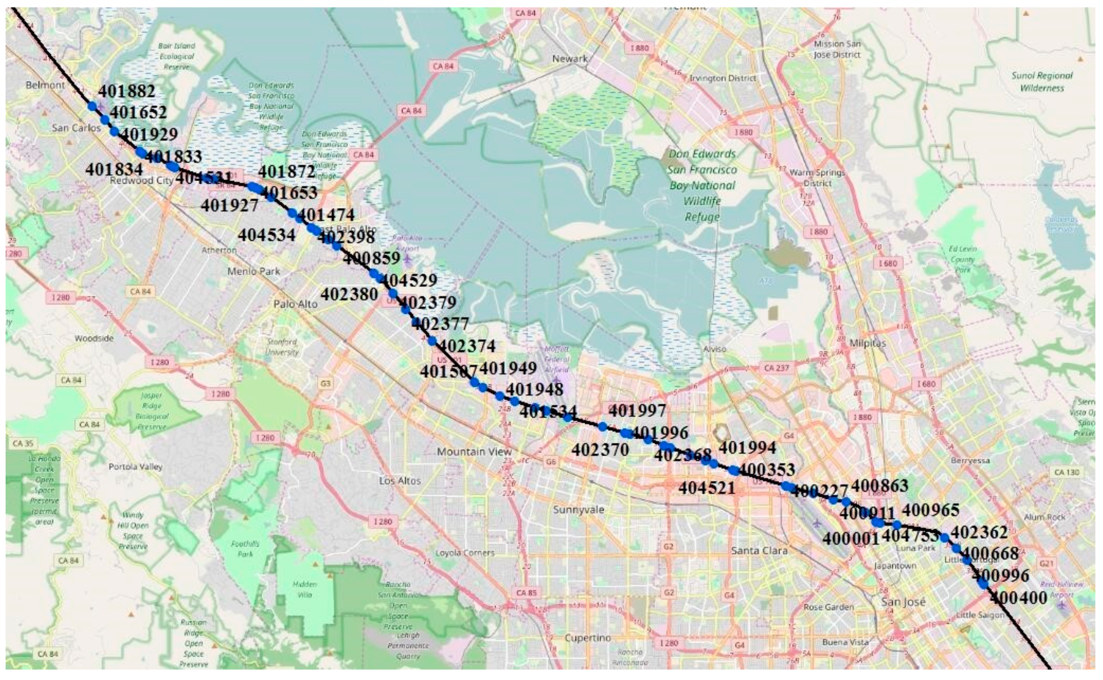
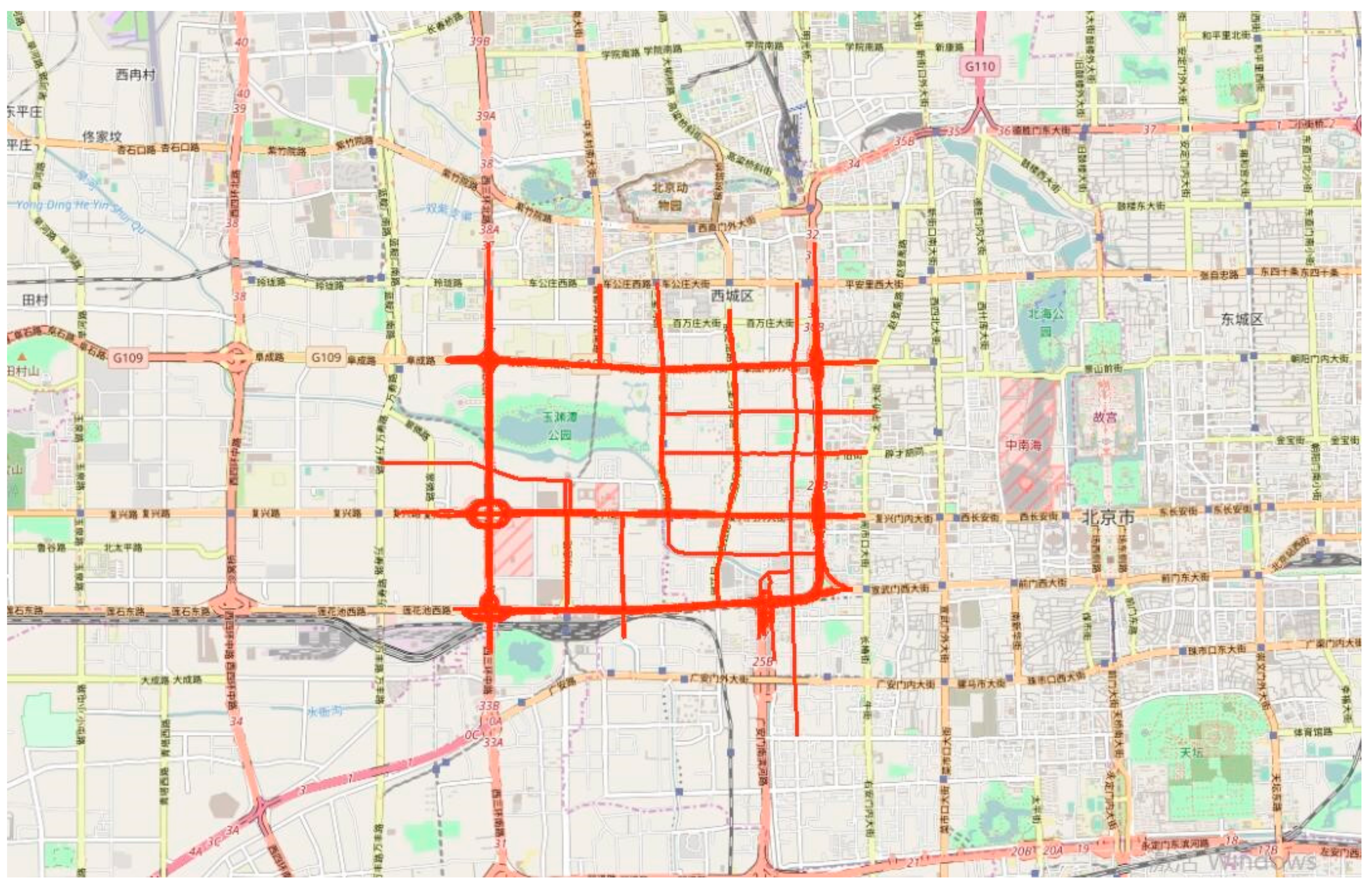
We used floating car-speed data collected from the Beijing road network and the California Freeway and Expressway systems to evaluate the performance of the models by predicting the vehicular speed of the road segment. These data points are widely applied in the field of transportation [14,23,39,40]. Among these, PeMS continuously collects real traffic data from more than 8100 locations on the California Freeway and Expressway systems. These data are integrated into multiple time intervals and are freely available on the network [41]. PeMS travel speed data were downloaded for 59 consecutive locations on the US Route 101 and the data distribution is shown in Figure 2. The data were collected at 5-min intervals for 60 days (15 August 2016 to 14 October 2016), which was shown in Table 1. The Beijing dataset comes from the driving track of a GPS-equipped floating car by uploading driving-related information to the server at one-minute intervals, including travel time, direction, and speed. The time period is from 1 March 2012 to 30 April 2012, which is shown in Table 1. We integrated the data into 5-min intervals, calculate the average speed of each road segment, and finally selected 30 representative road segments for subsequent experiments. The data distribution is shown in Figure 3. In both data sets, data from the last five days were used as test data to construct the test spatiotemporal cuboids and five days were used to construct training spatiotemporal cuboids.
3.1.2. Data Processing
Due to equipment failure and other factors, some data were missing from the original traffic-speed data sets. Considering the spatiotemporal characteristics of traffic data, we used the existing spatiotemporal interpolation algorithm to fill in the missing data in order to better reconstruct the original traffic conditions [42]. The basic principle is to consider the missing data pattern in the interpolation process and use coarse-grained interpolation to obtain partial reconstruction results in order to eliminate the effect of missing continuous block data on the subsequent interpolation process. On this basis, considering the spatiotemporal heterogeneity, fine-grained interpolation was applied to the spatial and temporal dimensions. Finally, the unbiased estimation values of the missing data were obtained by integrating the interpolation results of the spatiotemporal dimensions in a nonlinear way. Considering that travel speeds on different types of road segments vary greatly across the road network, we normalized the original traffic data and used the ratio of the average speed to a maximum speed limit on each road segment to represent the traffic conditions of road segments. This is expressed in Formula (20).
In this study, is the normalized speed of the road segment at time interval , is the average speed of the road segment and is the speed limit of the road segment.
3.2. Evaluation Metrics
Similarly, with regard to other traffic prediction studies [9,10,26,27], the present study uses the mean absolute percentage error (MAPE) as a measure of performance, which reflects the percentage difference between predicted and actual traffic conditions. The prediction accuracy of different models is depicted by averaging the percentage error of traffic conditions for all road segments during the test time interval. A smaller MAPE value indicates higher accuracy of the prediction model. The formal definition is below.
where is the start time interval of the test data and and are the actual vehicular speed and the predicted vehicular speed at the next time step of the predicted road segment at the current time step. After dividing the test data set for the original traffic time series, the equations and are satisfied.
3.3. Variable Estimation
The MVL-STKNN hyper parameters include parameter , the number of candidate neighbors , the length of the closeness-dependent sequence , the length of the periodic-dependent sequence , and the length of the trend-dependent sequence . We set up a reasonable range of values for each parameter in order to find the combination of parameter values that achieves the lowest MAPE where , , ,, and. During this estimation process, the parameters were adjusted in a progressive manner. First, and were determined to obtain the optimal ST-KNN model. On this basis, the effect of temporally dependent sequence length on model accuracy was tested to determine the values of , , and .
3.3.1. Calibrating the Parameters of ST-KNN Model
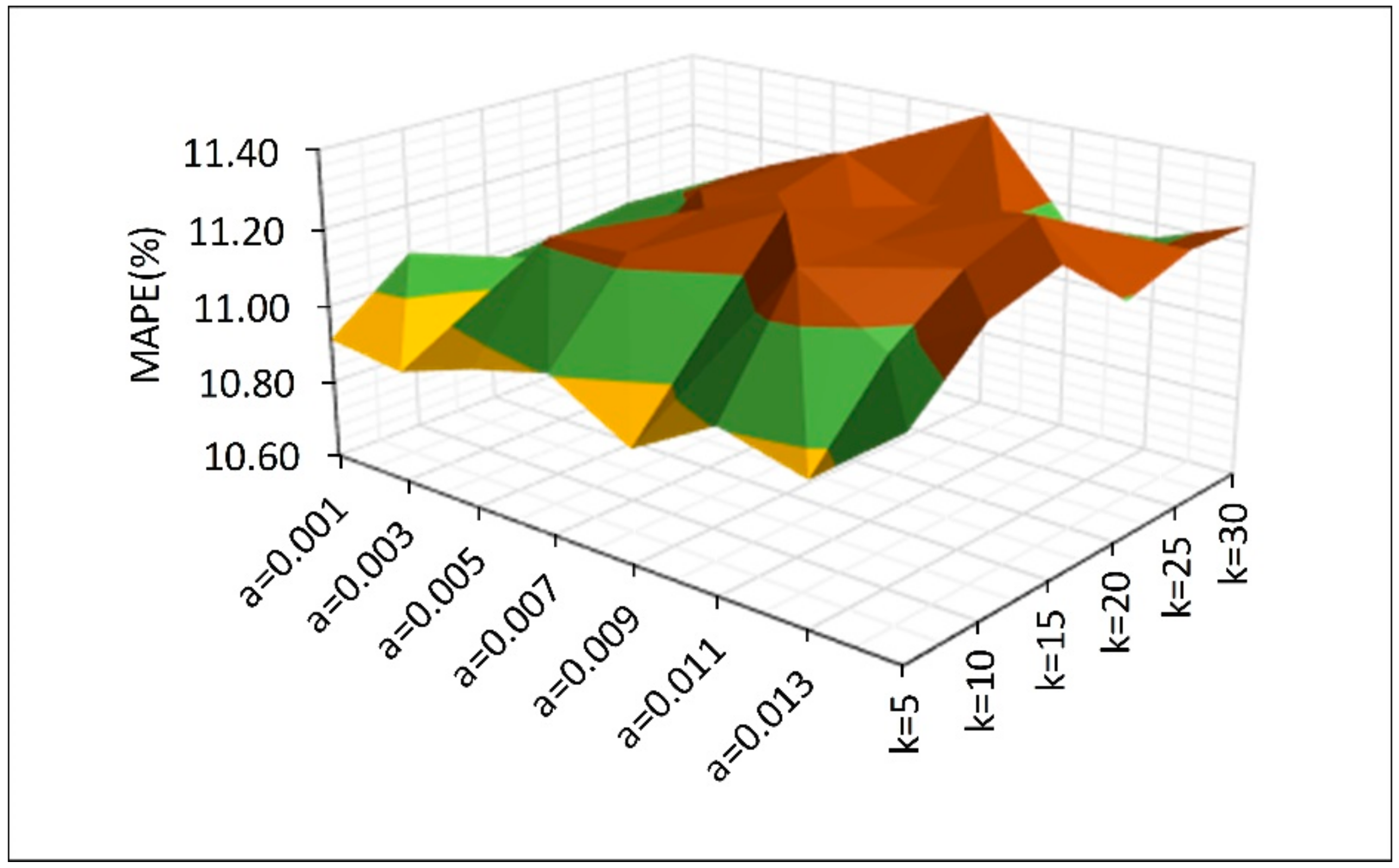
Figure 4 shows the effect of the combined values of parameters and on the prediction accuracy of the model. We fixed , , and while varying the values of parameters and , which is shown in Figure 4. It can be seen that the MVL-STKNN model has the smallest MAPE value when and . MAPE shows a small overall change, which indicates that the values of parameters and have little influence on the overall prediction accuracy of the MVL-STKNN model.
3.3.2. Calibrating the Temporally Dependent Parameters
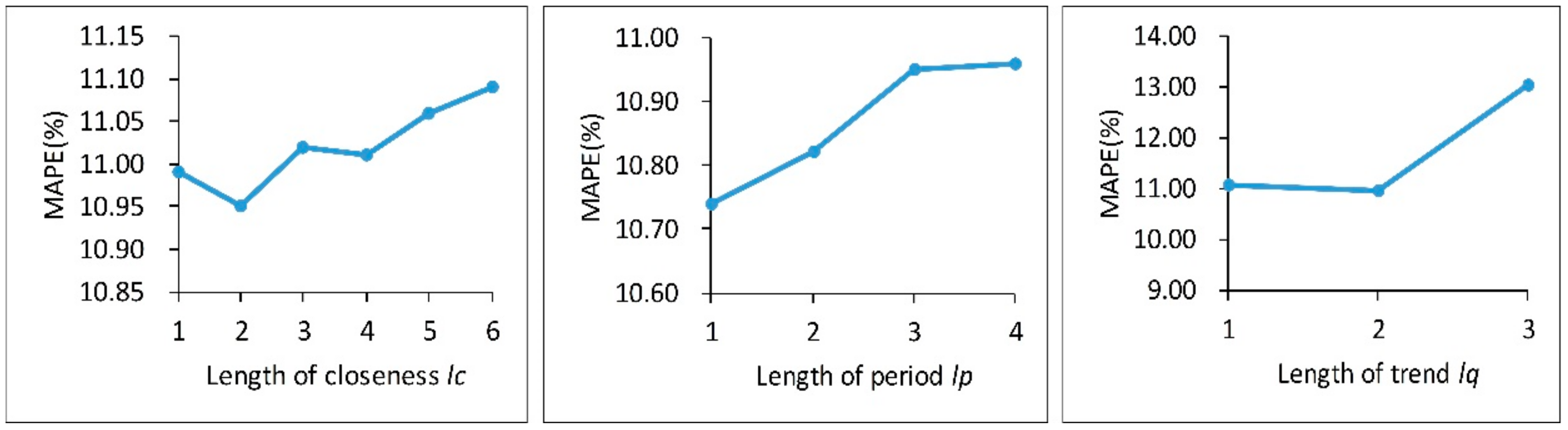
Furthermore, we verified the impacts of temporally dependent parameters on model performance, which is shown in Figure 5. First, we fixed , , and varied the value of the temporal closeness parameter to test its effect on prediction accuracy. As shown in Figure 5a, by changing , the prediction accuracy first increased and then decreased. The lowest MAPE value was recorded for . Afterward, we fixed , , and varied the value of the temporal period parameter . The resulting prediction accuracies are shown in Figure 5b. The MVL-STKNN model has the highest prediction accuracy when . As increases, prediction accuracy gradually decreases. The results show that short-range periods are helpful for prediction models while long-range periods are difficult to model. Finally, we fixed , , and varied the time trend parameter . As shown in Figure 5c, the model has a nearly equal prediction performance when or , which indicates that the short-range trend is easier to capture. When , the value of MAPE rose sharply. The reason is that the dynamic changes in traffic conditions obscure the long-range trend, which affects the prediction accuracy of the model.
Through the above parameter-debugging process, the parameter-calibration results of the MVL-STKNN model are shown in Table 2.
3.4. Test of Spatial Heterogeneity
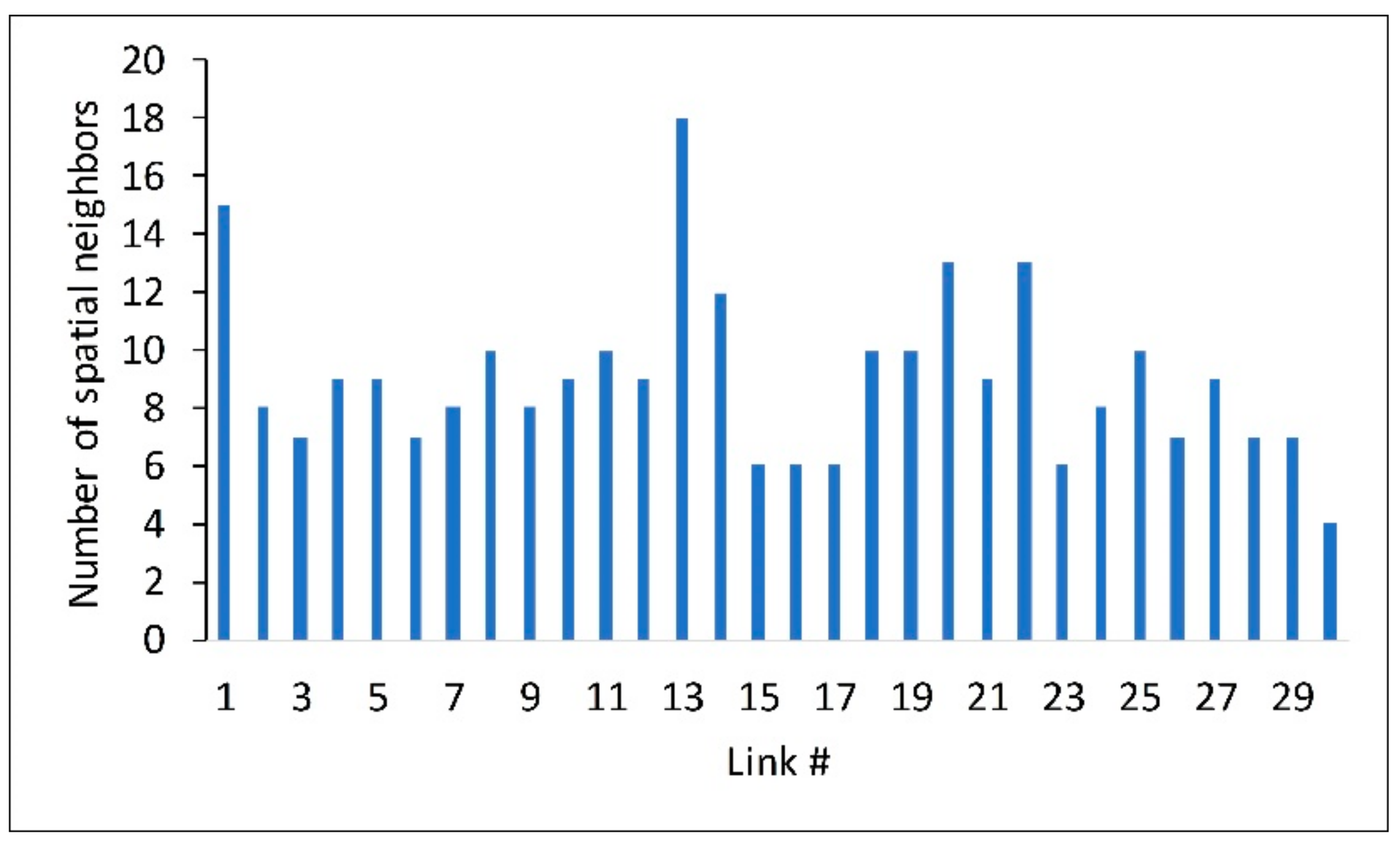
After completing the data preprocessing, we tested the heterogeneous nature of traffic. Taking 30 road segments in Beijing as an example, we used cross-correlation to automatically determine the spatial neighbors of each road segment, according to the selection strategy of spatial neighbors. The result is shown in Figure 6. The abscissa represents the IDs of the road segments and the ordinate represents the number of spatial neighbors of the road segments. For example, Link 1 has 15 spatial neighbors and Link 2 has eight spatial neighbors. It can be observed that the number of spatial neighbors of different road segments is inconsistent. The above results show that the set of spatial neighbors and the number of spatial neighbors differ for each road segment, which reflects the obvious heterogeneity of urban road traffic. Therefore, when constructing the spatiotemporal state matrix, previous studies used global fixed spatiotemporal dimensions to represent traffic conditions, which cannot reflect the heterogeneity of traffic conditions on the road network. It also confirms that the selection strategy of adaptive spatial neighbor adopted in this research study is reasonable.
3.5. Accuracy Comparison
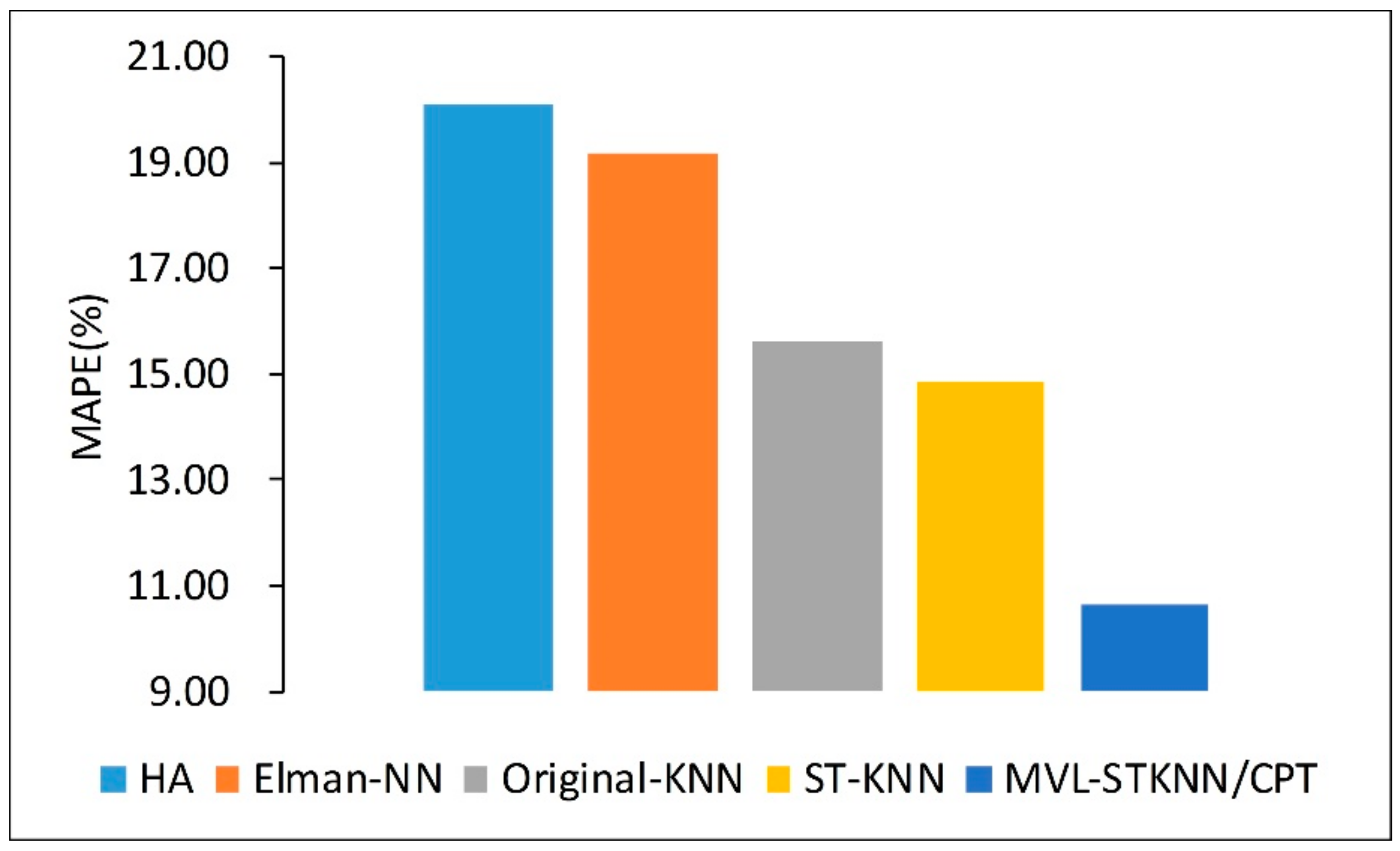
In order to verify the efficiency of the proposed MVL-STKNN model, we compared it with four existing traffic predicting models in Beijing and PeMS data sets, which are comprised of the historical average model (HA), the Elman neural network (Elman-NN), the KNN model (Original-KNN), and the spatiotemporal KNN model (ST-KNN). Of these, the HA model uses the average value of the historical time window as the prediction value of traffic condition at the next time interval. The Elman-NN model is extended to short-term traffic prediction by introducing delay operators into the model to adapt traffic time-varying features [43]. The Original-KNN model is an instance-based nonparametric supervised learning algorithm that heuristically compares the similarity of historical traffic time series with the current observed time series. Many researchers have successfully applied the KNN model to short-term traffic prediction [25,44,45]. Based on the Original-KNN model, the ST-KNN model is formed by considering the spatiotemporal relationships among multiple road segments in the road network.
Figure 7 shows the prediction accuracy of the four models when using the Beijing dataset. It can be seen that because the HA, the Elman-NN, and the Original-KNN models consider traffic forecasting as a time series modeling problem, they ignore the influence of spatial factors on the predicted road segments. Therefore, their predictive performances are worse than those of the ST-KNN model and the proposed MVL-STKNN model. The ST-KNN model introduces the spatiotemporal closeness matrix rather than the traditional time series to characterize traffic conditions and constructs the distance function and prediction function using the Gaussian function to improve the predictive performance of the model. However, in the modeling process, the spatiotemporal dependence relationship is not fully characterized. For example, in the spatial dimension, the heterogeneity of road network traffic is not considered, which results in a globally fixed dimension of its spatiotemporal adjacency matrix. In the temporal dimension, the influence of temporal periodicity and trend on the prediction of road segment traffic conditions is ignored. In addition, when the distance function is constructed, too many parameters are artificially introduced, which exacerbates the difficulty of the parameter adjustment. Consequently, the predictive accuracy of the model is significantly lower than the method proposed here. In the MVL-STKNN model, the improved ST-KNN model is first introduced by using space-time weighting rather than Gaussian weighting. On this basis, the spatiotemporal dependencies are comprehensively considered and three spatiotemporal views are constructed (spatiotemporal closeness, periodic, and trend matrices) to characterize the traffic conditions. Finally, short-term traffic prediction is achieved by using a multi-view learning method. It can be seen from Figure 7 that the MVL-STKNN model reduces the MAPE between 28.24% and 46.86% compared with the existing methods, which indicates that the proposed method solves the problems existing in the baseline method.
Since urban road networks and freeway exhibit different road network topological structures and have large differences in traffic patterns, we further validated the model’s performance on PeMS datasets. The experimental results are shown in Figure 8. Overall, the accuracy trend of the model was similar to that of the Beijing dataset, but the predictive accuracy was more extensive. This is attributed to higher data quality. The PeMS data set is relatively complete and, because the data collection area is an expressway, the traffic pattern is relatively simple when compared with an urban road network. The change trend is small, which makes it easier to capture the regular traffic pattern. As can be seen from Figure 8, the MVL-STKNN model reduces the MAPE between 53.80% and 90.29%. When compared with the existing methods, this further demonstrates the effectiveness of the proposed method and its satisfactory generalization.
3.6. Impact of Space-Time Weighting Matrix
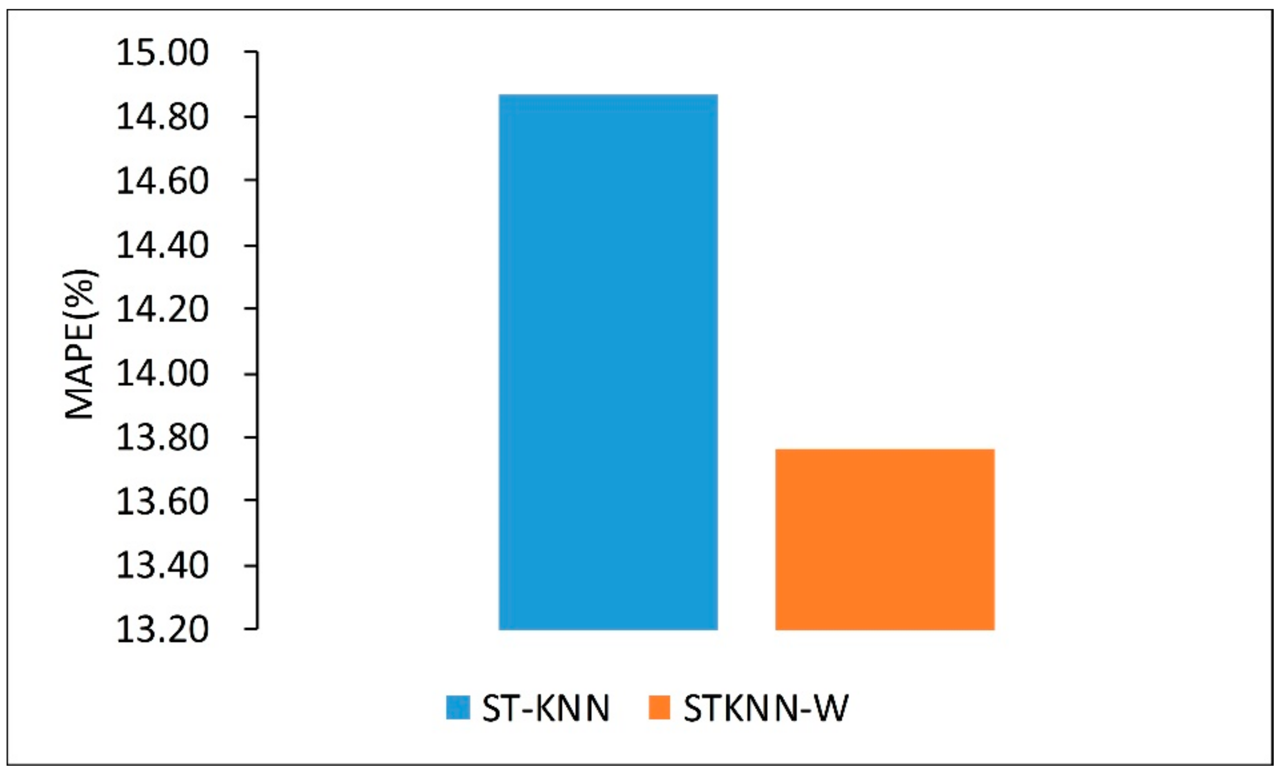
Based on the existing ST-KNN model, we use space–time weighting allocation instead of the traditional Gaussian function allocation method to construct the STKNN-W model. The experimental results in Figure 9 clearly demonstrate that the proposed method achieves superior performance, which is attributed to the MVL-STKNN model by employing the ST-KNN model to mine similar traffic patterns and to derive predictions for the spatiotemporal closeness, periodic, and trend views. In the training process, these three sets of predictions are then used to construct training samples for multi-view learning. During testing, the parameters trained through multi-view learning are used to integrate the three views to give predicted values for traffic conditions on the road segments. Therefore, the performance of the ST-KNN model will have a certain impact on the overall prediction results. In the ST-KNN model, the key is how to construct a suitable distance function to select the candidate neighbors. The existing ST-KNN constructs the distance function using a Gaussian function to allocate weightings in the time and space dimensions, respectively. Compared with Euclidean distance and correlation distance, the predictive accuracy of the model is somewhat improved [27]. However, the Gaussian weight function requires the introduction of additional parameters, which exacerbates the difficulty of parameter calibration. In contrast, the proposed weight allocation method does not require additional parameters. Moreover, the influence of traffic conditions with different time intervals and different spatial neighbors on the predicted road segments can be mined from the data itself, which achieves higher prediction accuracy.
3.7. Impact of Spatial and Temporal Dependencies
In this section, we further discuss the impacts of spatial and temporal dependencies on the overall results.
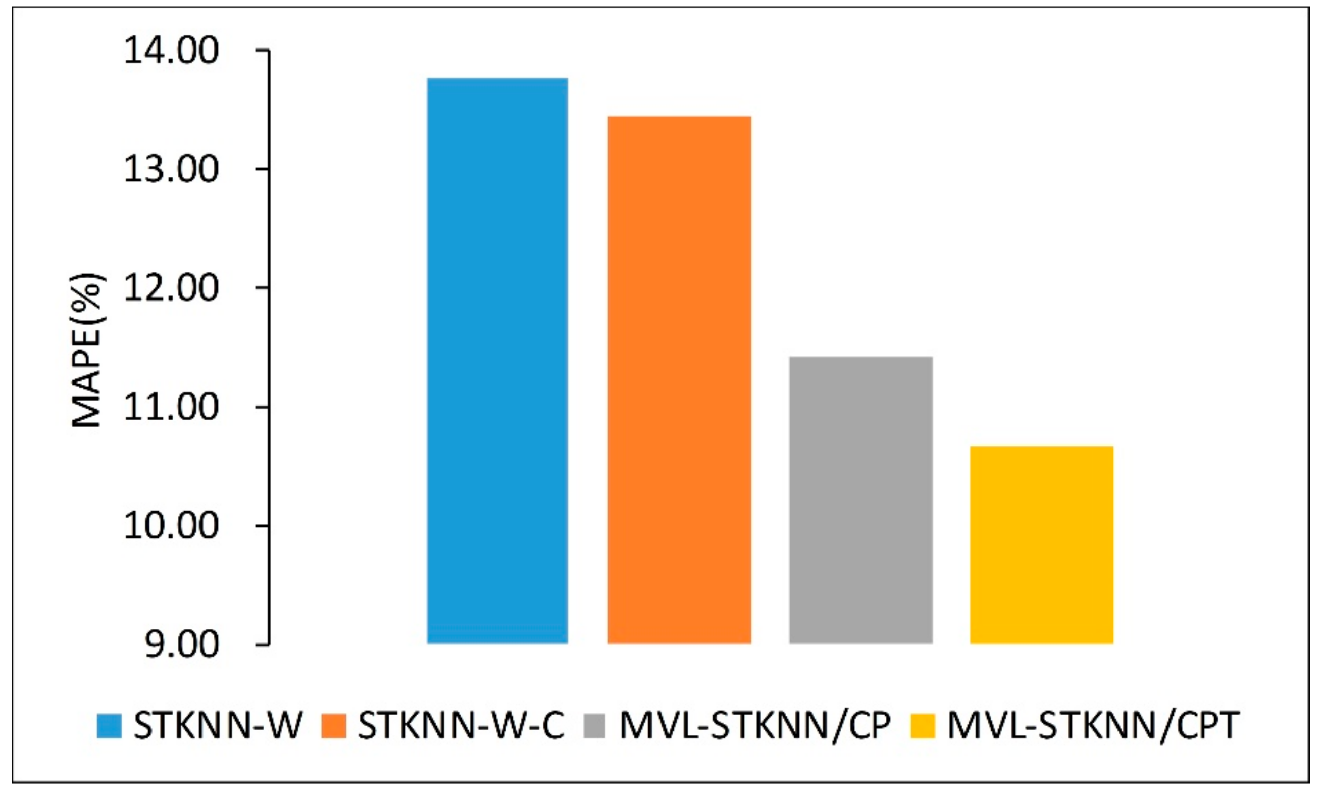
First, we test the effect of spatiotemporal closeness on predictive accuracy. Considering that the existing ST-KNN and STKNN-W models use the globally fixed spatiotemporal closeness matrix to characterize traffic conditions, they cannot cope with the heterogeneous nature of traffic conditions. Therefore, based on the STKNN-W model, we hold other variables fixed and automatically select the spatial neighbors for each road segment using cross-correlation so that the spatial neighbors of each road segment are different (see Figure 4). Afterward, the STKNN-W-C model is constructed using the adaptive spatiotemporal closeness matrix rather than the traditional globally fixed spatiotemporal closeness matrix. As can be seen from Figure 10, the STKNN-W-C model is more accurate than STKNN-W, which confirms the validity of the adaptive spatiotemporal closeness matrix.
Second, on the basis of the STKNN-W-C model, we further introduce temporal periodicity, which is combined with an adaptive spatial neighbor to form a spatiotemporal periodic matrix to represent traffic conditions from another view. Since the entire model contains two views, it can constitute a multi-view learning method known as MVL-STKNN/CP, which considers both spatiotemporal closeness and period. The training and prediction process is similar to that shown in Algorithms 1 and 2 except that the spatiotemporal trend view is not included. As shown in Figure 10, the performance of the MVL-STKNN/CP model is significantly improved, which demonstrates the usefulness of spatiotemporal periodicity in the modeling process. Multi-view learning has the potential to accurately predict short-term traffic.
Finally, on the basis of the MVL-STKNN/CP model, we further introduce the spatiotemporal trend matrix to form a complete MVL-STKNN/CPT model. Based on the introduction of space–time weightings, we simultaneously consider spatiotemporal closeness, the period, and the trend to form a multi-view learning method. It can be seen that the predictive accuracy of MVL-STKNN/CP is further improved. This demonstrates the validity of the spatiotemporal trend.
In addition, from comparing the improved models, comprising STKNN-W, STKNN-W-C, MVL-STKNN/CP, and MVL-STKNN/CPT, the introduction of periodicity induces the largest improvement in prediction accuracy, which induces the smallest improvement. Since the trend has a greater time span than periodicity, it is more difficult to capture the changing characteristics of traffic patterns.
4. Discussion
Accurate and robust short-term vehicular speed forecasting is a critical issue in superior transportation systems and traffic related applications. The existing ST-KNN model uses distance functions and correlation coefficients to identify spatial neighbors and measures the temporal interaction by only considering the temporal closeness of traffic, which means that existing ST-KNNs cannot fully reflect the essential features of road traffic. We address the shortcomings of such models by introducing an improved spatiotemporal KNN model integrated with multi-view learning. The proposed model greatly improves the performance of short-term traffic forecasting. However, there are still some issues that require further investigation.
Considering the spatial heterogeneity of city traffic, traffic patterns of different road segments show significant differences [46,47], which is reflected in different model structures including different spatial neighbors and spatiotemporal parameters. In the MVL-STKNN model, we have constructed an adaptive spatial neighbor for each road segment. However, in order to simplify the model (for example, in the modeling process, there is no need to adjust the parameters of each road segment), we adopt the mechanism of sharing parameters, which need further refinement in future work.
Yet, we consider the temporal proximity, periodicity, and trend to characterize the temporal non-stationarity of different road segments in the MVL-STKNN model. However, from the perspective of the more fine-grained variation characteristics of temporal non-stationarity, different road segments may have different fluctuation patterns in different time periods such as morning and evening peaks. Therefore, a very promising approach is to identify the traffic pattern of the entire road network through a clustering algorithm and then divide the time period for each traffic pattern. Next, the MVL-STKNN model is constructed for each time period in each cluster to further improve the accuracy and robustness of short-term traffic prediction.
Finally, we only validated the MVL-STKNN model with a small dataset. For example, 30 representative road segments and five days of data in the Beijing dataset were selected to test the performance of the proposed model. As mentioned above, different road segments show different traffic patterns at different time periods in order to use more road segments and a longer prediction period to comprehensively evaluate the accuracy and robustness of the MVL-STKNN model.
5. Conclusions
In this paper, we propose the MVL-STKNN model for short-term vehicular speed prediction. First, considering the heterogeneous nature of traffic, different road segments have different numbers of spatial neighbors. Therefore, we use cross-correlation to automatically determine the spatial neighbors of each road segment, which overcame the problem that existing methods can not automatically capture spatial information. Afterward, we consider temporal closeness, periodicity, and trend. This is further combined with an adaptive spatial neighbor to form three characterizations of traffic conditions including matrices for spatiotemporal closeness, period, and trend, which overcomes the problem that existing methods only use a global, fixed spatiotemporal closeness matrix to describe the traffic condition. Second, we introduce space–time weighting to improve the distance function in the ST-KNN model, which is then used to mine similar traffic patterns and obtain prediction results for the three spatiotemporal views, respectively. Finally, a multi-view learning method based on the neural network model is constructed from these three predicted spatiotemporal views with different weightings allocated to these views to obtain prediction values for traffic conditions.
In the experimental section, we employ two widely used traffic data sets comprised of floating car-speed data collected from the Beijing road network and from the California Freeway and Expressway systems to verify the efficiency of the proposed model. We first conducted a comparison with four existing baseline methods including HA, Elman-NN, KNN, and ST-KNN models. Compared the existing methods, the MVL-STKNN model decreases the MAPE index anywhere from 28.24% to 46.86% in the Beijing dataset and anywhere from 53.80% to 90.29% in the PeMS dataset. This demonstrates the efficiency of the multi-view learning method. Second, we further explore the influence of the components of the MVL-STKNN model on predictive accuracy. For the space–time weighting matrix, the problem of parameter calibration of the existing ST-KNN model is solved by using space–time weighting instead of Gaussian weighting in the distance function. For spatiotemporal dependencies, the introduction of the adaptive spatial neighbor, temporal periodicity, and the trend in road traffic significantly improves the performance of short-term traffic forecasting, which demonstrates that the multi-view learning approach merits further attention in traffic-related data mining under such a dynamic and data-intensive environment. This needs to be considered with regard to the spatial correlation and heterogeneity as well as temporal closeness, periodicity, and trend in road traffic.
For the direction of future work, the following problems need to be investigated: (1) Further validation of the proposed model using more road segments and longer prediction periods, (2) comprehensive comparison of other spatiotemporal modeling methods such as ST-ARIMA and ST-ANN, and (3) incorporating external factors into the modelling process such as weather conditions and traffic accidents, and integrating these into the MVL-STKNN to achieve a more robust model that would further improve short-term traffic forecasting.
Author Contributions
S.C. and F.L. conceived the idea for the research and wrote the paper. S.C. implemented the ST-2SMR model and carried out the experimental validation. F.L. interpreted the results. P.P. and S.W. made important comments and suggestions for this paper.
Funding
This research was funded by the Key Research Program of the Chinese Academy of Sciences, grant number ZDRW-ZS-2016-6-3 and the State Key Research Development Program of China, grant number 2016YFB0502104. Their supports are gratefully acknowledged.
Acknowledgments
We also thank the anonymous referees for their helpful comments and suggestions.
Conflicts of Interest
The authors declare no conflict of interest.
References
- Xia, J.; Chen, M.; Huang, W. A multistep corridor travel-time prediction method using presence-type vehicle detector data. J. Intell. Transp. Syst. Technol. Plan. Oper. 2011, 15, 104–113. [Google Scholar] [CrossRef]
- Vlahogianni, E.I.; Golias, J.C.; Karlaftis, M.G. Short-term traffic forecasting: Overview of objectives and methods. Transp. Rev. 2004, 24, 533–557. [Google Scholar] [CrossRef]
- Van Lint, J.W.C.; Van Hinsbergen, C. Short-term traffic and travel time prediction models. Artif. Intell. Appl. to Crit. Transp. Issues 2012, 22, 22–41. [Google Scholar]
- Levin, M.; Tsao, Y.-D. On forecasting freeway occupancies and volumes. Transp. Res. Rec. 1980, 773, 47–49. [Google Scholar]
- Guo, J.; Williams, B.M. Real-Time Short-Term Traffic Speed Level Forecasting and Uncertainty Quantification Using Layered Kalman Filters. Transp. Res. Rec. J. Transp. Res. Board 2010, 2175, 28–37. [Google Scholar] [CrossRef]
- Guo, J.; Huang, W.; Williams, B.M. Adaptive Kalman filter approach for stochastic short-term traffic flow rate prediction and uncertainty quantification. Transp. Res. Part C Emerg. Technol. 2014, 43, 50–64. [Google Scholar] [CrossRef]
- Smith, B.L.; Williams, B.M.; Keith Oswald, R. Comparison of parametric and nonparametric models for traffic flow forecasting. Transp. Res. Part C 2002, 10, 303–321. [Google Scholar] [CrossRef]
- Clark, S. Traffic Prediction Using Multivariate Nonparametric Regression. J. Transp. Eng. 2003, 129, 161–168. [Google Scholar] [CrossRef]
- Zheng, Z.; Su, D. Short-term traffic volume forecasting: A k-nearest neighbor approach enhanced by constrained linearly sewing principle component algorithm. Transp. Res. Part C Emerg. Technol. 2014, 43, 143–157. [Google Scholar] [CrossRef] [Green Version]
- Habtemichael, F.G.; Cetin, M. Short-term traffic flow rate forecasting based on identifying similar traffic patterns. Transp. Res. Part C Emerg. Technol. 2016, 66, 61–78. [Google Scholar] [CrossRef]
- Khosravi, A.; Mazloumi, E.; Nahavandi, S.; Creighton, D.; Van Lint, J.W.C. A genetic algorithm-based method for improving quality of travel time prediction intervals. Transp. Res. Part C Emerg. Technol. 2011, 19, 1364–1376. [Google Scholar] [CrossRef]
- Park, J.; Li, D.; Murphey, Y.L.; Kristinsson, J.; McGee, R.; Kuang, M.; Phillips, T. Real time vehicle speed prediction using a Neural Network Traffic Model. In Proceedings of the International Joint Conference on Neural Networks, San Jose, CA, USA, 31 July–5 August 2011; pp. 2991–2996. [Google Scholar] [CrossRef]
- Koesdwiady, A.; Soua, R.; Karray, F. Improving Traffic Flow Prediction with Weather Information in Connected Cars: A Deep Learning Approach. IEEE Trans. Veh. Technol. 2016, 65, 9508–9517. [Google Scholar] [CrossRef]
- Ma, X.; Dai, Z.; He, Z.; Ma, J.; Wang, Y.Y.; Wang, Y.Y. Learning traffic as images: A deep convolutional neural network for large-scale transportation network speed prediction. Sensors 2017, 17, 1–16. [Google Scholar] [CrossRef] [PubMed]
- Vlahogianni, E.I.; Karlaftis, M.G.; Golias, J.C. Spatio-temporal short-term urban traffic volume forecasting using genetically optimized modular networks. Comput. Civ. Infrastruct. Eng. 2007, 22, 317–325. [Google Scholar] [CrossRef]
- Vlahogianni, E.I.; Karlaftis, M.G.; Golias, J.C. Short-term traffic forecasting: Where we are and where we’re going. Transp. Res. Part C Emerg. Technol. 2014, 43, 3–19. [Google Scholar] [CrossRef]
- Zou, Y.; Zhu, X.; Zhang, Y.; Zeng, X. A space-time diurnal method for short-term freeway travel time prediction. Transp. Res. Part C Emerg. Technol. 2014, 43, 33–49. [Google Scholar] [CrossRef]
- Asif, M.T.; Dauwels, J.; Goh, C.Y.; Oran, A.; Fathi, E.; Xu, M.; Dhanya, M.M.; Mitrovic, N.; Jaillet, P. Spatiotemporal patterns in large-scale traffic speed prediction. IEEE Trans. Intell. Transp. Syst. 2014, 15, 794–804. [Google Scholar] [CrossRef]
- Ermagun, A.; Levinson, D. Spatiotemporal Traffic Forecasting: Review and Proposed Directions. Transp. Rev. 2017, 1–29. [Google Scholar] [CrossRef]
- Kamarianakis, Y.; Prastacos, P. Spatial Time-Series Modeling: A review of the proposed methodologies. Available online: https://ideas.repec.org/p/crt/wpaper/0604.html (accessed on 14 June 2018).
- Min, X.; Hu, J.; Chen, Q.; Zhang, T.; Zhang, Y.Y. Short-term traffic flow forecasting of urban network based on dynamic STARIMA model. In Proceedings of the IEEE Conference on Intelligent Transportation Systems, St. Louis, MO, USA, 4–7 October 2009; Volume 100084, pp. 461–466. [Google Scholar] [CrossRef]
- Min, X.; Hu, J.; Zhang, Z. Urban traffic network modeling and short-term traffic flow forecasting based on GSTARIMA model. In Proceedings of the IEEE Conference on Intelligent Transportation Systems, Funchal, Portugal, 19–22 September 2010; pp. 1535–1540. [Google Scholar] [CrossRef]
- Yu, H.; Wu, Z.; Wang, S.; Wang, Y.; Ma, X. Spatiotemporal recurrent convolutional networks for traffic prediction in transportation networks. Sensors 2017, 17, 1501. [Google Scholar] [CrossRef] [PubMed]
- Wu, S.; Yang, Z.; Zhu, X.; Yu, B. Improved k-nn for Short-Term Traffic Forecasting Using Temporal and Spatial Information. J. Transp. Eng. 2014, 140, 1–9. [Google Scholar] [CrossRef]
- Yu, B.; Song, X.; Guan, F.; Yang, Z.; Yao, B. k-Nearest Neighbor Model for Multiple-Time-Step Prediction of Short-Term Traffic Condition. J. Transp. Eng. 2016, 142, 4016018. [Google Scholar] [CrossRef]
- Xia, D.; Wang, B.; Li, H.; Li, Y.; Zhang, Z. A distributed spatial-temporal weighted model on MapReduce for short-term traffic flow forecasting. Neurocomputing 2016, 179, 246–263. [Google Scholar] [CrossRef]
- Cai, P.; Wang, Y.; Lu, G.; Chen, P.; Ding, C.; Sun, J. A spatiotemporal correlative k-nearest neighbor model for short-term traffic multistep forecasting. Transp. Res. Part C Emerg. Technol. 2016, 62, 21–34. [Google Scholar] [CrossRef]
- Hong, H.; Huang, W.; Zhou, X.; Du, S.; Bian, K.; Xie, K. Short-term traffic flow forecasting: Multi-metric KNN with related station discovery. In Proceedings of the 12th International Conference on Fuzzy Systems and Knowledge Discovery, Zhangjiajie, China, 15–17 August 2015; pp. 1670–1675. [Google Scholar]
- Yue, Y.; Yeh, A.G.O. Spatiotemporal traffic-flow dependency and short-term traffic forecasting. Environ. Plan. B Plan. Des. 2008, 35, 762–771. [Google Scholar] [CrossRef]
- Cheng, T.; Haworth, J.; Wang, J. Spatio-temporal autocorrelation of road network data. J. Geogr. Syst. 2012, 14, 389–413. [Google Scholar] [CrossRef]
- Cheng, T.; Wang, J.; Haworth, J.; Heydecker, B.; Chow, A. A Dynamic Spatial Weight Matrix and Localized Space-Time Autoregressive Integrated Moving Average for Network Modeling. Geogr. Anal. 2014, 46, 75–97. [Google Scholar] [CrossRef] [Green Version]
- Zhang, J.; Zheng, Y.; Qi, D.; Li, R.; Yi, X. DNN-Based Prediction Model for Spatio-Temporal Data. In Proceedings of the 24th ACM SIGSPATIAL International Conference on Advances in Geographic Information Systems, Burlingame, CA, USA, 31 October–3 November 2016; p. 92. [Google Scholar]
- Zhang, J.; Zheng, Y.; Qi, D. Deep Spatio-Temporal Residual Networks for Citywide Crowd Flows Prediction. In Proceedings of the AAAI, San Francisco, CA, USA, 4–9 February 2017; pp. 1655–1661. [Google Scholar]
- Zheng, Y.; Yi, X.; Li, M.; Li, R.; Shan, Z.; Chang, E.; Li, T. Forecasting Fine-Grained Air Quality Based on Big Data. In Proceedings of the 21th ACM SIGKDD International Conference on Knowledge Discovery and Data Mining (KDD ’15); Sydney, Australia, 10–13 August 2015; pp. 2267–2276. [Google Scholar]
- Liu, Y.; Zheng, Y.; Liang, Y.; Liu, S.; Rosenblum, D.S. Urban water quality prediction based on multi-task multi-view learning. In Proceedings of the International Joint Conference on Artificial Intelligence Google Scholar, New York, NY, USA, 9–15 July 2016. [Google Scholar]
- Yi, X.; Zheng, Y.; Zhang, J.; Li, T. ST-MVL: Filling Missing Values in Geo-Sensory Time Series Data Shenzhen Institutes of Advanced Technology, Chinese Academy of Sciences. In Proceedings of the 25th International Joint Conference on Artificial Intelligence (IJCAI 2016), New York, NY, USA, 9–15 July 2016; pp. 2704–2710. [Google Scholar]
- Ma, X.; Yu, H. Large-scale transportation network congestion evolution prediction using deep learning theory. PLoS ONE 2015, 10, e0119044. [Google Scholar] [CrossRef] [PubMed]
- Box, G.E.P.; Jenkins, G.M.; Reinsel, G.C. Time Series Analysis: Forecasting and Control; John Wiley & Sons: Hoboken, NJ, USA, 2013; ISBN 1118619064. [Google Scholar]
- Huang, W.; Song, G.; Hong, H.; Xie, K. Deep Architecture for Traffic Flow Prediction: Deep Belief Networks With Multitask Learning. IEEE Trans. Intell. Transp. Syst. 2014, 15, 2191–2201. [Google Scholar] [CrossRef]
- Duan, Y.; Lv, Y.; Kang, W.; Zhao, Y. A deep learning based approach for traffic data imputation. In Proceedings of the 17th International IEEE Conference on Intelligent Transportation Systems (ITSC), Qingdao, China, 8–11 October 2014; pp. 912–917. [Google Scholar]
- Fouladgar, M.; Parchami, M.; Elmasri, R.; Ghaderi, A. Scalable Deep Traffic Flow Neural Networks for Urban Traffic Congestion Prediction. In Proceedings of the International Joint Conference on Neural Networks (IJCNN), Anchorage, AK, USA, 14–19 May 2017. [Google Scholar] [CrossRef]
- Cheng, S.; Lu, F. A Two-Step Method for Missing Spatio-Temporal Data Reconstruction. ISPRS Int. J. Geo-Inf. 2017, 6, 187. [Google Scholar] [CrossRef]
- Dang, X.-C.; Hao, Z.-J. Prediction for network traffic based on modified Elman neural network. J. Comput. Appl. 2010, 30, 2648–2652. [Google Scholar] [CrossRef]
- Li, S.; Shen, Z.; Xiong, G. A k-nearest neighbor locally weighted regression method for short-term traffic flow forecasting. In Proceedings of the 15th International IEEE Conference on Intelligent Transportation Systems, Anchorage, AK, USA, 16–19 September 2012; pp. 1596–1601. [Google Scholar]
- Xiaoyu, H.; Yisheng, W.; Siyu, H.; Hou, X.; Wang, Y.; Hu, S. Short-term Traffic Flow Forecasting based on Two-tier K-nearest Neighbor Algorithm. Procedia Soc. Behav. Sci. 2013, 96, 2529–2536. [Google Scholar] [CrossRef]
- Gao, P.; Liu, Z.; Tian, K.; Liu, G. Characterizing Traffic Conditions from the Perspective of Spatial-Temporal Heterogeneity. ISPRS Int. J. Geo-Inf. 2016, 5, 34. [Google Scholar] [CrossRef]
- Liu, K.; Gao, S.; Qiu, P.; Liu, X.; Yan, B.; Lu, F. Road2Vec: Measuring Traffic Interactions in Urban Road System from Massive Travel Routes. ISPRS Int. J. Geo-Inf. 2017, 6, 321. [Google Scholar] [CrossRef]
Figure 1.
Schematic of the MVL-STKNN model.

Figure 2.
Location distribution of traffic flow in PeMS dataset.

Figure 3.
Location distribution of traffic flow in the Beijing dataset.

Figure 4.
Impact of ST-KNN model parameters.

Figure 5.
Impact of temporal dependent parameters.

Figure 6.
Adaptive spatial neighbors of each road segment.

Figure 7.
Comparison with baselines using the Beijing data set.

Figure 8.
Comparison with baselines using the PeMS data set.

Figure 9.
Impact of space-time weighting matrix.

Figure 10.
Impact of spatial and temporal dependencies.


Table 1.
Description of the experimental data sets.
| Dataset | PeMS | Beijing |
|---|---|---|
| Time span | 15 August 2016–14 October 2016 | 1 March 2012–30 April 2012 |
| Time interval | 5 min | 5 min |
| Number of link | 59 | 30 |
Table 2.
Calibrated model parameters.
| Parameters | Values |
|---|---|
| 0.009 | |
| 5 | |
| 2 | |
| 1 | |
| 2 |
© 2018 by the authors. Licensee MDPI, Basel, Switzerland. This article is an open access article distributed under the terms and conditions of the Creative Commons Attribution (CC BY) license (http://creativecommons.org/licenses/by/4.0/).
Share and Cite
MDPI and ACS Style
Cheng, S.; Lu, F.; Peng, P.; Wu, S. A Spatiotemporal Multi-View-Based Learning Method for Short-Term Traffic Forecasting. ISPRS Int. J. Geo-Inf. 2018, 7, 218. https://doi.org/10.3390/ijgi7060218
AMA Style
Cheng S, Lu F, Peng P, Wu S. A Spatiotemporal Multi-View-Based Learning Method for Short-Term Traffic Forecasting. ISPRS International Journal of Geo-Information. 2018; 7(6):218. https://doi.org/10.3390/ijgi7060218
Chicago/Turabian StyleCheng, Shifen, Feng Lu, Peng Peng, and Sheng Wu. 2018. "A Spatiotemporal Multi-View-Based Learning Method for Short-Term Traffic Forecasting" ISPRS International Journal of Geo-Information 7, no. 6: 218. https://doi.org/10.3390/ijgi7060218
Note that from the first issue of 2016, this journal uses article numbers instead of page numbers. See further details here.