Efficient Parallel K Best Connected Trajectory (K-BCT) Query with GPGPU: A Combinatorial Min-Distance and Progressive Bounding Box Approach

Abstract
:1. Introduction
- We introduce an optimized and parallelizable processing workflow for the K-BCT query that integrates the concepts of progressive minimum bounding rectangles (MBRs), minimal distance (MINDIST) and uniform grid organization to speed up the execution of the query.
- We design and implement two levels of parallelisms: point level and trajectory level, to perform computationally intensive steps of the workflow in order to achieve performance gains and maintain spatial dependency of processing.
2. Related Work
2.1. Computational Solutions to Similarity Queries
2.2. MBR and MINDIST for Efficient Searching
3. Methodology
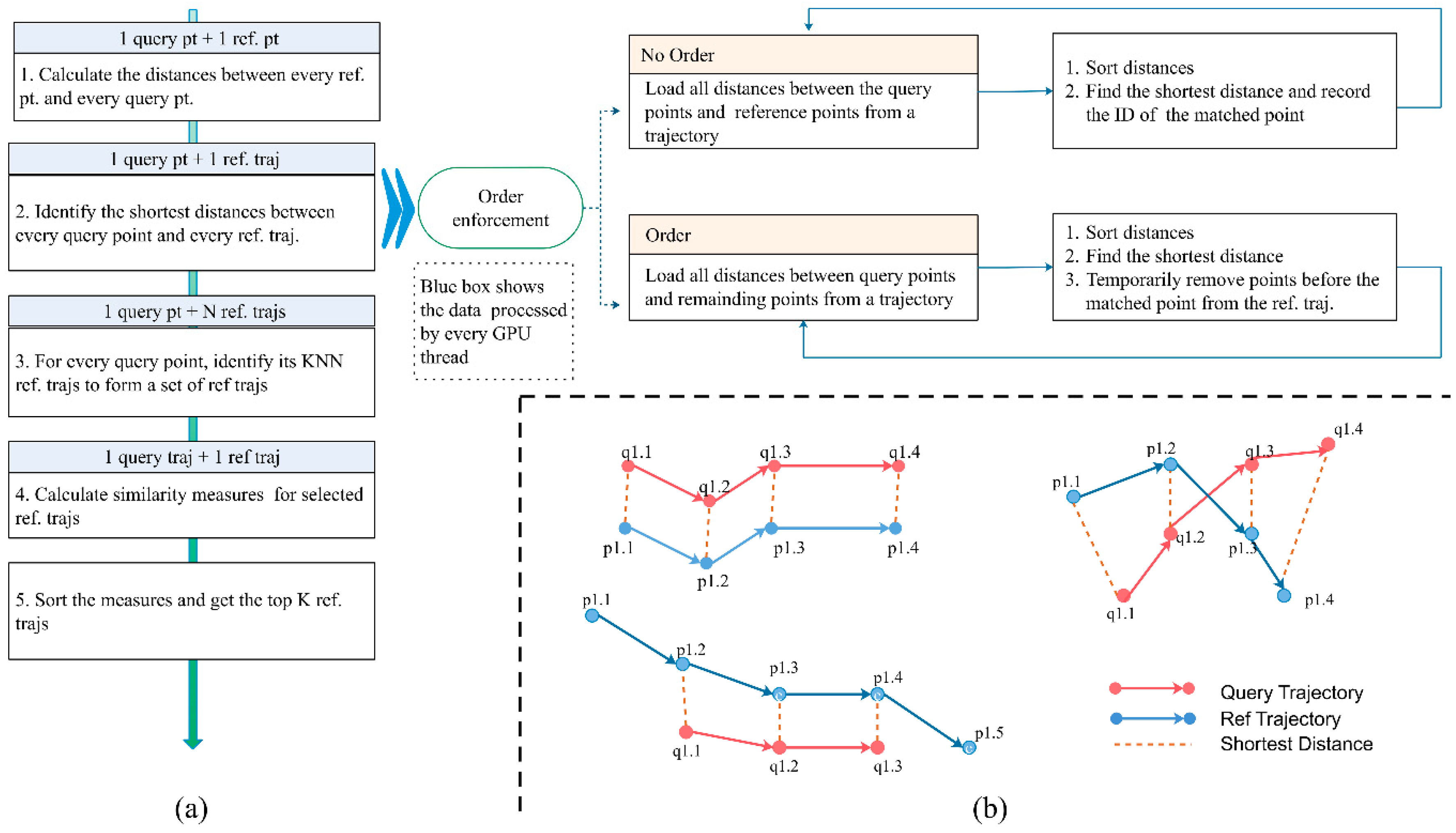
3.1. K-BCT Query: Definition and Basic Implementation Procedure
| Algorithm 1 Parallel k-BCT: identify a top K similar trajectories in parallel |
| Input: |
| //A query trajectory includes an array of query points |
| //A set of reference trajectories. Each trajectory has a list of points |
//A list of reference points |
//Integer, represents the amount of similar trajectories to be identified //Indicates if the order checking is enforced Output: //A list of top K similar trajectories 2DArray: //Compute the Euclidean distances |
| //Identify the top K similar trajectories |
| //from the every query point to every reference trajectory |
// Record the ID of the matched reference point //x is the ID of the reference point // holds the top k trajectory ID else // No need to check ID // holds the top k trajectory ID //Identify the unique trajectories as the candidate trajectories //Calculate similarity Array: |
3.2. Optimizations
3.2.1. Strategy 1: A Progressive MBR and MINDIST Based Filtering Method
- i is the ID of the query point
- m is the total number of query points from the query trajectory
- n1 is the number of checked trajectories
- n2 is the number of total trajectories
- MBR(qi) is the progressive MBR corresponding to the query point i
- MBR(Rj) is the MBR corresponding to the unchecked reference trajectory j
- MD is the MINDIST from the progressive MBR containing a query point to the MBR of an unchecked reference trajectory.
| Algorithm 2 Progressive MBR based MINDIST search |
| Input: |
| //A query trajectory includes an array of query points. |
| //A set of reference trajectories. Each trajectory has a list of points. |
//A list of reference points |
// Minimum distance filter parameter used in Douglas & Peucker algorithm Output: |
| //Sorted IDs of trajectory lists //Sorted MINDST array Array: //Douglas & Peucker algorithm //Identify transitive points //Perform trajectory segmentation to produce a list of sub-trajectories //Calculate the MBRs for every sub trajectory //Calculate the MBRs for every trajectory Array: //Phrase 1 list Array: //Phrase 2 list |
| |
| |
3.2.2. Strategy 2: A Grid-Based MINDIST Shortest Distance Search Method
| Algorithm 3 Grid MINDIST search method for the shortest distance computation |
| Input: |
| //A query trajectory includes an array of query points. //A set of reference trajectories. Each trajectory has a list of points. //A list of reference points |
//Grid configuration data structure, including grid size, grid extent Output: |
| // A list of the shortest distances |
| Initialize G |
Array: //identify the list of grid locations for the trajectory //and the number of points in every grid. |
Array: //Calculate the shortest distance between the grids and query point // is the key //Retrieve all points from the reference trajectory from the grid //Compute the shortest distance between the query points //and the reference points in the grid //Terminate the loop //when the SD is less than the next MD in the array |
3.3. Other Implementation Details
4. Case Study
4.1. Test Datasets and Environments
4.2. Group 1: Serial Processing with CPU and Parallel Processing with GPU
4.3. Group 2: Integrating Progressive MBRs with the Parallel K-BCT Query
4.4. Group 3: Coupling Grid-Based MINDIST Search for SD Computation with the Parallel K-BCT Query
4.5. Summary and Discussion
5. Conclusions and Future Work
Author Contributions
Funding
Acknowledgments
Conflicts of Interest
Abbreviations
| BCT | Best Connected Trajectory |
| CPU | Central Processing Unit |
| GPU | Graphics Processing Unit |
| MBR | Minimum Bounding Rectangle |
| MINDIST | Minimum Distance |
| MSV | Maximum Similarity Value |
| NN | Nearest Neighbor |
| q | Query Trajectory Point |
| Q | Query Trajectory |
| p | Reference Trajectory Point |
| R | Reference Trajectory |
| SD | Shortest Distance |
| SDK | Software Development Kit |
| UTM | Universal Transverse Mercator |
Appendix A

| Query Trajectory | Reference Trajectory | ||||
|---|---|---|---|---|---|
| ID | Number of Query Points | Number of Trajectories | Avg. Number of Points Per Trajectory | Total Points | |
| Group 1 | 1 | 100 | 100 | 90 | 8975 |
| 2 | 100 | 300 | 107 | 32,245 | |
| 3 | 100 | 500 | 132 | 65,992 | |
| 4 | 100 | 700 | 146 | 102,429 | |
| 5 | 200 | 100 | 91 | 9075 | |
| 6 | 200 | 300 | 108 | 32,345 | |
| 7 | 200 | 500 | 132 | 66,092 | |
| 8 | 200 | 700 | 146 | 102,529 | |
| 9 | 300 | 100 | 92 | 9175 | |
| 10 | 300 | 300 | 108 | 32,445 | |
| 11 | 300 | 500 | 132 | 66,192 | |
| 12 | 300 | 700 | 147 | 102,629 | |
| Query Trajectory | Reference Trajectory | |||||||
|---|---|---|---|---|---|---|---|---|
| ID | Number of Query Points | Shape (Straight-Line, Transition) | Location (Near the Center, Cross Multiple Center) | Number of Trajectories | Avg. Number of Points Per Trajectory | Distribution | Total Points | |
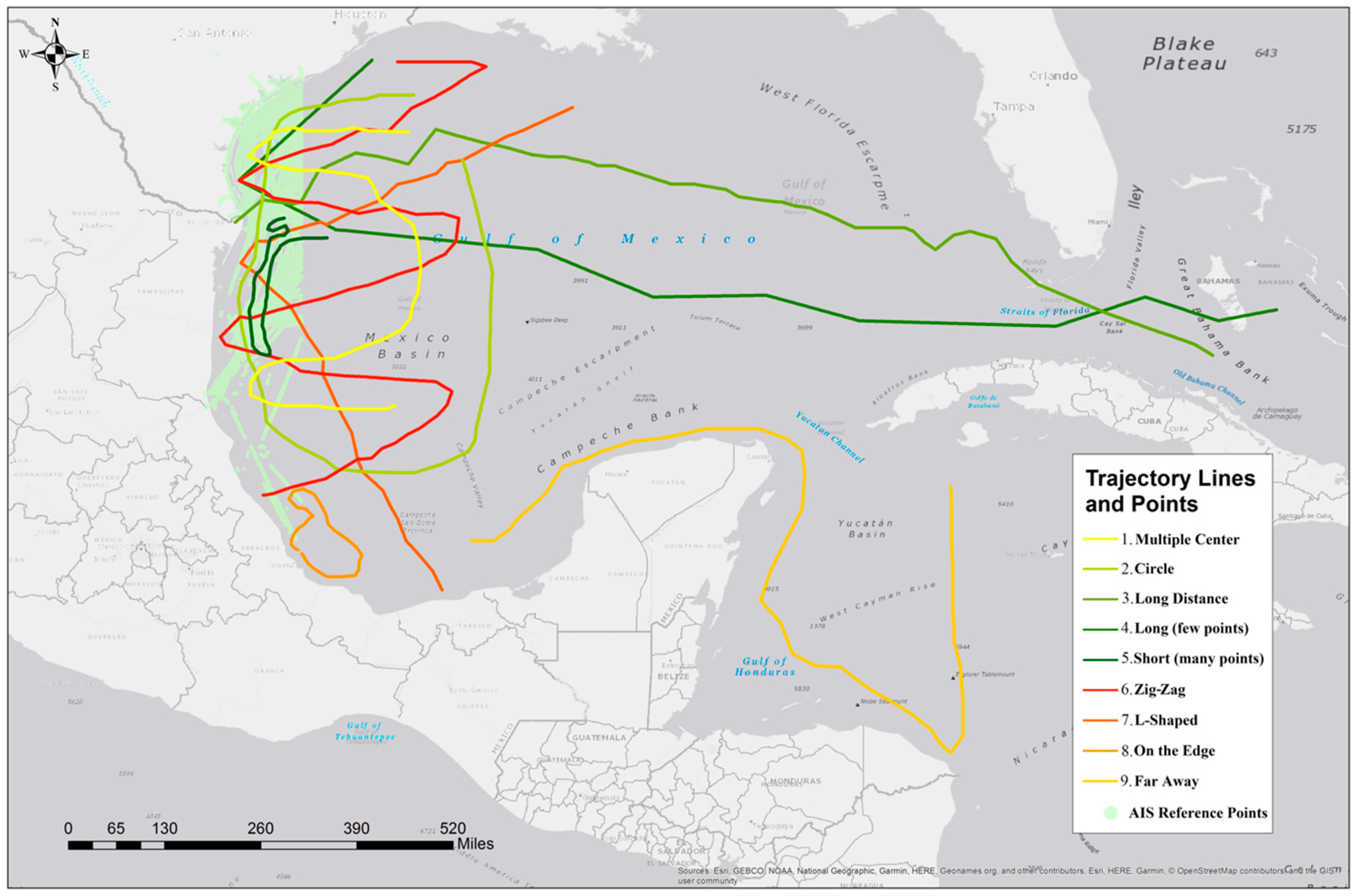
| Group 2 | 1 | 500 | Multiple center | Cross multiple center | 921 | 1305 | Texas | 1,202,073 |
| 2 | 500 | Circle | Cover most points | 921 | 1305 | Texas | 1,202,073 | |
| 3 | 500 | Long distance | Partially connected | 921 | 1305 | Texas | 1,202,073 | |
| 4 | 500 | Short with many points | In the center | 921 | 1305 | Texas | 1,202,073 | |
| 5 | 500 | Zig-zag | Cover most points | 921 | 1305 | Texas | 1,202,073 | |
| 6 | 500 | L-shaped | Cover most points | 921 | 1305 | Texas | 1,202,073 | |
| 7 | 500 | Long with few points | Partially connected | 921 | 1305 | Texas | 1,202,073 | |
| 8 | 500 | Small cluster | Near the edge | 921 | 1305 | Texas | 1,202,073 | |
| 9 | 500 | Far away | Dos not cover any points | 921 | 1305 | Texas | 1,202,073 | |
| Query Trajectory | Reference Trajectory | ||||
|---|---|---|---|---|---|
| ID | Number of Query Points | Number of Trajectories | Avg. Number of Points Per Trajectory | Total Points | |
| Group 3.a | 1 | 735 | 921 | 1305 | 1,202,073 |
| 2 | 507 | 921 | 1305 | 1,202,073 | |
| 3 | 116 | 921 | 1305 | 1,202,073 | |
| 4 | 987 | 921 | 1305 | 1,202,073 | |
| 5 | 6630 | 921 | 1305 | 1,202,073 | |
| Query Trajectory | Reference Trajectory | ||||
|---|---|---|---|---|---|
| ID | Number of Query Points | Number of Trajectories | Avg. Number of Points Per Trajectory | Total Points | |
| Group 3.b | 1 | 292 | 3107 | 430 | 1,336,799 |
| 2 | 933 | 3107 | 430 | 1,336,799 | |
| 3 | 656 | 3107 | 430 | 1,336,799 | |
| 4 | 825 | 3107 | 430 | 1,336,799 | |
| 5 | 924 | 3107 | 430 | 1,336,799 | |
Appendix B
References
- Yuan, J.; Zheng, Y.; Zhang, C.; Xie, W.; Xie, X.; Sun, G.; Huang, Y. T-drive: Driving directions based on taxi trajectories. In Proceedings of the 18th SIGSPATIAL International Conference on Advances in Geographic Information Systems; ACM: New York, NY, USA, 2010; pp. 99–108. [Google Scholar]
- Zheng, Y. Trajectory data mining: An overview. ACM Trans. Intell. Syst. Technol. 2015, 6. [Google Scholar] [CrossRef]
- Tiakas, E.; Papadopoulos, A.N.; Nanopoulos, A.; Manolopoulos, Y.; Stojanovic, D.; Djordjevic-Kajan, S. Searching for similar trajectories in spatial networks. J. Syst. Softw. 2009, 82, 772–788. [Google Scholar] [CrossRef]
- Etienne, L.; Devogele, T.; Buchin, M.; McArdle, G. Trajectory Box Plot: A new pattern to summarize movements. Int. J. Geogr. Inf. Sci. 2016, 30, 835–853. [Google Scholar] [CrossRef]
- Magdy, N.; Sakr, M.A.; Mostafa, T.; El-Bahnasy, K. Review on trajectory similarity measures. In Proceedings of the IEEE 7th International Conference on Intelligent Computing and Information Systems (ICICIS), Cairo, Egypt, 12–14 December 2015. [Google Scholar]
- Deng, K.; Xie, K.; Zheng, K.; Zhou, X. Trajectory indexing and retrieval. In Computing with Spatial Trajectories; Springer: New York, NY, USA, 2011; pp. 35–60. ISBN 978-1-4614-1628-9. [Google Scholar]
- Frentzos, E.; Gratsias, K.; Theodoridis, Y. Index-based most similar trajectory search. In Proceedings of the IEEE 23rd International Conference on Data Engineering, Istanbul, Turkey, 15–20 April 2007. [Google Scholar]
- Gowanlock, M.; Casanova, H. Indexing of spatiotemporal trajectories for efficient distance threshold similarity searches on the GPU. In Proceedings of the IEEE International Parallel and Distributed Processing Symposium, Hyderabad, India, 25–29 May 2015. [Google Scholar]
- Zheng, Y.; Xie, X.; Ma, W.-Y. Geolife: A collaborative social networking service among user, location and trajectory. IEEE Data Eng. Bull. 2010, 33, 32–39. [Google Scholar]
- Lin, B.; Su, J. One way distance: For shape based similarity search of moving object trajectories. GeoInformatica 2008, 12, 117–142. [Google Scholar] [CrossRef]
- Besse, P.; Guillouet, B.; Loubes, J.-M.; François, R. Review and Perspective for Distance Based Trajectory Clustering. arXiv, 2015; arXiv:1508.04904. Available online: http://arxiv.org/abs/1508.04904(accessed on 20 June 2018).
- Arefin, A.S.; Riveros, C.; Berretta, R.; Moscato, P. Gpu-fs-knn: A software tool for fast and scalable knn computation using gpus. PLoS ONE 2012, 7. [Google Scholar] [CrossRef] [PubMed]
- Wang, H.; Su, H.; Zheng, K.; Sadiq, S.; Zhou, X. An effectiveness study on trajectory similarity measures. In Proceedings of the Twenty-Fourth Australasian Database Conference-Volume 137; Australian Computer Society, Inc.: Darlinghurst, Australia, 2013; pp. 13–22. [Google Scholar]
- Mariescu-Istodor, R.; Fränti, P. Grid-based method for GPS route analysis for retrieval. ACM Trans. Spat. Algorithms Syst. 2017, 3. [Google Scholar] [CrossRef]
- Zhang, J.; You, S.; Gruenwald, L. U 2 STRA: High-performance data management of ubiquitous urban sensing trajectories on GPGPUs. In Proceedings of the 2012 ACM Workshop on City data Management Workshop; ACM: New York, NY, USA, 2012; pp. 5–12. [Google Scholar]
- Jacox, E.H.; Samet, H. Spatial join techniques. ACM Trans. Database Syst. 2007, 32. [Google Scholar] [CrossRef]
- Rahat, T.A.; Arman, A.; Ali, M.E. Maximizing reverse k-nearest neighbors for trajectories. In Databases Theory and Applications; Lecture Notes in Computer Science; Springer: Cham, Switzerland, 2018; pp. 262–274. [Google Scholar]
- Lettich, F.; Orlando, S.; Silvestri, C. Processing streams of spatial k-NN queries and position updates on manycore GPUs. In Proceedings of the 23rd SIGSPATIAL International Conference on Advances in Geographic Information Systems; ACM: New York, NY, USA, 2015. [Google Scholar]
- Leal, E.; Gruenwald, L.; Zhang, J.; You, S. Tksimgpu: A parallel top-k trajectory similarity query processing algorithm for gpgpus. In Proceedings of the IEEE International Conference on Big Data (Big Data), Santa Clara, CA, USA, 29 October–1 November 2015. [Google Scholar]
- Papadias, D.; Theodoridis, Y. Spatial relations, minimum bounding rectangles, and spatial data structures. Int. J. Geogr. Inf. Sci. 1997, 11, 111–138. [Google Scholar] [CrossRef]
- Tripathi, P.K.; Debnath, M.; Elmasri, R. A direction based framework for trajectory data analysis. In Proceedings of the 9th ACM International Conference on PErvasive Technologies Related to Assistive Environments; ACM: New York, NY, USA, 2016. [Google Scholar]
- Long, C.; Wong, R.C.-W.; Jagadish, H.V. Direction-preserving trajectory simplification. Proc. VLDB Endow. 2013, 6, 949–960. [Google Scholar] [CrossRef] [Green Version]
- Brox, T.; Malik, J. Object segmentation by long term analysis of point trajectories. In European Conference on Computer Vision; Lecture Notes in Computer Science; Springer: Berlin/Heidelberg, Germany, 2010; pp. 282–295. [Google Scholar]
- Zou, Y.-G.; Fan, Q.-L. OQ-Quad: An efficient query processing for continuous k-nearest neighbor based on quad tree. In Proceedings of the 4th International Conference on Computer Science & Education, Nanning, China, 25–28 July 2009. [Google Scholar]
- Chen, Z.; Shen, H.T.; Zhou, X.; Zheng, Y.; Xie, X. Searching trajectories by locations: an efficiency study. In Proceedings of the 2010 ACM SIGMOD International Conference on Management of Data; ACM: New York, NY, USA, 2010; pp. 255–266. [Google Scholar]
- Waga, K.; Tabarcea, A.; Mariescu-Istodor, R.; Fränti, P. Real time access to multiple GPS tracks. In Proceedings of the 9th International Conference on Web Information Systems and Technologies (WEBIST 2013), Aachen, Germany, 8–10 May 2013; pp. 293–299. [Google Scholar]
- Douglas, D.H.; Peucker, T.K. Algorithms for the reduction of the number of points required to represent a digitized line or its caricature. Cartographica 1973, 10, 112–122. [Google Scholar] [CrossRef]
- Kothuri, R.V.; Ravada, S. Pruning of Spatial Queries Using Index Root MBRS on Partitioned Indexes. U.S. Patent No. 7877405, 25 January 2011. [Google Scholar]
- Wang, H.; Belhassena, A. Parallel trajectory search based on distributed index. Inf. Sci. 2017, 388, 62–83. [Google Scholar] [CrossRef]
- MarineCadastre.gov|Vessel Traffic Data. Available online: https://marinecadastre.gov/ais/ (accessed on 6 June 2018).


| Step | Serial Processing Complexity |
|---|---|
| 1.Distance computation | O(n * m) |
| 2.Shortest distance identification for query points | O(n * (m − M)) |
| 3.Point-based KNN trajectory identification | O(n * K * M’) |
| 4.Similarity calculation using weighted sum of shortest distances | O(m’) + O(M’) |
| 5.Trajectory-based KNN trajectory identification | O(K * M’) |
| Parallelism | Number of Threads | Examples |
|---|---|---|
| Point | number of query points * number of reference points | Brute force distance computation (Step 1); |
| Trajectory | Number of query points * number of reference trajectories Or Number of query points * number of reference trajectories | Shortest distance computation (Step 2); Insert sorting to identify the smallest value in an array of value (Step 5); |
| Dataset | Description | Spatial (Coverage) | Temporal (Frequency, Start and End Time) | Data Pattern |
|---|---|---|---|---|
| AIS: Ship tracks | Data collected from National Automatic Identification System provided by NOAA. | Vessel within U.S. coastal waters. | Data available from 2009 to 2014 at 1 min intervals. | Dataset has high density, trajectory/movements are not restricted in the open ocean. |
| Geolife: GPS tracks of citizens | GPS loggers and GPS-phones to collect trajectories from178 users. | Global | Every 1~5 s (2007–2011) | Dataset has high density, trajectories/movements are restricted by the underlying road network. |
| Mopsi: GPS tracks of citizens | Data collected with GPS-equipped devices from 51 users. | Global | Data collected between 2008 and 2014 | Dataset has lower density and routes record activities such as hiking and biking. |
© 2018 by the authors. Licensee MDPI, Basel, Switzerland. This article is an open access article distributed under the terms and conditions of the Creative Commons Attribution (CC BY) license (http://creativecommons.org/licenses/by/4.0/).
Share and Cite
Li, J.; Wang, X.; Zhang, T.; Xu, Y. Efficient Parallel K Best Connected Trajectory (K-BCT) Query with GPGPU: A Combinatorial Min-Distance and Progressive Bounding Box Approach. ISPRS Int. J. Geo-Inf. 2018, 7, 239. https://doi.org/10.3390/ijgi7070239
Li J, Wang X, Zhang T, Xu Y. Efficient Parallel K Best Connected Trajectory (K-BCT) Query with GPGPU: A Combinatorial Min-Distance and Progressive Bounding Box Approach. ISPRS International Journal of Geo-Information. 2018; 7(7):239. https://doi.org/10.3390/ijgi7070239
Chicago/Turabian StyleLi, Jing, Xuantong Wang, Tong Zhang, and You Xu. 2018. "Efficient Parallel K Best Connected Trajectory (K-BCT) Query with GPGPU: A Combinatorial Min-Distance and Progressive Bounding Box Approach" ISPRS International Journal of Geo-Information 7, no. 7: 239. https://doi.org/10.3390/ijgi7070239