Hexagon-Based Adaptive Crystal Growth Voronoi Diagrams Based on Weighted Planes for Service Area Delimitation


Department of Geography and Geographic Information Science, Natural History Building, 1301 W Green Street, University of Illinois at Urbana-Champaign, Urbana, IL 61801, USA
*
Author to whom correspondence should be addressed.
ISPRS Int. J. Geo-Inf. 2018, 7(7), 257; https://doi.org/10.3390/ijgi7070257
Submission received: 22 May 2018
/
Revised: 7 June 2018
/
Accepted: 26 June 2018
/
Published: 29 June 2018
Abstract
:Delimiting the service area of public facilities is an essential topic in spatial analysis studies. The adaptive crystal growth Voronoi diagrams based on weighted planes are one of the recently proposed methods to address service area delimitation, and consider the geographic distribution of the clients the facilities in question serve and the characteristic of the socioeconomic context, while at the same time mitigate the modifiable areal unit problem when dealing with the socioeconomic context, since the method is based on continuous weighted planes of socioeconomic characteristics rather than arbitrary areal units. However, in the method, the environmental and socioeconomic contexts are rasterized and represented by regular square grids (raster grid). Compared with a raster grid, the hexagon grid tiles the space with regularly sized hexagonal cells, which are closer in shape to circles than to rectangular cells; hexagonal cells also suffer less from orientation bias and sampling bias from edge effects since the distances to the centroids of all six neighbor cells are the same. The purpose of this study is to compare the raster grid and hexagon grid for implementing adaptive crystal growth Voronoi diagrams. With the case study of delimitating middle school service areas, the results are compared based on the raster grid and hexagon grid weighted planes. The findings indicate that the hexagon-based adaptive crystal growth Voronoi diagrams generate better delineation results compared with the raster-based method considering how commensurate the population in each service area is with the enrollment capacity of the middle school in the service area and how accessible the middle schools are within their service areas. The application of hexagon-based adaptive crystal growth Voronoi diagrams may help city managers to serve their citizens better and allocate public service resources more efficiently.
1. Introduction
Delimiting the service areas of public facilities like schools and fire stations is an essential topic in spatial analysis. Geographers and urban planners have considerable theoretical and practical interest in this topic. The methodology of service area delimitation can be applied to address a wide range of issues as evidenced by the literature on the delineation of market areas [1,2,3,4,5,6], school catchment areas [7,8,9,10,11], police districts [12,13,14,15], political districts [16,17,18,19], and service areas of healthcare facilities [12,13,14,15]. There are many existing methods for delimiting service areas, and they can be categorized into mixed-integer programming [6,18,20,21,22,23,24,25] and heuristic approaches (e.g., genetic algorithm [26], simulated annealing, and tabu search [17,27,28,29,30]). Among these methods, Voronoi diagrams, named after Georgy Voronoi, are a popular and promising delimiting method for partitioning space into several subregions based on the distance to a set of seed points specified beforehand [31].
Voronoi diagrams are widely used in the fields of geography and urban planning because of their computational efficiency and effectiveness for delineating the service area of public facilities [32,33,34,35,36]. Based on the ordinary Voronoi diagram, many advanced Voronoi diagrams have been developed to address the complexity of real-world geographic problems, for instance, the weighted Voronoi diagrams that consider the varying service capacities of public facilities [37,38,39], the city Voronoi diagrams that take into account the effect of transport networks and travel time [40], and the adaptive additively weighted Voronoi diagrams that partition a space into subregions with predefined size while considering the position and weight of seed points [38]. More recently, Wang et al. [41] proposed the adaptive crystal growth Voronoi diagrams based on weighted planes, which consider the geographic distribution of the clients the facilities in question serve and the characteristic of the socioeconomic context. The adaptive crystal growth Voronoi diagram approach has several advantages when compared with other heuristic approaches. It distributes demand over continuous space by weighted planes with fine resolution and, thus, more realistically approximates the spatial distribution of demand. It does not rely on population or demand data based on arbitrary administrative units such as census tracts and thus mitigates the modifiable areal unit problem (MAUP) to a certain extent. The approach takes into account not only the transport network but also walkable areas and natural barriers when evaluating accessibility. The method allows for real-time adaptive growth speed of each service area in order to balance the service load according to their capacity for all facilities.
In spatial optimization studies, the representation issues of demand have been extensively discussed [42,43,44,45,46]. There are many ways to spatially represent the demand for service, which include point representation [45], regional representation [47], and area representation [48,49,50]. Murray et al. [46] explored the different configurations of coverage modeling and evaluated the effectiveness of various coverage modeling approaches. The representation of demand for service is one of the critical issues for spatial optimization studies and may influence the quality of the spatial delineation results [42]. For approaches based on an areal representation of demand, there are three kinds of regular polygon grids for covering the land surface without any gap or overlap: equilateral triangles, squares, and hexagons [51]. The equilateral triangular grid is not widely used because the triangles have two different orientations [52] and complex neighbor relationships. For geographic information science (GIS) modeling and spatial analysis, the square grid is widely used due to its symmetric, orthogonal coordinate system which simplifies the calculation and analysis based on the grid as well as its convenience for transformations between different spatial resolutions [52]. Moreover, the pixels of remotely sensed images are based on square grids (or raster grids), so it is more feasible to utilize square grids to integrate other spatial data with remote sensing data.
The hexagon grid data structure is not widely used in GIS and spatial analysis although it has been utilized in different application fields (e.g., the spatial configuration of cell signal coverage) because of its many merits. Different from the equilateral triangle and square grid structure, the hexagon grid is the most complex regular polygon that can fill a land surface without any gap or overlap [52]. Because hexagonal cells are closer to a circle than rectangular cells in terms of their shape [53], they are the most compact regular polygons that tile the land surface, so they “quantize the plane with the smallest average error” and “provide the greatest angular resolution” [54]. Therefore, the hexagon grid can achieve higher accuracy in representing the spatial features of a land surface than can equilateral triangles and square grids from the perspective of spatial analysis [55]. In addition, from the perspective of visualization and cartography, the boundaries of hexagon cells create less distraction when distinguishing spatial patterns because human eyes have a strong response to the horizontal and vertical lines that are naturally generated by equilateral triangles and square grids [51]. Furthermore, the hexagon grid suffers less from orientation bias and sampling bias from edge effects since the distances to the centroids of all six neighboring cells are the same. Tessellated hexagon grids are widely used in ecological research, but less utilized in the spatial optimization problem for several possible reasons: (1) The geometry and spatial configuration of the hexagon gird are more complicated than those of the raster grid and, thus, they increase computational burden. (2) Compared with raster data, there is no mature structure for hexagon grid computation that is ready for use by researchers. (3) Remote sensing data, which is one of the most common data resources, is typically stored as pixels in the regular lattice (raster), so utilizing a hexagon grid to process these data involves the conversion from the raster to the hexagon grid data format, which may introduce errors and render data processing more difficult. (4) Processing spatial data with different resolutions is always needed in spatial analysis. Using different resolutions for a raster grid is relatively straightforward because the composition and decomposition of the raster grid maintain congruency and alignment [52], while it is more complicated for a hexagon grid.
In Wang et al.’s [41] study, the demand for service and the environmental contexts are rasterized and represented by regular square grids (raster grid). Thus, the purpose of this paper is to compare the raster and hexagon grids for implementing adaptive crystal growth Voronoi diagrams. Delimitation results of middle school service areas in the study area based on the raster grid and hexagon grid weighted planes will be compared. The objective of the adaptive crystal growth Voronoi diagrams is to achieve the minimized difference of supply/demand ratio among all the facilities while considering the travel time by actual configuration of accessibility-related context features (e.g., road network, walkable area, and natural barriers). Therefore, whether the population in each service area is commensurate with the enrollment capacity of the corresponding middle school and whether the middle schools are accessible within their service areas are examined. The results indicate that the hexagon-grid-based (hereafter hexagon-based) adaptive crystal growth Voronoi diagrams (HACG) produced superior results to the raster-based one considering how commensurate the population in each service area is with the enrollment capacity of the corresponding middle school (supply/demand ratio) and how accessible each middle school is within its service area (travel time) by addressing both the socioeconomic context and accessibility-related context features when delimiting the service areas of schools.
The remainder of the paper is structured as follows. Section 2 introduces the new hexagon-based adaptive crystal growth Voronoi method for delimiting service area based on socioeconomic factors as well as the conventional raster-based method. Furthermore, a case study is presented in Section 3 to delimit the service area of 34 middle schools in the Haizhu district in Guangzhou, China based on the accessibility-weighted and population-weighted planes. In addition, the delimitation results of the hexagon-based method are compared with those of the raster-based method to show the advantage of the hexagon-based adaptive crystal growth Voronoi diagrams. The paper follows with Section 4, which includes a discussion of the advantages and limitations of the hexagon-based method. Section 5 concludes the paper and also suggests some future research directions.
2. Adaptive Crystal Growth Voronoi Diagrams
This section introduces the conventional adaptive crystal growth Voronoi diagrams based on raster weighted planes as well as the new method based on hexagonal weighted planes. In addition, examples of the raster-based and hexagon-based methods for service area delineation are presented to compare these methods.
2.1. Raster-Based Adaptive Crystal Growth Voronoi Diagrams
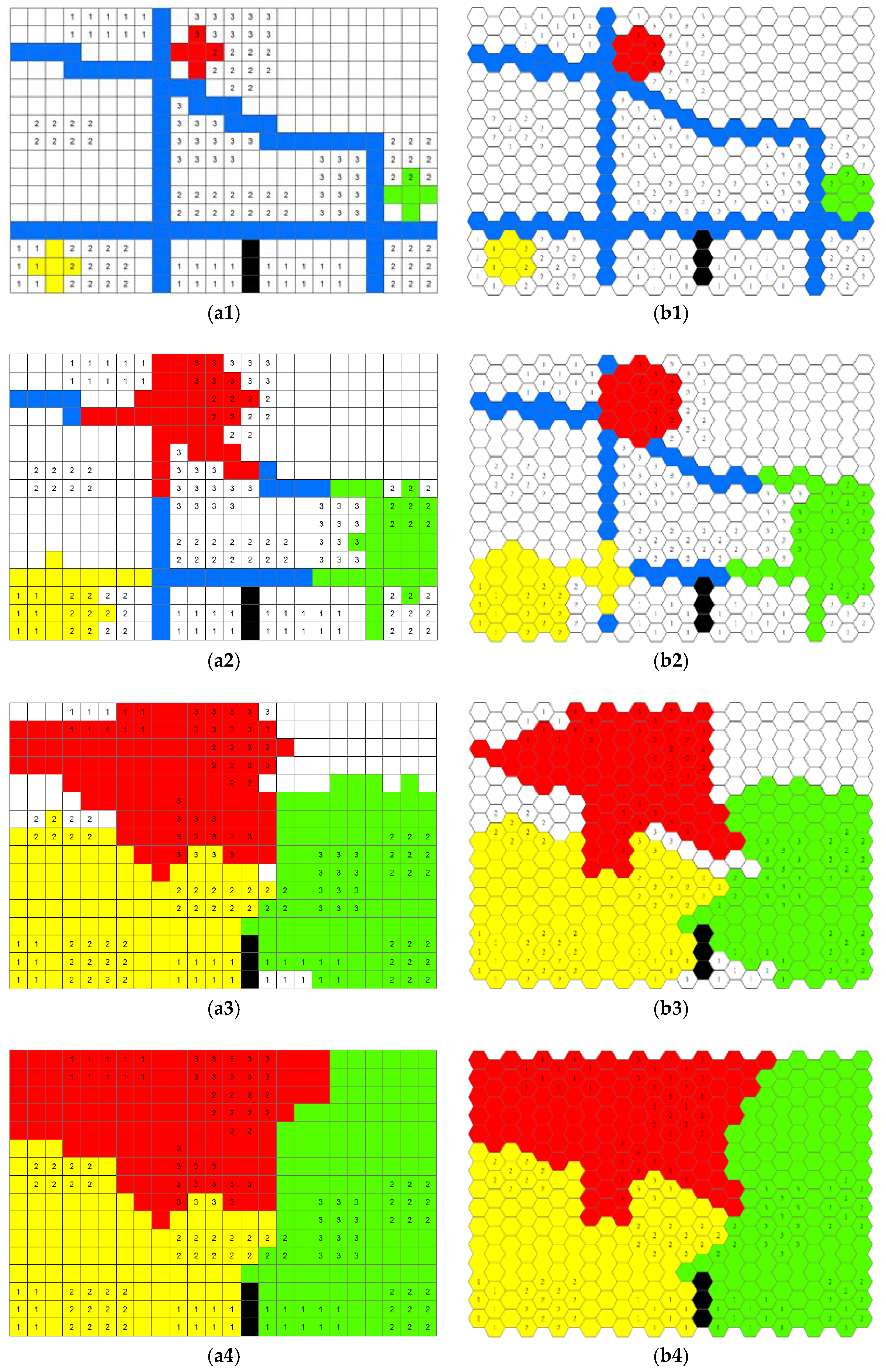
The raster-based adaptive crystal growth Voronoi diagrams (RACG), first proposed by Wang et al. (2014), are an innovative method for delimiting the service areas of public facilities that takes into account the socioeconomic context while mitigating the MAUP. With the middle school service area delineation problem as the case study, the study area was tiled into rectangular cells (raster grid) and two weighted planes (accessibility weighted plane and population distribution weighted plane) were generated based on the raster grid. As illustrated in Figure 1a, on the weighted planes, middle schools were represented as seed points (the cells that intersect with the location of middle schools) with their service capacity as the attribute. The accessibility of the research area (e.g., road network, walkable area, and natural barriers) was simulated as different weight values on the accessibility weighted plane, while the distribution of the population was represented as cells with weights on the population distribution weighted plane. In the method, the Voronoi diagrams are grown simultaneously from all seed point cells (e.g., the location of middle schools), and the service area of each middle school will grow to its neighbor cells cycle by cycle. On the one hand, the growth speed at each location (cell) is adjusted based on the attribute of that cell. For instance, roads speed up the growth while rivers or lakes block the growth. On the other hand, the further growth of any grown area can be either encouraged or constrained in real time according to the service capacity of middle schools and the population coverage of their grown areas (supply/demand ratio). For the purpose of illustration, the distribution of the population is simplified and represented as cell values in Figure 2 with a range of 1 to 3. As shown in the figure, crystal growth starts from the seed point cells to their neighbor cells, and the growth continues cycle by cycle (Figure 2(a1) illustrates one crystal growth cycle). Different from other cells, the growth speed of transport network cells is faster due to the higher accessibility they enable (Figure 2(a1,a2)), while growth is constrained by natural barrier cells because it is normally difficult to pass natural barriers such as rivers and lakes (Figure 2(a2,a3)). As the crystal grows, the population coverage of each grown area is calculated in real time at each crystal growth cycle. According to the population coverage of their grown areas, the growth speed is adaptively adjusted based on specific criteria. For example, if the population size of any grown area is 10% larger than any other grown area, the further growth of this grown area will be temporally stopped until its population size is no more than 10% larger than any other grown area in order to balance the population among all grown areas. The crystal growth concludes when all the cells are grown and assigned to the grown area of one seed point (Figure 2(a4)). The delineation results would be the service area of each seed point (e.g., middle school) considering both the distribution of population and the accessibility of the service region.
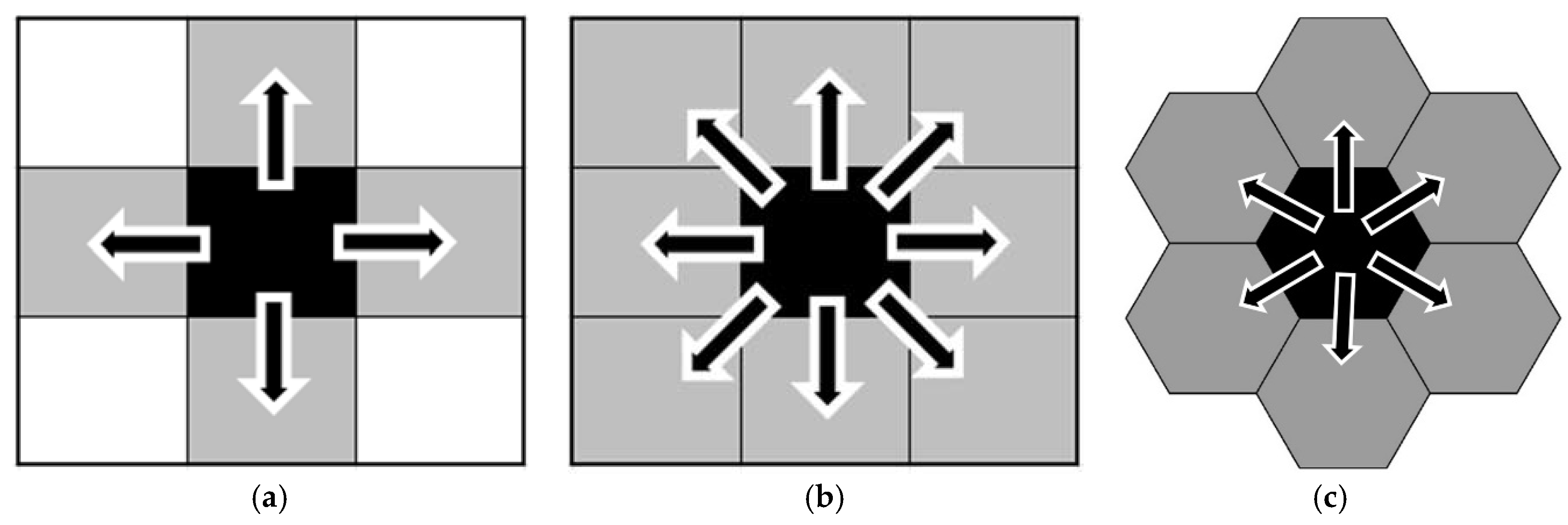
Note that there are two kinds of neighbor cells on the raster-based weighted planes: 4 orthogonal neighbor cells sharing an edge (or “von Neumann neighborhood”) and 4 diagonal neighbor cells sharing a corner (or “Moore neighborhood”). Because the distance to the centroid of diagonal neighbor cells is larger than that to orthogonal neighbor cells, errors will be introduced if the accessibility to these two types of neighbor cells are not treated differently. Therefore, two region-growing algorithms are introduced for the crystal growth Voronoi diagram: a 4-domain region-growing algorithm that only considers the 4 orthogonal neighbor cells and an 8-domain region-growing algorithm that takes into account both kinds of neighbor cells. Figure 3a,b illustrate these two raster-based region-growing algorithms. In Wang et al.’s (2014) method, the 8-domain region-growing algorithm was used for the crystal growth of road network cells due to their high accessibility, while the 4-domain region-growing algorithm was utilized for the crystal growth of other cells.
2.2. Hexagon-Based Adaptive Crystal Growth Voronoi Diagrams
Different from the raster grid, which covers the land surface with continuous rectangular cells arranged in columns and rows, the hexagon grid tiles the space with regularly sized hexagonal cells, which are the most complex regular polygons that can fill the land surface without any gap or overlap [52]. Because hexagonal cells are closer in shape to circles than to rectangular cells, they are more compact in space than rectangular cells [53,55]. Furthermore, the hexagon grid suffers less from orientation bias and sampling bias from edge effects since the distances to the centroids of all six neighbor cells are the same [55]. To the contrary, in a rectangular grid, the distances to the centroids of the 4 neighbor cells that share a corner are longer than the distances to other neighbor cells. Since hexagon cells have only one kind of neighbor cells that share the same edge and have the same distance to their centroids, only one region-growing algorithm is needed for a hexagon grid: a 6-domain region-growing algorithm, which reduces the complication in defining neighbor cells (illustrated in Figure 3c).
Similar to raster-based adaptive crystal growth Voronoi diagrams, the distribution of the socioeconomic variable is represented as cell weights in the hexagon grid. For illustration, the socioeconomic context (e.g., population distribution) is simplified and represented in Figure 1b with a value range of 1 to 3. Figure 2(b1–b4) present an example of the hexagon-based adaptive crystal growth Voronoi diagrams based on weighted planes. As illustrated in Figure 2(b1), the crystal growth starts from the seed point cells based on a 6-domain region-growing algorithm, and the growth continues cycle by cycle. Similar to the raster-based method, the growth speed of transport network cells is faster due to its higher accessibility and growth is constrained by natural barrier cells such as rivers and lakes. The crystal growth speed is adaptively adjusted according to the real-time total weight of each grown area based on the same criteria as for the raster-based adaptive crystal growth Voronoi diagrams illustrated above. As shown in Figure 2, the total weight of the grown area in the final result of the hexagon-based method (Red: 87; Green: 88; Yellow: 88) is more balanced than the total weight of the grown area in the raster-based method (Red: 93; Green: 88; Yellow: 82), which indicates that the hexagon-based adaptive crystal growth Voronoi diagrams may work better in service area delimitation problems.
3. Middle School Service Area Delimitation
In this application, adaptive crystal growth Voronoi diagrams were generated using both raster-based and hexagon-based weighted planes of the same study area with the same socioeconomic context. The results of the HACG will be compared with those of the RACG in delimiting service areas of middle schools using adaptive crystal growth Voronoi diagrams based on accessibility-weighted and population-weighted planes. The delineation results of HACG and RACG are compared in four different spatial resolutions of the weighted plane.
3.1. Study Area
Because of the shortage of educational resources, parents in developing countries face key issues for their children’s education. Under these circumstances, delimitating the service areas of schools is crucial for ensuring an equal and fair distribution of educational resources among the population. In this study, the Haizhu District in Guangzhou, China was selected as the study area because Guangzhou is one of the largest cities in China that faces the problems of both rapid population growth and shortage in educational resources. The Haizhu District in Guangzhou is an island district (Figure 4). It has an area of 90 km2 and a population of about 1.56 million in 2010 based on the sixth nationwide population census of China. There are 34 middle schools and 18 census tracts in the district. As an island, the Haizhu District is relatively independent of other parts of Guangzhou; therefore, choosing it as the study area would help to reduce boundary effects and edge effects in the analysis. Further, its large population and the considerable number of middle schools make it an ideal location for experimenting with middle school service area delineation.
The delineation of the service areas of middle schools is an allocation problem that spatially allocates demand to service facilities. This allocation problem is suitable to be solved by the adaptive crystal growth Voronoi diagram approach because of the following merits of the method: (1) The adaptive crystal growth Voronoi diagrams distribute the population and environmental characteristics over a continuous surface (covered with rectangular or hexagon grids). They thus eliminate the influence of the boundaries of administrative areas (e.g., census tracts) on delineation results and mitigate the MAUP to a certain extent (although the scale of the grid structure (different grid size) may affect the results). (2) The approach takes into account not only the transport network but also walkable areas and natural barriers when evaluating accessibility. (3) The approach allows for real-time adaptive growth speed of each service area in order to balance the service load according to their capacity for all facilities. This is not possible using other methods. (4) Wang et al.’s [41] study has justified that the adaptive crystal growth Voronoi diagram approach performs better when compared with other related methods for school service area delineation. That study uses rectangular grids, and the current study extends the method by using a hexagon-grid-based framework and may obtain further improvement in the results.
3.2. Weighted Planes
Two types of weighted planes, namely an accessibility-based plane and a population-based plane, were generated for each cell structure (raster grid and hexagon grid). In order to explore the scale effects (how the weighted planes in different scales will affect the delineation results), four different spatial resolutions were used for both raster-based and hexagon-based methods; there are thus one accessibility-based plane and one population plane for each cell structure in each spatial resolution. The accessibility-weighted planes take into account the effect of the transport network and water bodies (as natural barriers) on the accessibility of the schools in the study area. The population-weighted planes represent the distribution of population based on distinct types of residential buildings in the study area. The raster and hexagon cells in these weighted planes have the same size in one spatial resolution to ensure consistency and comparability of the results. Four different spatial resolutions of the raster-based and hexagon-based weighted planes are generated to compare the delineating performance. Specifically, these four spatial resolutions include cell sizes of 50, 100, 150, and 200 m2.
For the accessibility-weighted planes, illustrated in Figure 4a, seed point cells are assigned a cell value of 10 with a growth speed of 1 cell/cycle. The natural barrier cells (e.g., rivers and lakes) are assigned a value of 0 with a growth speed of 0 since they are difficult to pass without a road or bridge. The transport cells are assigned a value of 1 to 2, and the growth speed varies with their average travel speed. The growth speed of the primary transport network (e.g., highways, freeways, and primary trunk roads) cells is 6 pixels/cycle for an average driving speed of about 30 km/h, while the growth speed of the secondary transport network (e.g., secondary trunk roads, collector roads, and local roads) cells is 4 pixels/cycle for an average driving speed of about 20 km/h. For all other cells, including walkable area cells, the growth speed is 1 pixel/cycle for an average walking speed of about 5 km/h. The cell attributes of the accessibility-weighted plane are listed in Table 1.
The geographic distribution of the population is one of the major considerations for school service area delimitation in addition to accessibility. Thus, another type of weighted plane for the adaptive crystal growth Voronoi diagrams in this study is based on population distribution. As discussed in Wang et al. (2014), due to the modifiable areal unit problem when using census tracts as the zonal scheme, creating better representations of the continuous distribution of the population is crucial for better results in service area delineations. Therefore, the population-weighted planes in this study were created based on census and land use data, which were used to estimate the population distribution of the research area using the same method in Wang et al. (2014). In the method, the continuous population distribution was simulated by distributing the population from census tracts to each cell in the weighted plane based on the distribution and attributes of residential areas. Residential areas are classified according to an urban land use map and urban planning data into three categories: low-rise residential areas, medium-rise residential areas, and high-rise residential areas. With maximum likelihood estimation, population density is 0.0680 persons/m2 for low-rise residential areas, 0.1135 persons/m2 for medium-rise residential areas, and 0.0937 persons/m2 for high-rise residential areas. Because four different spatial resolutions are used in this study, the cell weights of the population were calculated separately by multiplying the population density with the unit cell size. For instance, with the resolution of 100 m2/cell, the weights of the cells for the three types of residential areas are 6.8 persons/cell (low-rise residential areas), 11.35 persons/cell (medium-rise residential areas), and 9.37 persons/cell (high-rise residential areas) on the weighted plane. Residential cells are assigned a value of 4 (low-rise residence cells), 5 (medium-rise residence cells), or 6 (high-rise residence cells) for the three types of residential areas with a growth speed of 1 cell/cycle. Table 1 lists all the possible cell values and growth speeds on the weighted planes, and Figure 4b illustrates the population-weighted plane.
3.3. Crystal Growth Configuration
In order to make sure that the results of the raster-based and hexagon-based adaptive crystal growth Voronoi diagrams are comparable, the growth rules for both methods are unified as follows:
- (1)
- The seed cells for the raster-based method are the raster cells that intersect with the locations of the 34 middle schools, while the seed point cells for the hexagon-based method are the hexagon cells that intersect with the locations of the 34 middle schools. In the crystal growth process, the service area of each facility grows from the seed point simultaneously.
- (2)
- In each crystal growth cycle of the raster-based method, the 8-domain region-growing algorithm was used for the crystal growth of road network cells due to their high accessibility, while the 4-domain region-growing algorithm was utilized for the crystal growth of other cells. Regarding the hexagon-based method, the 6-domain region-growing algorithm was used.
- (3)
- If a neighbor cell has already been labeled as a grown area or it is a barrier cell, it will be skipped. Otherwise, the neighbor cell will be labeled as a grown area of the specific middle school. Whenever a particular cell is incorporated into the grown service area of a particular seed, it becomes part of that service area. In other words, the calculation is based on the rules of “first come, first served.” If the growth patterns of two service areas come into contact with each other at one place, the growth at that border location will stop for both service areas because the cells beyond that point are already incorporated into either of the service areas. If a cell is claimed by two or more different service areas at the same cycle during the crystal growth process, this cell will be randomly assigned to one of the service areas.
- (4)
- The speed of crystal growth for each cell is determined by the cell value and its growth speed, which was defined on the accessibility-weighted plane. Therefore, the speed is 1 cell per crystal growth cycle for seed point cells, walkable area cells, and residential area cells, while the speed is 4 cells per cycle for secondary transport network cells (the average travel speed on secondary transport network is about 4 times the speed of walking) and 6 cells per cycle for primary transport network cells (the average travel speed on primary transport network is about 6 times the speed of walking).
- (5)
- The growth speed of each grown area is adaptively adjusted in real time to optimize the population in each service area because the population in each service area should be commensurate with the enrollment capacity of each middle school. Therefore, the enrollment capacity of middle schools and the corresponding proportions of enrollment capacity out of the total enrollment capacity in the study area are considered as benchmarks for adjusting the crystal growth speed of each service area. The population of each grown area is calculated based on the population-weighted plane in real time. If the proportion of the population of a grown area () is larger than the proportion of its enrollment capacity () by a defined value (e.g., = 10%), the growth of the corresponding middle school will be restricted:where N is the number of middle schools, is the enrollment capacity of middle schools, is the proportion of enrollment capacity of each middle school out of the total enrollment capacity in the study area, is the population in each grown area, and is the proportion of the population of each grown area out of the total population in all the grown areas.If , then the growth of middle school will be restricted until . is the parameter that defines the strictness of the crystal growth constraint, and it is calibrated to achieve the best result. Generally speaking, the lower the value, the stricter the growth control; the higher the value, the less restrictive the crystal growth. For the specific case study of middle school service areas, the capacity of the service area of each middle school is controlled in the following manner. Equations (1)–(3) are used to calculate the proportion of the population of a grown area () and the proportion of its enrollment capacity () among all middle schools in the study area. Both values are calculated for each grown area after each growth cycle. For any grown service area, if the is larger the by a defined value (e.g., = 10%), the growth of the corresponding middle school will be restricted. In the calculation, the value will iterate from 0.001 to 0.1 in steps of 0.005 to find the best setting for the delineation considering the supply/demand ratio of the results.
- (6)
- The crystal growth will finish if all the accessible cells are grown and assigned to the grown area of one seed point (middle school).
ArcMap was used for the data preprocessing and the hexagon grid generation. The simulation of the service area delineation was implemented with an algorithm we developed based on Python 2.7 and the open source package of Geospatial Data Abstraction Library [56]. The calculation was performed on a Windows 10 desktop computer (CPU: Intel Core i7-6700K 4 GHz; RAM: 16 GB).
3.4. Hexagon Data Structure
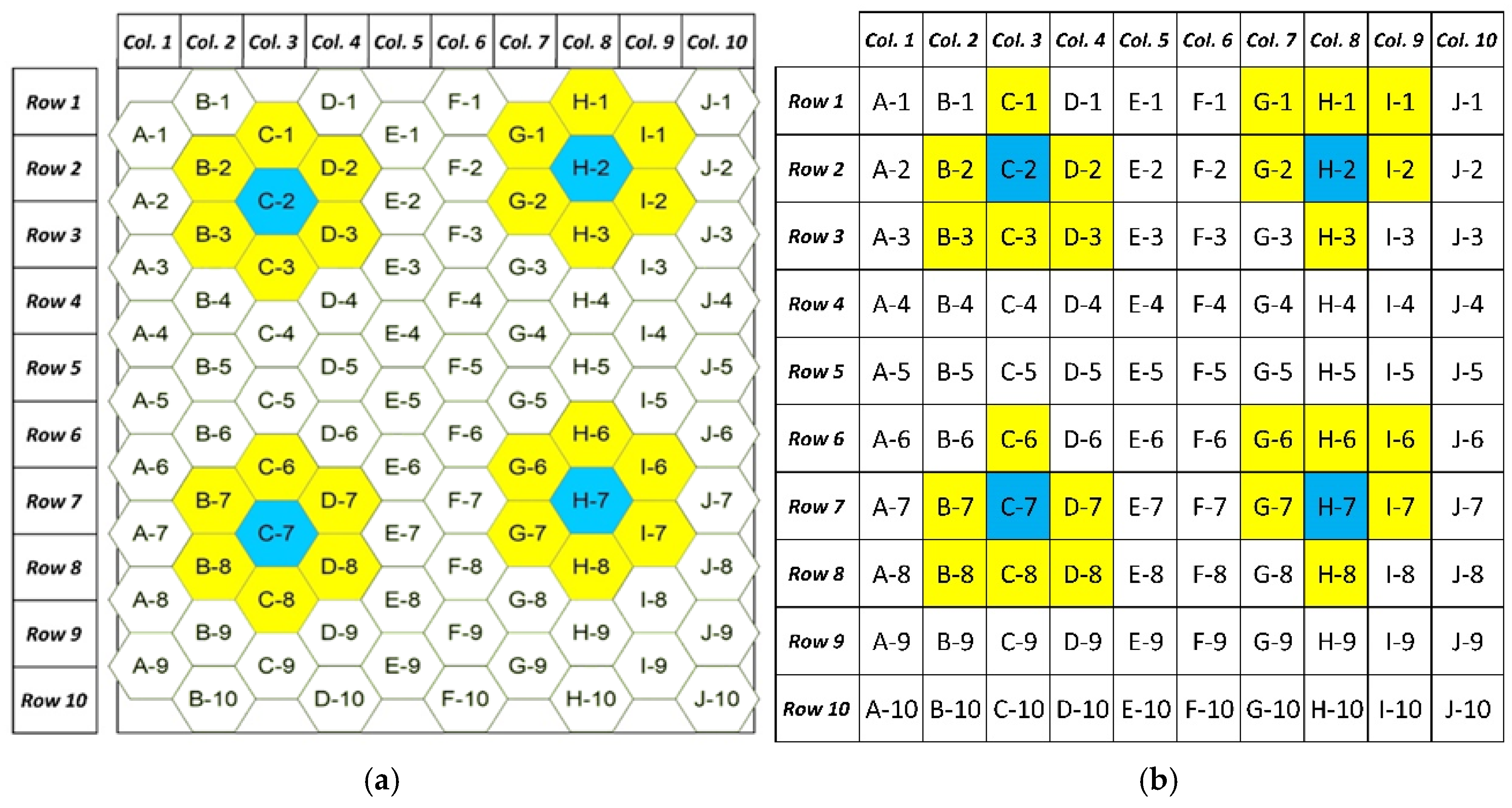
The raster-based weighted planes for RACG are generated based on the widely utilized raster data structure. Nevertheless, there is no mature data structure for hexagon grid computation to the best of our knowledge. The hexagon tessellation implemented by ArcGIS is in the vector format (collection of polygon features), which leads to very low computational efficiency. To address the limitation, we designed a hexagon data structure (we named it “Hexter”) in a similar format to a raster grid but specifically for the crystal growth algorithm to increase the computational efficiency in this study. As illustrated in Figure 5a, the original hexagon grid is indexed as “ColID-RowID”, in which “ColID” represents the index of the column (ranging from “A” to “ZZZ”) in the grid, while “RowID” indicates the index of the row (ranging from “1” to “N”) in the grid. With the indexing, the hexagon grid in the vector format is converted to a raster-like data structure (see the Hexter table in Figure 5b) with their “ColID” as the columns and “RowID” as the rows in the Hexter table. With the change of the data format, the spatial relationship in the table is also changed. Since the only spatial relationship used in the crystal growth algorithm is the neighbor cells, we defined the neighboring relationship of the Hexter based on the original relationship of the hexagon grid. Illustrated in Figure 5b, for the cells in the odd columns (e.g., C, E, and G), the neighbors are the cells in their top, bottom, left, right, bottom-left, and bottom-right (e.g., cells with indices “C-2” and “C-7” in Figure 5), while for the cells in the even columns (e.g., B, D, and F), the neighbors are the cells in their top, bottom, left, right, top-left, and top-right (e.g., cells with indices “H-2” and “H-7” in Figure 5). The rows do not influence the neighboring relationship of cells. Note that the Hexter table does not represent the spatial relationship of hexagon cells. It is only used to read the vector-formatted hexagon grid into the memory in the format of a table for crystal growth computation. After the computation, the crystal growth results (cell values) will be projected to the original hexagon grid by matching the “ColID-RowID”.
3.5. Results
In the study, middle school service areas were delimited by RACG and HACG in four different spatial resolutions (R1: 50 m2; R2: 100 m2; R3: 150 m2; R4: 200 m2) with different settings ranging from 0.001 to 0.1. In order to compare the results, two types of measurements are utilized: (1) how commensurate the population in each service area is with the enrollment capacity of the corresponding middle school; and (2) how accessible each middle school is within its service area.
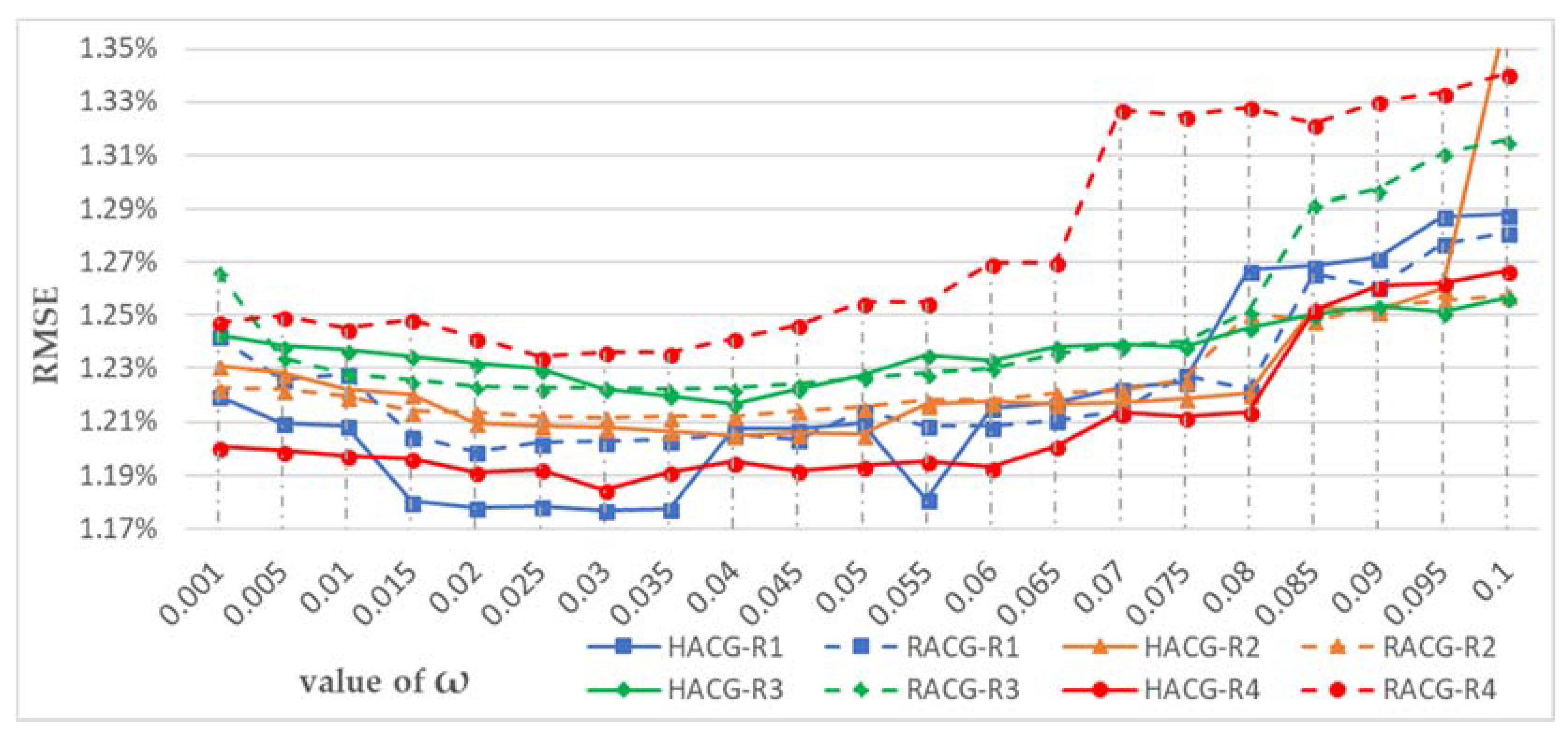
The root-mean-square error (RMSE) and maximum error (Max. Error) are employed to compare the commensurateness between the enrollment capacity of a school and the population of its service area. Figure 6 shows the RMSE of the differences between the proportion of enrollment capacity and the proportion of the population in the service areas delimited by RACG and HACG. It can be seen from the figure that, with different spatial resolutions, the HACG (solid lines in the figure) generally has smaller RMSE compared with the RACG (dashed lines in the figure). In addition, the finer the spatial resolution, the better the results considering the RMSE. In the figure, all lines present a U shape. The best results for different methods and different resolutions are generally achieved when has a value between 0.015 and 0.065. If is larger or smaller than these values, the RMSE increases. For the HACG, the best observed result is achieved when the spatial resolution is 50 m2 and is 0.055 or ranging from 0.015 to 0.035. Similarly, the best observed result is achieved when the spatial resolution is 50 m2 and is between 0.015 and 0.035 for the RACG. However, comparing the two curves of HACG and RACG with the spatial resolution of 50 m2, the delimitation results of the hexagon-based method generally perform better with lower values of RMSE. Figure 7 illustrates the Max. Error of the differences between the proportion of enrollment capacity and the proportion of the population in the service areas delimited by the RACG and HACG with different resolution and settings. Similar with the results of RMSE, the HACG (solid lines in the figure) generally has smaller Max. Error compared with the RACG (dashed lines in the figure) with different spatial resolutions. For both RACG and HACG, the finer the spatial resolution, the smaller the Max. Error. According to the figure, the best observed results for RACG are achieved when is ranging from 0.001 to 0.015, while the best observed results for HACG are achieved when is ranging from 0.02 to 0.08. Considering both the RMSE and Max. Error, the best observed result is obtained when is ranging from 0.02 to 0.035 for HACG, while it is achieved when is 0.015 for RACG. With the best observed values, the HACG has much lower RMSE and Max. Errors compared with the RACG, as shown in the figure. According to the results, both the Max. Errors and RMSE of the differences between the proportion of enrollment capacity and the proportion of population in the service areas are lowest when using the hexagon-based method after calibration of the parameter . Therefore, the results indicate that the hexagon-based method performs better considering the enrollment capacity of middle schools and the population in their service areas.
The longest travel time () to a middle school from any location in its service area is used as a measure of the accessibility to the middle school within its service area in this study. The maximum indicates the lowest accessibility of the middle school in its service area. As discussed above, the best observed results are achieved for both RACG and HACG when the spatial resolution is 50 m2 considering the enrollment capacity of middle schools and the population in their service areas; therefore, the accessibility to the middle school within its service area of the delineation results is only compared using a spatial resolution of 50 m2. Figure 8 shows the maximum of the service areas of all middle schools in the study area based on the delimitation results obtained with different ω settings. For the HACG, the maximum varies with different settings: it stays at high values of around 24 min when , while it is as low as 21 min with other values. Regarding the RACG, the lower values of maximum (around 25 min) are achieved when is smaller than 0.02 and larger than 0.045. Comparing the two curve lines of RACG and HACG, it is clear that HACG always performs better than RACG with smaller maximum .
The mean is the average value of the longest travel time to the middle schools within their service areas, which is used as a general indicator of the accessibility of all middle schools in their service areas based on the delimitation results. Figure 9 illustrates the mean of the service areas of all middle schools based on the delimitation results obtained with different ω settings. The figure shows that the mean for the HACG stays around 8.4 min while it is around 9.4 min for the RACG, but the mean slightly increased with the increase of the value of ω for both methods. Like the maximum , the mean obtained with the RACG is always higher than that obtained with the HACG.
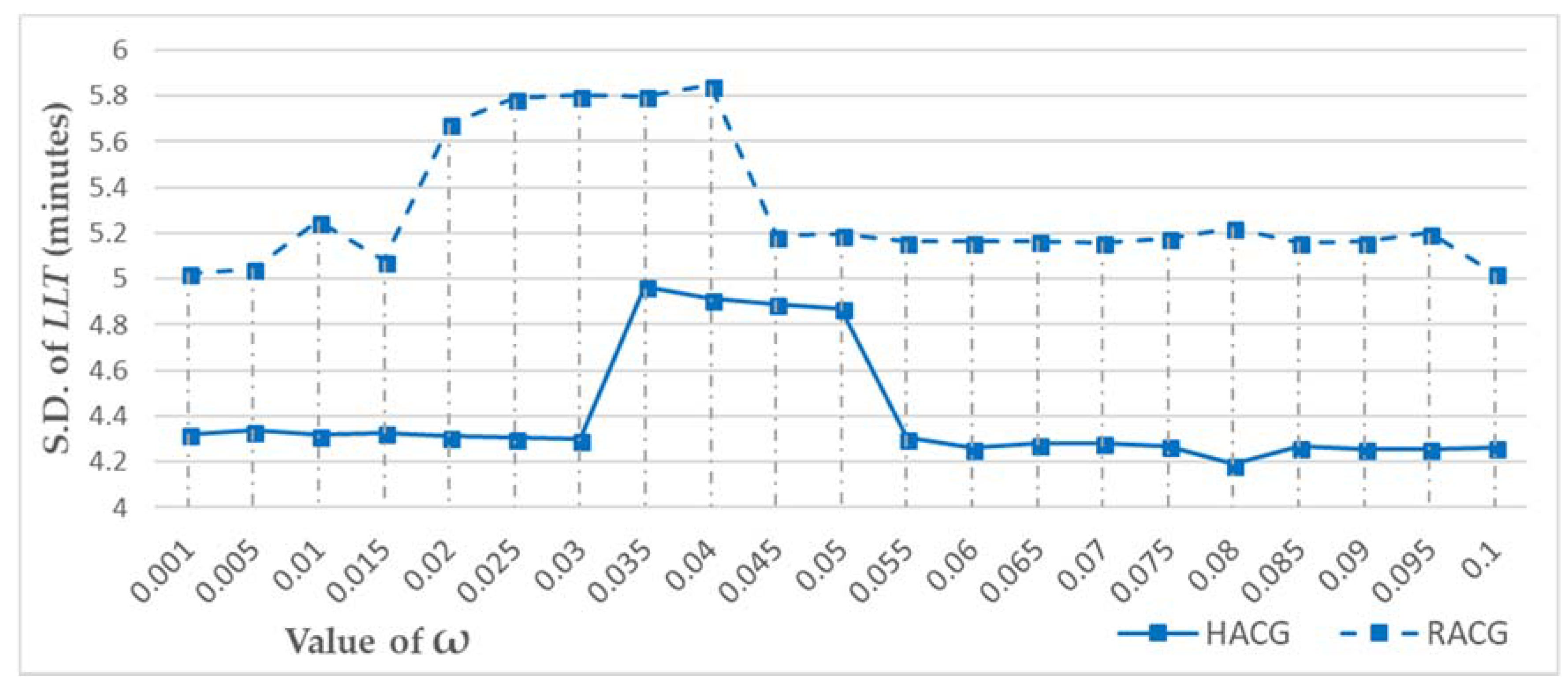
The standard deviation of LTT measures the amount of variation of the longest travel time to the middle schools within their delineated service areas. Figure 10 illustrates the standard deviation of the for all middle schools based on the delineated service areas with different ω settings. Similar to the maximum LTT, for the HACG, the standard deviation of LTT stays at high values of around 4.9 min when . For all the other ω settings, it stays at low values of around 4.2 min. On the contrary, the standard deviation of the LTT obtained with the RACG is always larger than 5 min. Again, the standard deviation of LTT obtained using the RACG is always higher than that obtained with the HACG.
According to the calibration results of the ω settings, the best delimitation results were selected based on how commensurate the population in each service area is with the enrollment capacity of the middle school in the service area and how accessible the middle schools are within their service areas. Thus, the observed best value of ω for the HACG is 0.02, while it is 0.015 for the RACG. Figure 11 illustrates the service area delineation results of the adaptive crystal growth Voronoi diagrams using the raster-based and hexagon-based weighted planes with their respective best observed values. It can be seen from the figure that the results are generally different.
Further, the RMSE and Max. Error of the differences between the proportion of enrollment capacity and the proportion of the population in the service areas, as well as the maximum, mean, and standard deviation of the LTT to a middle school from any location in its service, are compared in Table 2 with the observed best results of both methods. As the table shows, the RMSE, Max. Error, Max. LTT, mean LTT and S.D. LTT are all smaller when using the hexagon-based method compared with their values obtained when using the raster-based method, which also indicates that the HACG performs better than the RACG considering both the commensurate the population in each service area is with the enrollment capacity of the corresponding middle school and the accessibility of each middle school within its service area.
Considering calculation efficiency, Figure 12 illustrates the number of cells for the zoning with different spatial resolutions and their computation time for both raster-based and hexagon-based adaptive crystal growth Voronoi diagrams. It can be seen from the figure that the number of cells increases (from 0.7 to 2.8 million) with finer resolution (from 200 to 50 m2), and the computation time for both methods rises. The computation time for RACG increases from 0.09 to 0.3 min while that for HACG increases from 0.35 to 2.34 min. With the longest computation time of about 2 min with a personal computer, the calculation efficiency for HACG is acceptable and feasible to be utilized in service area delineation problems.
4. Discussion
The best delineation results for HACG and RACG can be obtained by iterating and calibrating the parameter ω. According to the calibration results of the ω settings, the best observed delimitation results were selected based on how commensurate the population in each service area is with the enrollment capacity of the middle school in the service area and how accessible the middle schools are within their service areas. The delimitation results with observed best ω values are illustrated in Figure 11a (RACG) and Figure 11b (HACG). In these figures, the polygons with distinct colors are the service areas of different middle schools. Because the road network, natural barriers, and the population distribution were taken into account through two weighted planes in the adaptive crystal growth Voronoi diagrams, different schools have differently sized service areas; generally speaking, the service area of a middle school is smaller when the road network is sparser, the population density higher, and more natural barriers exist in its surrounding area. Not surprisingly, the shape of some middle schools’ service areas is elongated along the transport network. This is because these middle schools are located in sparsely populated areas where the crystal growth is not constrained and the crystal growth speed along transport network cells is faster than in other cells due to the high accessibility. When comparing the delimitation results of the raster-based and hexagon-based adaptive crystal growth Voronoi diagrams, Figure 11 highlights the fact that these two service area delimitation methods lead to different results with the same crystal growth rules.
Regarding the ω value, which is the only parameter in the method and represents how restrictive the growth constraint rule is, the maximum value of ω for calibration could be defined by the specific question of how great a percentage of service over its capacity for each facility is allowed and tolerable. For instance, considering the middle school service capacity, we require that the service population should not go over its service capacity by 10%. Otherwise, the school would not be able to provide quality education for students. Based on that, the maximum value of ω could be set as 0.1. Therefore, the value can be calibrated in the range from 0 to 0.1. Further, the process to find the optimal ω value is problem-dependent. It depends on the particular service facility in question, and tolerance of errors of the two measurements for the specific questions of (1) how commensurate the population in each service area is with the enrollment capacity of the corresponding middle school (RMSE or Max. Error); and (2) how accessible each middle school is within its service area (Max. or Mean LLT). If the tolerance of errors for how commensurate the population in each service area is with the enrollment capacity of the corresponding middle school is 10%, and the target is to find the optimal results with the least mean LLT, then the calibration procedure is to find the optimal ω value with smallest mean LLT while the Max. Error is no larger than 10%. If the target is to find the best fit of the service population with the enrollment capacity and the tolerance of travel time in each service area is 25 min, then the calibration procedure is to find the optimal ω value with smallest RMSE while the Max. LLT is no larger than 25 min.
The results prove that HACG generates better delineation results than does RACG in many ways. Considering how commensurate the population in each service area is with the enrollment capacity of the corresponding middle school, Figure 6 and Figure 7 show that the proportion of the population in different service areas based on the results of the hexagon-based method is more commensurate with the proportion of middle schools’ enrollment capacity. This may suggest that the hexagon grid may suffer less from orientation bias and sampling bias and thus can generate service areas that better match the service capacities of the middle schools in the study area. Regarding the accessibility of each middle school within its service area, Figure 8, Figure 9 and Figure 10 indicate that the LTT of the service areas delimited by the hexagon-based method is smaller than the LTT of the service areas delimited by the raster-based method. These results indicate that the hexagon-based adaptive crystal growth Voronoi diagrams produced results superior to those obtained with the raster-based diagrams in addressing both the socioeconomic context and accessibility (travel time based on the road network and natural barriers) when delimiting service areas of public schools. Regarding the spatial resolution of the grid cells, the results indicate that the finer the resolution, the better the delineation results for both RACG and HACG. However, with the same resolution, HACG always performs better than RACG.
Although the proposed method extends the adaptive crystal growth Voronoi diagrams and performs better than conventional raster-based methods, there are some limitations which should be addressed in future research. First, a considerable amount of inner-city travel is made by public transit (e.g., bus, subway), which is not considered in this research. It should be integrated into the accessibility-weighted plane to better evaluate the accessibility to public facilities. In addition, all areas are considered as walkable area except buildings, rivers, and lakes, and this is not accurate. Routes that are unsuitable for walking were ignored, and pedestrian sidewalks and pedestrian cut-throughs should be considered in future studies. Further, the socioeconomic weighted plane in this study only considered population distribution; weighted planes of other socioeconomic attributes and new crystal growth rules based on multiple socioeconomic weighted planes are also topics for future research. Lastly, this study is a pilot exploration of the method on school service area delineation to justify the advantages of HACG compared with RACG. However, more studies in different locations with different context settings are needed to investigate the merits and shortcomings of HACG further. Moreover, the method should be further examined in a broader set of test problems in order to be generalizable to the service area delineation of other public facilities.
5. Conclusions
The hexagon-based adaptive crystal growth Voronoi diagram approach for service area delineation presented in this paper represents the most recent and advanced stage in the development of the method by incorporating the newest features, which extends the conventional adaptive crystal growth Voronoi diagrams by utilizing a hexagon-based spatial framework instead of the raster grid structure to represent the demand for service and the environmental contexts. Also, this study found that using a different representation of space (i.e., continuous space covered with hexagonal cells) led to an improvement of the service area delineation results. The results of the middle school service area delineation reveal the advantage of the hexagon-based adaptive crystal growth Voronoi diagrams when compared with the raster-based method, considering both how commensurate the population in each service area is with the enrollment capacity of the corresponding middle school, and how accessible the middle school is within its service area. In the hexagon-based method, the estimated continuous socioeconomic weighted plane mitigates the MAUP, and the hexagon grid accessibility-weighted plane suffers less from orientation bias and sampling bias from edge effects, which may help to delimit service areas that better match the service capacities of public facilities and improve the accessibility of public facilities in their service areas. In the future, other case studies on different kinds of public facilities with varying settings of context will be further explored to see if the conclusion that HACG works better than RACG for service area delineation is generalizable.
The proposed method could provide decision support for policymakers in city management and urban planning (e.g., educational administration) based on robust quantitative analysis results. Although this study implemented hexagon-based adaptive crystal growth Voronoi diagrams for delineating middle school service areas that consider the distribution of population, the method may also be used for delimiting the service area of other public facilities (e.g., fire stations, police stations, and emergency response centers) and may be extended through considering other socioeconomic factors. The hexagon-based adaptive crystal growth Voronoi diagrams and their implementation may help city managers to serve their citizens better and allocate public service resources more efficiently.
Author Contributions
J.W. and M.-P.K. conceived the idea; J.W. designed and performed the experiments and analyzed the data; J.W. wrote the paper; M.-P.K. contributed to refining and revising the paper.
Funding
This research received no external funding.
Acknowledgments
The authors would like to thank the anonymous reviewers for their valuable comments on the manuscript.
Conflicts of Interest
The authors declare no conflict of interest.
References
- Hess, S.W.; Samuels, S.A. Experiences with a Sales Districting Model: Criteria and Implementation. Manag. Sci. 1971, 18, P-41–P-54. [Google Scholar] [CrossRef]
- Shanker, R.J.; Turner, R.E.; Zoltners, A.A. Sales Territory Design: An Integrated Approach. Manag. Sci. 1975, 22, 309–320. [Google Scholar] [CrossRef]
- Marlin, P.G. Application of the transportation model to a large-scale “Districting” problem. Comput. Oper. Res. 1981, 8, 83–96. [Google Scholar] [CrossRef]
- Fleischmann, B.; Paraschis, J.N. Solving a large scale districting problem: A case report. Comput. Oper. Res. 1988, 15, 521–533. [Google Scholar] [CrossRef]
- Sinha, P.; Zoltners, A.A. Sales-Force Decision Models: Insights from 25 Years of Implementation. Interfaces 2001, 31, S8–S44. [Google Scholar] [CrossRef]
- Ríos-Mercado, R.Z.; Fernández, E. A reactive GRASP for a commercial territory design problem with multiple balancing requirements. Comput. Oper. Res. 2009, 36, 755–776. [Google Scholar] [CrossRef]
- Ferland, J.A.; Guénette, G. Decision Support System for the School Districting Problem. Oper. Res. 1990, 38, 15–21. [Google Scholar] [CrossRef] [Green Version]
- Caro, F.; Shirabe, T.; Guignard, M.; Weintraub, A. School Redistricting: Embedding GIS Tools with Integer Programming. J. Oper. Res. Soc. 2004, 55, 836–849. [Google Scholar] [CrossRef]
- Yeates, M. Hinterland delimitation: A distance minimizing approach. Prof. Geogr. 1963, 15, 7–10. [Google Scholar] [CrossRef]
- Franklin, A.D.; Koenigsberg, E. Computed School Assignments in a Large District. Oper. Res. 1973, 21, 413–426. [Google Scholar] [CrossRef]
- Holloway, C.A.; Wehrung, D.A.; Zeitlin, M.P.; Nelson, R.T. An Interactive Procedure for the School Boundary Problem with Declining Enrollment. Oper. Res. 1975, 23, 191–206. [Google Scholar] [CrossRef]
- Steiner, M.T.A.; Datta, D.; Steiner Neto, P.J.; Scarpin, C.T.; Rui Figueira, J. Multi-objective optimization in partitioning the healthcare system of parana state in brazil. Omega 2015, 52, 53–64. [Google Scholar] [CrossRef]
- Benzarti, E.; Sahin, E.; Dallery, Y. Modeling Approaches for the home health care districting problem. In Proceedings of the 8th International Conference of Modeling and Simulation-MOSIM, Hammamet, Tunisia, 10–12 May 2010; pp. 1–10. [Google Scholar]
- Ma, H.; Carlin, B.P.; Banerjee, S. Hierarchical and Joint Site-Edge Methods for Medicare Hospice Service Region Boundary Analysis. Biometrics 2010, 66, 355–364. [Google Scholar] [CrossRef] [PubMed]
- Chen, A.Y.; Yu, T.-Y.; Lu, T.-Y.; Chuang, W.-L.; Lai, J.-S.; Yeh, C.-H.; Oyang, Y.-J.; Heui-Ming Ma, M.; Sun, W.-Z. Ambulance Service Area Considering Disaster-Induced Disturbance on the Transportation Infrastructure. J. Test. Eval. 2015, 43, 20140084. [Google Scholar] [CrossRef]
- Ricca, F.; Scozzari, A.; Simeone, B. Political districting: From classical models to recent approaches. Ann. Oper. Res. 2013, 204, 271–299. [Google Scholar] [CrossRef]
- Bozkaya, B.; Erkut, E.; Laporte, G. A tabu search heuristic and adaptive memory procedure for political districting. Eur. J. Oper. Res. 2003, 144, 12–26. [Google Scholar] [CrossRef]
- Hess, S.W.; Weaver, J.B.; Siegfeldt, H.J.; Whelan, J.N.; Zitlau, P.A. Nonpartisan Political Redistricting by Computer. Oper. Res. 1965, 13, 998–1006. [Google Scholar] [CrossRef]
- George, J.A.; Lamar, B.W.; Wallace, C.A. Political district determination using large-scale network optimization. Socioecon. Plan. Sci. 1997, 31, 11–28. [Google Scholar] [CrossRef]
- Zoltners, A.A.; Sinha, P. Sales Territory Alignment: A Review and Model. Manag. Sci. 1983, 29, 1237–1256. [Google Scholar] [CrossRef]
- Williams, J.C. A Zero-One Programming Model for Contiguous Land Acquisition. Geogr. Anal. 2002, 34, 330–349. [Google Scholar] [CrossRef] [Green Version]
- Shirabe, T. A Model of Contiguity for Spatial Unit Allocation. Geogr. Anal. 2005, 37, 2–16. [Google Scholar] [CrossRef] [Green Version]
- Hakimi, S.L. Optimum Locations of Switching Centers and the Absolute Centers and Medians of a Graph. Oper. Res. 1964, 12, 450–459. [Google Scholar] [CrossRef]
- Hakimi, S.L. Optimum Distribution of Switching Centers in a Communication Network and Some Related Graph Theoretic Problems. Oper. Res. 1965, 13, 462–475. [Google Scholar] [CrossRef]
- Pearce, J. Techniques for defining school catchment areas for comparison with census data. Comput. Environ. Urban Syst. 2000, 24, 283–303. [Google Scholar] [CrossRef]
- Fraley, G.; Jankowska, M.; Jankowski, P. Towards Memetic Algorithms in GIScience: An Adaptive Multi-Objective Algorithm for Optimized Delineation of Neighborhood Boundaries. In Proceedings of the GIScience Conference, Zurich, Switzerland, 9 September 2010; Volume 184. Available online: https://pdfs.semanticscholar.org/21da/8d0d071957c0a4d0fa1a07fa4291f1f2396d.pdf (accessed on 1 May 2018).
- Openshaw, S.; Rao, L. Algorithms for Reengineering 1991 Census Geography. Environ. Plan. A 1995, 27, 425–446. [Google Scholar] [CrossRef] [PubMed]
- Macmillan, W. Redistricting in a GIS environment: An optimisation algorithm using switching-points. J. Geogr. Syst. 2001, 3, 167–180. [Google Scholar] [CrossRef]
- Aerts, J.C.J.H.; Heuvelink, G.B.M. Using simulated annealing for resource allocation. Int. J. Geogr. Inf. Sci. 2002, 16, 571–587. [Google Scholar] [CrossRef] [Green Version]
- D’Amico, S.J.; Wang, S.-J.; Batta, R.; Rump, C.M. A simulated annealing approach to police district design. Comput. Oper. Res. 2002, 29, 667–684. [Google Scholar] [CrossRef]
- Voronoï, G. Nouvelles applications des paramètres continus à la théorie des formes quadratiques. Deuxième mémoire. Recherches sur les parallélloèdres primitifs. J. Reine Angew. Math. 1908, 134, 198–287. [Google Scholar]
- Boyle, P.J.; Dunn, C.E. Redefinition of Enumeration District Centroids: A Test of Their Accuracy by Using Thiessen Polygons. Environ. Plan. A 1991, 23, 1111–1119. [Google Scholar] [CrossRef]
- Boots, B.; South, R. Modeling retail trade areas using higher-order, multiplicatively weighted voronoi diagrams. J. Retail. 1997, 73, 519–536. [Google Scholar] [CrossRef]
- Okabe, A.; Suzuki, A. Locational optimization problems solved through Voronoi diagrams. Eur. J. Oper. Res. 1997, 98, 445–456. [Google Scholar] [CrossRef]
- Zhang, L.; Zhou, H.Y. Research on public establishment location selection based on the voronoi diagram in GIS. Comput. Eng. Appl. 2004, 9, e227. [Google Scholar]
- Zhu, H.; Yan, H.; Li, Y. An optimization method for the layout of public service facilities based on Voronoi diagrams. Sci. Surv. Mapp. 2008, 2, 29. [Google Scholar]
- Schaudt, B.F.; Drysdale, R.L.S. Multiplicatively weighted crystal growth Voronoi diagrams (extended abstract). In Proceedings of the Seventh Annual Symposium on Computational Geometry, North Conway, NH, USA, 10–12 June 1991; ACM Press: New York, NY, USA, 1991; pp. 214–223. [Google Scholar]
- Moreno-Regidor, P.; García López de Lacalle, J.; Manso-Callejo, M.-Á. Zone design of specific sizes using adaptive additively weighted Voronoi diagrams. Int. J. Geogr. Inf. Sci. 2012, 26, 1811–1829. [Google Scholar] [CrossRef] [Green Version]
- Ricca, F.; Scozzari, A.; Simeone, B. Weighted Voronoi region algorithms for political districting. Math. Comput. Model. 2008, 48, 1468–1477. [Google Scholar] [CrossRef]
- Aichholzer, O.; Aurenhammer, F.; Palop, B. Quickest Paths, Straight Skeletons, and the City Voronoi Diagram. Discret. Comput. Geom. 2004, 31, 17–35. [Google Scholar] [CrossRef]
- Wang, J.; Kwan, M.-P.; Ma, L. Delimiting service area using adaptive crystal-growth Voronoi diagrams based on weighted planes: A case study in Haizhu District of Guangzhou in China. Appl. Geogr. 2014, 50, 108–119. [Google Scholar] [CrossRef]
- Murray, A.T. Geography in coverage modelling: Exploiting spatial strucutre to address complementray partial service of areas. Ann. Assoc. Am. Geogr. 2008, 95, 761–772. [Google Scholar] [CrossRef]
- Murray, A.T. Site placement uncertainty in location analysis. Comput. Environ. Urban Syst. 2003, 27, 205–221. [Google Scholar] [CrossRef]
- Church, R.L. Location modelling and GIS. In Geographical Information Systems; Longley, P., Goodchild, M.F., Maguire, D.J., Rhind, D.W., Eds.; John Wiley: Chichester, UK ; Sussex, NJ, USA; New York, NY, USA, 1999; Volume 1, pp. 293–303. [Google Scholar]
- Miller, H.J. GIS and geometric representation in facility location problems. Int. J. Geogr. Inf. Syst. 1996, 10, 791–816. [Google Scholar] [CrossRef]
- Murray, A.T.; O’Kelly, M.E.; Church, R.L. Regional service coverage modeling. Comput. Oper. Res. 2008, 35, 339–355. [Google Scholar] [CrossRef]
- Suzuki, A.; Drezner, Z. The p-center location problem in an area. Locat. Sci. 1996, 4, 69–82. [Google Scholar] [CrossRef]
- Bennett, C.D.; Mirakhor, A. Optimal facility location with respect to several regions. J. Reg. Sci. 1974, 14, 131–136. [Google Scholar] [CrossRef]
- Aly, A.A.; Marucheck, A.S. Generalized Weber problem with rectangular regions. J. Oper. Res. Soc. 1982, 33, 983–989. [Google Scholar] [CrossRef]
- Love, R.F. A computational procedure for optimally locating a facility with respect to several rectangular regions. J. Reg. Sci. 1972, 12, 233–242. [Google Scholar] [CrossRef]
- Carr, D.B.; Olsen, A.R.; White, D. Hexagon Mosaic Maps for Display of Univariate and Bivariate Geographical Data. Cartogr. Geogr. Inf. Sci. 1992, 19, 228–236. [Google Scholar] [CrossRef]
- Birch, C.P.D.; Oom, S.P.; Beecham, J.A. Rectangular and hexagonal grids used for observation, experiment and simulation in ecology. Ecol. Modell. 2007, 206, 347–359. [Google Scholar] [CrossRef]
- Feick, R.; Robertson, C. A multi-scale approach to exploring urban places in geotagged photographs. Comput. Environ. Urban Syst. 2015, 53, 96–109. [Google Scholar] [CrossRef]
- Sahr, K.; White, D.; Kimerling, A.J. Geodesic Discrete Global Grid Systems. Cartogr. Geogr. Inf. Sci. 2003, 30, 121–134. [Google Scholar] [CrossRef]
- Zook, M. Small Stories in Big Data: Gaining Insights from Large Spatial Point Pattern Datasets. Cityscape J. Policy Dev. Res. 2015, 17, 151–160. [Google Scholar]
- GDAL—Geospatial Data Abstraction Library. Available online: http://gdal.org (accessed on 1 May 2018).
Figure 1.
Illustration of raster-based (a) and hexagon-based (b) weighted planes. The numbers in the grid cells are the weights representing the spatial distribution of a socioeconomic factor (e.g., population). The blue cells represent elements of the road network; the black cells represent natural barriers; the red, green, and yellow cells are three seed cells representing public service facilities (e.g., middle schools).

Figure 2.
Illustration of the adaptive crystal growth Voronoi diagrams with raster-based (a1–a4) and hexagon-based (b1–b4) weighted planes. The weights for all grown areas (served population) of the final delineation results are concluded as follows: Red: 93, Green: 88, and Yellow: 82 for the raster-based method; Red: 87, Green: 88, and Yellow: 88 for the hexagon-based method.

Figure 3.
The 4-domain (a) and 8-domain (b) region-growing algorithms for the raster grid; and the 6-domain (c) region-growing algorithm for the hexagon grid.
Figure 3.
The 4-domain (a) and 8-domain (b) region-growing algorithms for the raster grid; and the 6-domain (c) region-growing algorithm for the hexagon grid.

Figure 4.
The location of the study area—Haizhu, Guangzhou (the background map was abstracted from Google Maps)—and the illustration of the population-weighted plane (a) and accessibility-weighted plane (b).
Figure 4.
The location of the study area—Haizhu, Guangzhou (the background map was abstracted from Google Maps)—and the illustration of the population-weighted plane (a) and accessibility-weighted plane (b).


Figure 5.
The original hexagon grid in the vector format (a) and transformed hexagon grid in the “Hexter” data structure (b) with an illustration of the neighbor cells definition. The illustrated center cells are colored in blue while their immediate neighbor cells are colored in yellow.
Figure 5.
The original hexagon grid in the vector format (a) and transformed hexagon grid in the “Hexter” data structure (b) with an illustration of the neighbor cells definition. The illustrated center cells are colored in blue while their immediate neighbor cells are colored in yellow.

Figure 6.
The root-mean-square error (RMSE) of the differences between the proportion of enrollment capacity and the population proportion of service areas with different ω settings. RACG: raster-based adaptive crystal growth method. HACG: hexagon-based adaptive crystal growth method.
Figure 6.
The root-mean-square error (RMSE) of the differences between the proportion of enrollment capacity and the population proportion of service areas with different ω settings. RACG: raster-based adaptive crystal growth method. HACG: hexagon-based adaptive crystal growth method.

Figure 7.
The maximum error of the differences between the proportion of enrollment capacity and the population proportion of service areas with different ω settings.
Figure 7.
The maximum error of the differences between the proportion of enrollment capacity and the population proportion of service areas with different ω settings.

Figure 8.
Maximum longest travel time ( of service areas based on the delimiting results with different ω settings.
Figure 8.
Maximum longest travel time ( of service areas based on the delimiting results with different ω settings.

Figure 9.
Mean of service areas based on the delimiting results with different ω settings.

Figure 10.
The standard deviation of of service areas for all middle schools based on the delimiting results with different ω settings.
Figure 10.
The standard deviation of of service areas for all middle schools based on the delimiting results with different ω settings.

Figure 11.
The delineation result of middle school service areas by using raster-based (a) and hexagon-based (b) adaptive crystal growth Voronoi diagrams.
Figure 11.
The delineation result of middle school service areas by using raster-based (a) and hexagon-based (b) adaptive crystal growth Voronoi diagrams.

Figure 12.
The computation efficiency of the raster-based (blue) and hexagon-based (orange) adaptive crystal growth Voronoi diagrams for different spatial resolutions. (The left vertical axis is the computation time in minutes, while the right vertical axis is the number of cells for the weighted planes with different resolution.)


Table 1.
Cell values and weights of the accessibility-weighted and population-weighted planes.
| Cell Type | Cell Value | Growth Speed | |
|---|---|---|---|
| Accessibility-weighted plane | Natural Barrier Cells | 0 | 0 |
| Primary Transport Network Cells | 1 | 6 pixels/cycle | |
| Secondary Transport Network Cells | 2 | 4 pixels/cycle | |
| Walkable Area Cells | 3 | 1 pixel/cycle | |
| Population-weighted plane | Low-Rise Residential Cells | 4 | 1 pixel/cycle |
| Medium-Rise Residential Cells | 5 | 1 pixel/cycle | |
| High-Rise Residential Cells | 6 | 1 pixel/cycle | |
| Seed Point Cells (Middle Schools) | 10 | 1 pixel/cycle |
Table 2.
Comparison of the differences between the proportion of enrollment capacity of each middle school and the proportion of the population in each service area of the 34 middle schools in the observed best delimitation results (ω = 0.015 for RACG; ω = 0.02 for HACG).
Table 2.
Comparison of the differences between the proportion of enrollment capacity of each middle school and the proportion of the population in each service area of the 34 middle schools in the observed best delimitation results (ω = 0.015 for RACG; ω = 0.02 for HACG).
| RMSE | Max. Error | Max. LTT | Mean LTT | S.D. LTT | |
|---|---|---|---|---|---|
| RACG | 1.2048% | 3.0379% | 25.6759 | 9.2379 | 5.0803 |
| HACG | 1.1779% | 2.9833% | 21.7985 | 8.2283 | 4.3100 |
Note: RACG represents the raster-based adaptive crystal growth Voronoi diagram; HACG represents the hexagon-based adaptive crystal growth Voronoi diagram.
© 2018 by the authors. Licensee MDPI, Basel, Switzerland. This article is an open access article distributed under the terms and conditions of the Creative Commons Attribution (CC BY) license (http://creativecommons.org/licenses/by/4.0/).
Share and Cite
MDPI and ACS Style
Wang, J.; Kwan, M.-P. Hexagon-Based Adaptive Crystal Growth Voronoi Diagrams Based on Weighted Planes for Service Area Delimitation. ISPRS Int. J. Geo-Inf. 2018, 7, 257. https://doi.org/10.3390/ijgi7070257
AMA Style
Wang J, Kwan M-P. Hexagon-Based Adaptive Crystal Growth Voronoi Diagrams Based on Weighted Planes for Service Area Delimitation. ISPRS International Journal of Geo-Information. 2018; 7(7):257. https://doi.org/10.3390/ijgi7070257
Chicago/Turabian StyleWang, Jue, and Mei-Po Kwan. 2018. "Hexagon-Based Adaptive Crystal Growth Voronoi Diagrams Based on Weighted Planes for Service Area Delimitation" ISPRS International Journal of Geo-Information 7, no. 7: 257. https://doi.org/10.3390/ijgi7070257
Note that from the first issue of 2016, this journal uses article numbers instead of page numbers. See further details here.