Shared Execution Approach to ε-Distance Join Queries in Dynamic Road Networks

Abstract

Given a threshold distance ε and two object sets R and S in a road network, an ε-distance join query finds object pairs from R × S that are within the threshold distance ε (e.g., find passenger and taxicab pairs within a five-minute driving distance). Although this is a well-studied problem in the Euclidean space, little attention has been paid to dynamic road networks where the weights of road segments (e.g., travel times) are frequently updated and the distance between two objects is the length of the shortest path connecting them. In this work, we address the problem of ε-distance join queries in dynamic road networks by proposing an optimized ε-distance join algorithm called EDISON, the key concept of which is to cluster adjacent objects of the same type into a group, and then to optimize shared execution for the group to avoid redundant network traversal. The proposed method is intuitive and easy to implement, thereby allowing its simple integration with existing range query algorithms in road networks. We conduct an extensive experimental study using real-world roadmaps to show the efficiency and scalability of our shared execution approach.

1. Introduction

Recent advances in mobile technologies and map-based applications enable users to access a wide range of location-based services such as shortest path queries [1,2,3,4,5,6,7], distance queries [2,3,5,8,9], range queries [3,10], and k-nearest neighbor (kNN) queries [3,7,10,11,12]. Owing to the popularity of map-based applications among users, processing spatial queries in road networks efficiently has become an important research area in recent years. In this work, we address $\epsilon$-distance join queries in road networks. Given a threshold distance $\epsilon$ and two object sets $R$ and $S$, an $\epsilon$-distance join query explores all object pairs $\left(r,s\right)\in R\times S$ and returns a set of object pairs $\left(r,s\right)$ that are within the threshold distance $\epsilon$. The $\epsilon$-distance join queries are useful in real-life applications such as data mining and similarity joins [13,14,15,16,17,18]. Therefore, many studies have evaluated the efficiency of $\epsilon$-distance join queries in the Euclidean space [19,20] and in the metric space [13,14,15,16,17,18]. These studies focus primarily on designing elegant indexing techniques to avoid scanning the entire dataset repeatedly, and on pruning as many distance computations as possible.

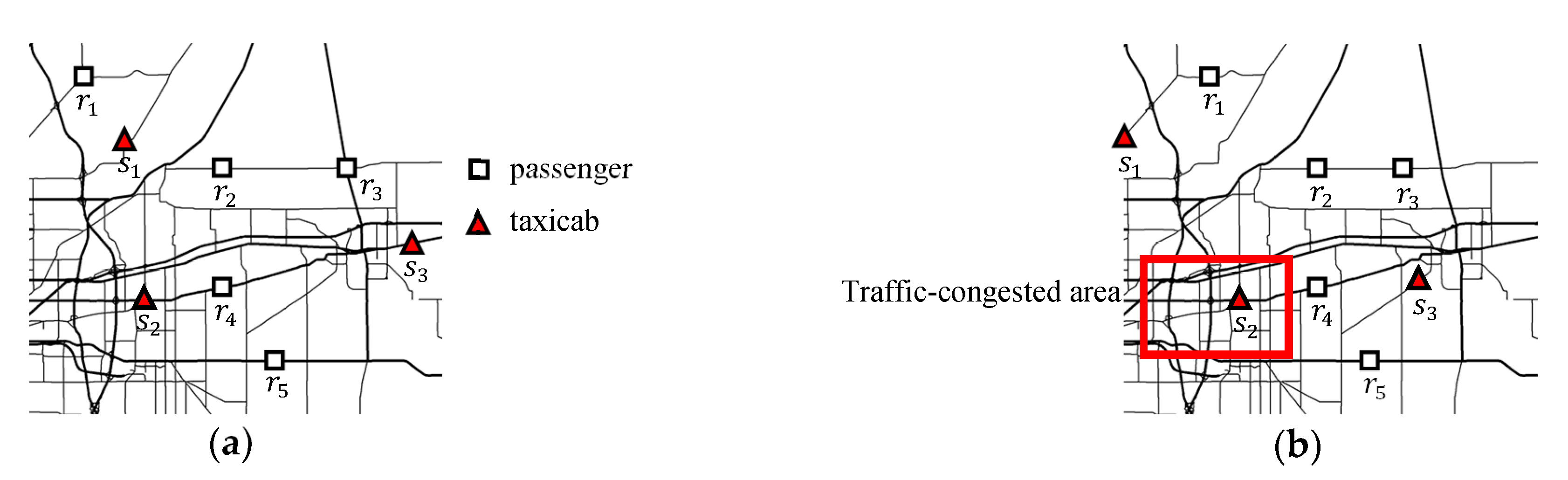
Figure 1 presents an example of dynamic road networks where objects $r_1$ through $r_5$ denote passengers (represented by rectangles), and objects $s_1$ through $s_3$ denote taxicabs (represented by triangles). In this example, an $\epsilon$-distance join query for a taxicab company involves sending an available taxicab to each passenger who is located within a five-minute driving distance from the taxicab. The travel time should be frequently updated depending on traffic conditions. For example, at time $t_1$, taxicab $s_2$ is closer to passenger $r_4$ than taxicab $s_3$, as shown in Figure 1a. However, as shown in Figure 1b, because the taxicab $s_2$ is in a traffic-congested area, it cannot reach the passenger $r_4$ faster than the taxicab $s_3$ at time $t_2$.

Owing to the dynamic nature of road networks, many studies have recently addressed a variety of spatial queries in dynamic road networks such as shortest path queries [1,6,21], distance queries [8], and kNN queries [22]. Although there have been a few studies [10,23] on $\epsilon$-distance join queries in road networks, they proposed sophisticated index structures and algorithms to boost $\epsilon$-distance join queries in static road networks, where the weights of road segments are rarely updated. Specifically, the state-of-the-art solution to $\epsilon$-distance join queries in road networks is the distance join algorithm proposed in Reference [23], based on the spatially induced linkage cognizance (SILC) framework introduced in Reference [3]. The algorithm pre-computes the shortest path between each pair of vertices in a road network and stores all paths. This approach is not suitable for dynamic road networks because in these road networks, the weights of road segments are frequently updated, and the pre-computed distances between vertices often become obsolete. Various techniques [24,25,26,27,28,29,30,31,32,33,34] for preserving location privacy in road networks have recently been developed, which focus on moving objects such as vehicles and users, and therefore cannot be applied to the problem studied here.

Therefore, in this study, we propose an optimized $\epsilon$-distance join algorithm called EDISON to efficiently support $\epsilon$-distance join queries in dynamic road networks, where materialized structures such as the SILC framework cannot be used to dynamically compute the shortest path and distances from a source point to one or more destination points. Intuitively, a simple solution involves computing the distance between every object pair from two datasets. This simple solution is very inefficient, because for each element in an object set $R$, the algorithm must traverse another object set $S$, which can lead to redundant network traversal. The proposed solution is to cluster adjacent objects of the same type into a group and then optimize shared execution for the group to avoid redundant network traversal. Although the shared execution of queries has received much attention [21,35,36,37,38], no shared execution strategy has been applied to evaluate $\epsilon$-distance join queries in dynamic road networks to date. The contributions of this study are as follows.

• We propose an efficient $\epsilon$-distance join algorithm called EDISON for dynamic road networks that optimizes the shared execution paradigm to accelerate query response times. To the best of our knowledge, this is the first attempt to evaluate $\epsilon$-distance join queries effectively in dynamic road networks.
• We design algorithms that reduce the number of range queries required to evaluate $\epsilon$-distance join queries in dynamic road networks. The proposed method is intuitive and easy to implement, thereby allowing its simple integration with existing range query algorithms (e.g., [10]) in road networks.
• We conduct extensive experiments under different setups to demonstrate the efficiency and scalability of our approach over conventional solutions.

The remainder of this paper is organized as follows. In Section 2, we review related studies. In Section 3, we provide some background information. We present a simple solution called the naive EDISON method based on shared execution in Section 4. In Section 5, we present an optimized solution that avoids redundant network traversal called the EDISON method. In Section 6, we evaluate our proposed solutions experimentally under different setups by comparing them to a conventional solution. We conclude the paper in Section 7.

2. Related Work

2.1. Dynamic Road Networks

The geographic information system (GIS) community has shown interest in processing spatial queries in road networks, which form an integral aspect of geospatial applications, such as location-based services and locational analysis [1,2,3,5,6,7,10,11,22,23,39,40]. Previous works have studied a variety of spatial queries in road networks, which include shortest path queries [1,2,3,4,5,6,7], distance queries [2,3,5,8,9], range queries [3,10], and kNN queries [3,7,10,11]. The previous studies focused primarily on adopting sophisticated index structures to achieve good performance under the assumption that road networks are stable. For example, Sankaranarayanan et al. [3,4] proposed the SILC and path-coherent pairs decomposition frameworks based on spatial path coherence to determine the shortest path and the shortest distance between every pair of vertices. In particular, the SILC framework can support various queries in road networks including path queries, distance queries, range queries, and kNN queries. Because these frameworks have high pre-computational overhead and space complexity even in static road networks, they are not suitable for processing spatial queries in dynamic road networks where the weights of road segments are often updated. Recently, distance queries [8] and shortest path queries [1,6,21] have been actively studied in dynamic road networks. Techniques for distance queries and shortest path queries cannot be applied directly to processing $\epsilon$-distance join queries in dynamic road networks owing to the inconsistent problem requirements. Recently, Arain et al. [24,25,26], Domenic et al. [27], Gustav et al. [28], Kamenyi et al. [29], and Memon et al. [30,31,32,33,34] developed novel techniques for location privacy preservation over road networks. These techniques focus on protecting the location privacy of moving objects in road networks. However, it is inappropriate to extend these location privacy techniques to solve the $\epsilon$-distance join problem in dynamic road networks owing to differences in the problem definition.

2.2. $\epsilon$-Distance Join Queries

Given a query point $q$, a threshold distance $\epsilon$, and a set of objects $S$, a range query retrieves objects that are within the threshold distance $\epsilon$ from the query point $q$. Several algorithms have been proposed to support range queries in road networks. Papadias et al. [10] proposed the range Euclidean restriction (RER) and range network expansion (RNE) algorithms for processing range queries in road networks. The $\epsilon$-distance join query is another important query in road networks. Papadias et al. [10] proposed join Euclidean restriction (JER) and join network expansion (JNE) algorithms to support $\epsilon$-distance join queries in road networks. The JER algorithm uses the Euclidean distance as a heuristic to search for object pairs within the threshold distance $\epsilon$ based on their network distance. Therefore, it performs poorly when the Euclidean distance and the network distance are very different, which is a common scenario in practice. If the edge weight is defined as the travel time in road networks, the Euclidean distance cannot confine the search space unless additional assumptions are made, such as assuming maximum speed. Therefore, JER is not appropriate for processing $\epsilon$-distance join queries in dynamic road networks. Sankaranarayanan et al. [23] proposed a distance join algorithm that can support $\epsilon$-distance join queries in road networks. The distance join algorithm, based on the SILC framework introduced in [3], exploits the pre-computation of the shortest path between each pair of vertices in a road network and stores all paths in a quad-tree. However, the distance join algorithm in [23] is not suitable for dynamic road networks as it suffers from excessive storage costs for large road networks. The $\epsilon$-distance join queries are well studied in the Euclidean space [19,20] and in the metric space [13,14,15,16,17,18]. Nonetheless, all approaches are unsuitable for processing $\epsilon$-distance join queries, because they utilize some geometric properties (e.g., MBR [20], plane-sweep [20], and space-filling curve [41]) that are not available for dynamic road networks.

As a means to process a large number of queries in database systems, the shared execution of queries has recently received much attention [35,36,37,38,42]. The key idea of shared query execution is to cluster similar queries (i.e., those that share some common execution path) into a group and then execute the group as a single query in the system. These shared execution methods are found to be effective in many applications involving high load conditions. In this study, we optimize the shared execution strategy to boost $\epsilon$-distance join queries in dynamic road networks. Our proposed solution differs from existing studies in several aspects. First, our solution represents the first attempt to evaluate $\epsilon$-distance join queries efficiently in dynamic road networks, where materialized index structures (e.g., SILC [3]) cannot be used. Second, our solution considers applying a shared execution strategy to avoid redundant network traversal while processing $\epsilon$-distance join queries. Finally, our solution can be implemented easily using the best-known solutions (e.g., RNE [10]) to range queries in road networks, which is considered a desirable property in practice.

3. Preliminaries

Section 3.1 defines the terms and notations that are used in this paper. Section 3.2 defines the $\epsilon$-distance join query applied to road networks.

3.1. Definition of Terms and Notations

Road network: We represent a road network by an undirected weighted graph $\langle G=V,E,W\rangle$, where $V$, $E$, and $W$ indicate the vertex set, the edge set, and the edge distance matrix, respectively. Each edge $\overline{v_i{v}_j}$ has a nonnegative weight representing the network distance, such as the travel time.

Classification of vertices: We divide vertices into three categories based on their degree. (1) If the degree of a vertex is larger than or equal to 3, the vertex is referred to as an intersection vertex; (2) If the degree is 2, the vertex is an intermediate vertex; (3) If the degree is 1, the vertex is a terminal vertex.

Vertex sequence and segment: A vertex sequence $\overline{v_l{v}_{l+1}\dots v_m}$ denotes a path between two vertices $v_l$ and $v_m$, such that $v_l$ ($v_m$) is either an intersection vertex or a terminal vertex, and the other vertices in the path, $v_{l+1},\dots ,v_{m-1},$ are intermediate vertices. The length of a vertex sequence is the total weight of the edges in the vertex sequence. A part of a vertex sequence is referred to as a segment. By definition, a vertex sequence is also a segment.

Table 1. Symbols and their meaning.

Symbol	Definition
$\epsilon$	Threshold distance
${\epsilon }_p$	Query distance at a point $p$ such that ${\epsilon }_p\le \epsilon$
$r$	Outer object $r\in R$
$s$	Inner object $s\in S$
$dist\left(p_1,p_2\right)$	Length of the shortest path connecting two points $p_1$ and $p_2$ in the road network
$len\left(p_1,p_2\right)$	Length of the segment connecting two points $p_1$ and $p_2$, such that both $p_1$ and $p_2$ are located in the same vertex sequence
$\overline{v_l{v}_{l+1}\dots v_m}$	Vertex sequence where $v_l$ and $v_m$ are not intermediate vertices and the other vertices, $v_{l+1},\dots ,v_{m-1}$, are intermediate vertices
$\overline{r_i{r}_{i+1}\dots r_j}$	Outer segment that consists of outer objects $r_i,r_{i+1},\dots ,r_j$ in a vertex sequence
$S_p^{\epsilon }$	Set of inner objects within distance $\epsilon$ from a point $p$, i.e., $S_p^{\epsilon }=\left\{s\right|dist\left(p,s\right)\le \epsilon \mathrm{for}s\in S\}$
$S\left(\overline{p_1{p}_2}\right)$	Set of inner objects in a segment $\overline{p_1{p}_2}$, i.e., $S\left(\overline{p_1{p}_2}\right)=\left\{s\right|s\in \overline{p_1{p}_2}\mathrm{for}\forall s\in S\}$
$RNQ\left(\epsilon ,p\right)$	Range query that returns a set $S_p^{\epsilon }$ of inner objects within distance $\epsilon$ from a point $p$
$\mathsf{\Omega }\left(v_x\right)$	Number of outer segments in vertex sequences adjacent to an intersection vertex $v_x$

summarizes the symbols used in this paper. Note that to simplify presentation, we use $\overline{r_i{r}_j}$ to denote $\overline{r_i{r}_{i+1}\cdots r_j}$, where adjacent outer objects $r_i,r_{i+1},\cdots ,r_j$ are located in the same vertex sequence. In this study, we employ the basic concept of clustering adjacent outer objects in a vertex sequence into an outer segment. The advantage of this clustering method is that if we evaluate two range queries at the two end points, $r_i$ and $r_j$, of an outer segment $\overline{r_i{r}_j}$, we can retrieve inner objects within distance $\epsilon$ from each outer object $r\in \overline{r_i{r}_j}$ without duplicating the network traversal. In other words, the two range queries at $r_i$ and $r_j$ are sufficient to retrieve inner objects within distance $\epsilon$ from all outer objects in $\overline{r_i{r}_j}$, which is proved in Lemma 1.

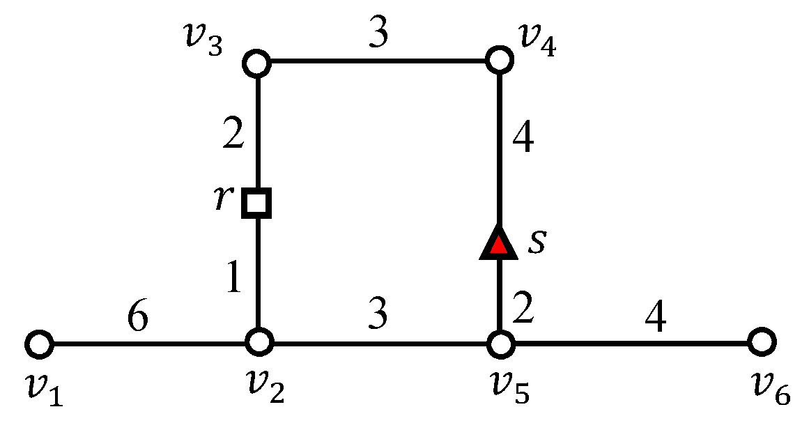
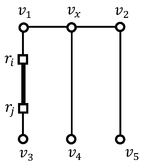
Figure 2 shows the difference between the distance and the segment length between two objects $r$ and $s$ in a road network, where the numbers at the edges indicate the distance between two adjacent points (e.g., $dist\left(v_1,v_2\right)=6$). The shortest path from $r$ to $s$ is denoted by $r\to v_2\to v_5\to s$ where the distance between $r$ and $s$ is $dist\left(r,s\right)=6$ in this case. The segment connecting $r$ and $s$ in the same vertex sequence $\overline{v_2{v}_3{v}_4{v}_5}$ becomes $\overline{r{v}_3{v}_{4}s}$ with length equal to $len\left(r,s\right)=9$. We recall that $len\left(r,s\right)$ is defined for two objects located in the same vertex sequence.

3.2. $\epsilon$-Distance Join Query

We consider two object sets $R$ and $S$ in the road network $G$. For convenience, $R$ is referred to as the set of outer objects and $S$ is referred to as the set of inner objects. Accordingly, $r\in R$ and $s\in S$ are referred to as outer and inner objects, respectively.

Definition 1.

($\epsilon$-distance join query): Given a threshold distance $\epsilon$ and two object sets $R$ and $S$, where $R=\left\{r_1,r_2,\cdots ,r_{\left|R\right|}\right\}$ and $S=\left\{s_1,s_2,\cdots ,s_{\left|S\right|}\right\}$, the $\epsilon$-distance join query, denoted by $R{\bowtie }_{\epsilon }S$, returns the set of all possible pairs of objects from $R\times S$ that are within the threshold distance $\epsilon$:

$$R{\bowtie }_{\epsilon }S=\left\{\left(r,s\right)|dist\left(r,s\right)\le \epsilon \mathrm{for} \forall \left(r,s\right)\in R\times S\right\}.$$

Naturally, $R{\bowtie }_{\epsilon }S$ is a subset of $R\times S$. The $\epsilon$-distance join query is commutative, i.e., $R{\bowtie }_{\epsilon }S=S{\bowtie }_{\epsilon }R$.

4. Naive Shared Execution for $\epsilon$-Distance Join Queries in Road Networks

4.1. Grouping of Objects in a Vertex Sequence

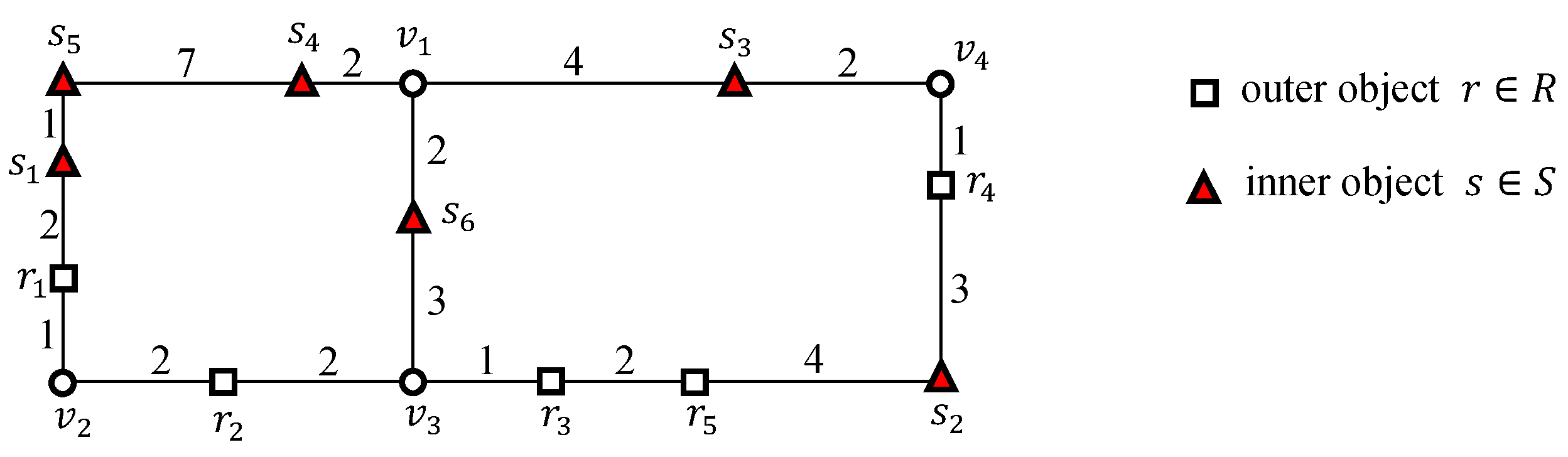
Figure 3 presents an example of an $\epsilon$-distance join query in a road network, which will be discussed throughout this section. In this figure, there are five outer objects, $r_1$ through $r_5$, and six inner objects, $s_1$ through $s_6$. Given a threshold distance $\epsilon =5$ and two object sets $R=\left\{r_1,r_2,r_3,r_4,r_5\right\}$ and $S=\left\{s_1,s_2,s_3,s_4,s_5,s_6\right\}$, we consider an $\epsilon$-distance join query $R{\bowtie }_{\epsilon }S$ of the following form: $R{\bowtie }_{\epsilon }S=\left\{\left(r,s\right)\right|dist\left(r,s\right)\le 5 \mathrm{for}\forall \left(r,s\right)\in R\times S\}$.

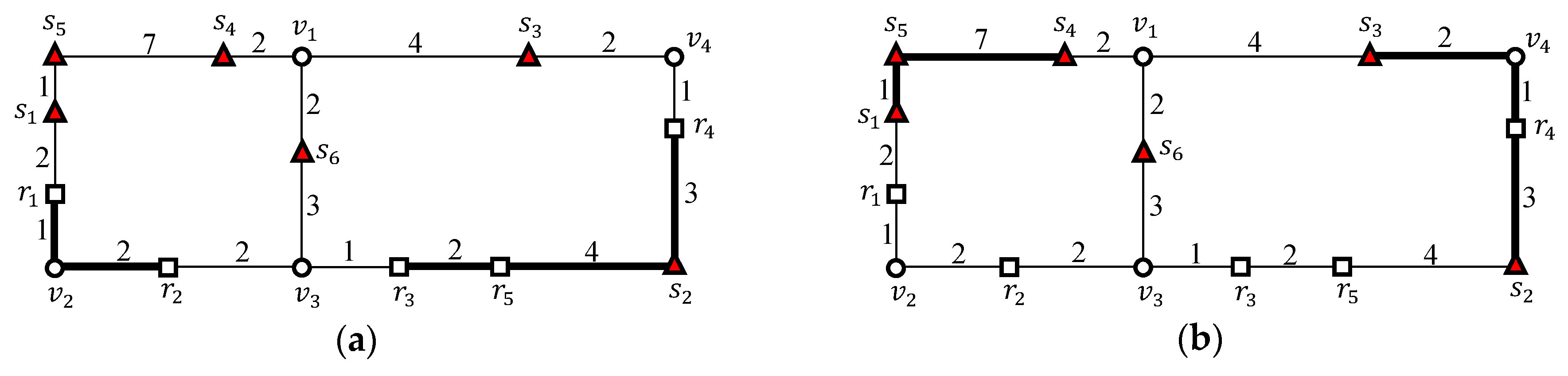
Figure 4 shows the sample grouping of outer objects in a vertex sequence and the sample grouping of inner objects in a vertex sequence. As shown in Figure 4a, two outer objects $r_1$ and $r_2$ in a vertex sequence $\overline{v_1{v}_2{v}_3}$ are grouped into an outer segment $\overline{r_1{r}_2}$, and three outer objects $r_3$, $r_4$, and $r_5$ in a vertex sequence $\overline{v_1{v}_4{v}_3}$ are grouped into another outer segment $\overline{r_3{r}_5{r}_4}$. Similarly, as shown in Figure 4b, three inner objects $s_1$, $s_4$, and $s_5$ in a vertex sequence $\overline{v_1{v}_2{v}_3}$ are grouped into an inner segment $\overline{s_1{s}_5{s}_4}$, and two inner objects $s_2$ and $s_3$ in a vertex sequence $\overline{v_1{v}_4{v}_3}$ are grouped into another inner segment $\overline{s_2{s}_3}$. Therefore, a set of outer objects $R=\left\{r_1,r_2,r_3,r_4,r_5\right\}$ is transformed into $\overline{R}=\left\{\overline{r_1{r}_2},\overline{r_3{r}_5{r}_4}\right\}$, where $\overline{R}$ is the set of outer segments generated from the outer objects. Similarly, a set of inner objects $S=\left\{s_1,s_2,s_3,s_4,s_5,s_6\right\}$ is transformed into $\overline{S}=\left\{\overline{s_1{s}_5{s}_4},\overline{s_2{s}_3},s_6\right\}$, where $\overline{S}$ is the set of inner segments generated from the inner objects. Without loss of generality, we assume that $\left|\overline{R}\right|\le \left|\overline{S}\right|$, because $R{\bowtie }_{\epsilon }S=S{\bowtie }_{\epsilon }R$. If $\left|\overline{R}\right|>\left|\overline{S}\right|$, then $S{\bowtie }_{\epsilon }R$ is evaluated instead of $R{\bowtie }_{\epsilon }S$.

4.2. Shared Execution Processing of Grouped Outer Objects

Our shared execution strategy for processing $\epsilon$-distance join queries in road networks is motivated by the observation that at most two range queries are sufficient for retrieving inner objects within the threshold distance $\epsilon$ from each outer object in an outer segment. This observation is formalized in Lemma 1, which states a simple but important fact regarding the shared execution of $\epsilon$-distance join queries in road networks—if we evaluate two range queries at outer objects $r_i$ and $r_j$, which correspond to the two end points of an outer segment $\overline{r_i{r}_{i+1}\dots r_j}$, then we can retrieve inner objects within distance $\epsilon$ from outer objects $r_{i+1},\cdots ,r_{j-1}$ without duplicating the network traversal. Thus, the two range queries at $r_i$ and $r_j$ are sufficient for retrieving inner objects within distance $\epsilon$ from the other outer objects $r_{i+1},\cdots ,r_{j-1}$.

Lemma 1.

For every outer object $r\in \overline{r_i{r}_j}$, it holds that $S_r^{\epsilon }\subseteq S_{r_i}^{\epsilon }{\displaystyle \cup }{S}_{r_j}^{\epsilon }{\displaystyle \cup }S\left(\overline{r_i{r}_j}\right)$, where $S_{r_i}^{\epsilon }$ ($S_{r_j}^{\epsilon }$) is the set of inner objects within distance $\epsilon$ from an outer object $r_i$ ($r_j$), and $S\left(\overline{r_i{r}_j}\right)$ is the set of inner objects located in the outer segment $\overline{r_i{r}_j}$ (e.g., $s_2\in \overline{r_3{r}_5{r}_4}$ in Figure 4).

Proof. 

We prove Lemma 1 by contradiction. We assume that $S_r^{\epsilon }\subseteq S_{r_i}^{\epsilon }{\displaystyle \cup }{S}_{r_j}^{\epsilon }{\displaystyle \cup }S\left(\overline{r_i{r}_j}\right)$ does not hold, i.e., $S_r^{\epsilon }⊈S_{r_i}^{\epsilon }{\displaystyle \cup }{S}_{r_j}^{\epsilon }{\displaystyle \cup }S\left(\overline{r_i{r}_j}\right)$. Then this implies that there is an inner object $s^{+} \in S_r^{\epsilon }$ such that $s^{+}\notin S_{r_i}^{\epsilon }{\displaystyle \cup }{S}_{r_j}^{\epsilon }{\displaystyle \cup }S\left(\overline{r_i{r}_j}\right)$, i.e., $s^{+}\notin S_{r_i}^{\epsilon }$, $s^{+}\notin S_{r_j}^{\epsilon }$, and $s^{+}\notin S\left(\overline{r_i{r}_j}\right)$. Clearly, $s^{+}\notin S_{r_i}^{\epsilon }$ means that $dist\left(r_i,s^{+}\right)>\epsilon$. Similarly, $s^{+}\notin S_{r_j}^{\epsilon }$ means that $dist\left(r_j,s^{+}\right)>\epsilon$. Clearly, $s^{+}\notin S\left(\overline{r_i{r}_j}\right)$ means that $s^{+}$ is not located in $\overline{r_i{r}_j}$. Therefore, the shortest path from $r$ to $s^{+}$ passes through either $r_i$ or $r_j$ and the distance from $r$ to $s^{+}$ is determined by $dist\left(r,s^{+}\right)=min\left\{len\left(r,r_i\right)+dist\left(r_i,s^{+}\right),len\left(r,r_j\right)+dist\left(r_j,s^{+}\right)\right\}$. From the previous condition, both $dist\left(r_i,s^{+}\right)>\epsilon$ and $dist\left(r_j,s^{+}\right)>\epsilon$, which leads to $dist\left(r,s^{+}\right)>\epsilon$. Thus, $s^{+}$ cannot belong to $S_r^{\epsilon }$, which contradicts the assumption that an inner object $s^{+}\in S_r^{\epsilon }$ exists such that $S_r^{\epsilon }⊈S_{r_i}^{\epsilon }{\displaystyle \cup }{S}_{r_j}^{\epsilon }{\displaystyle \cup }S\left(\overline{r_i{r}_j}\right)$. Consequently, it holds that $S_r^{\epsilon }\subseteq S_{r_i}^{\epsilon }{\displaystyle \cup }{S}_{r_j}^{\epsilon }{\displaystyle \cup }S\left(\overline{r_i{r}_j}\right)$ for $\forall r\in \overline{r_i{r}_j}$. □

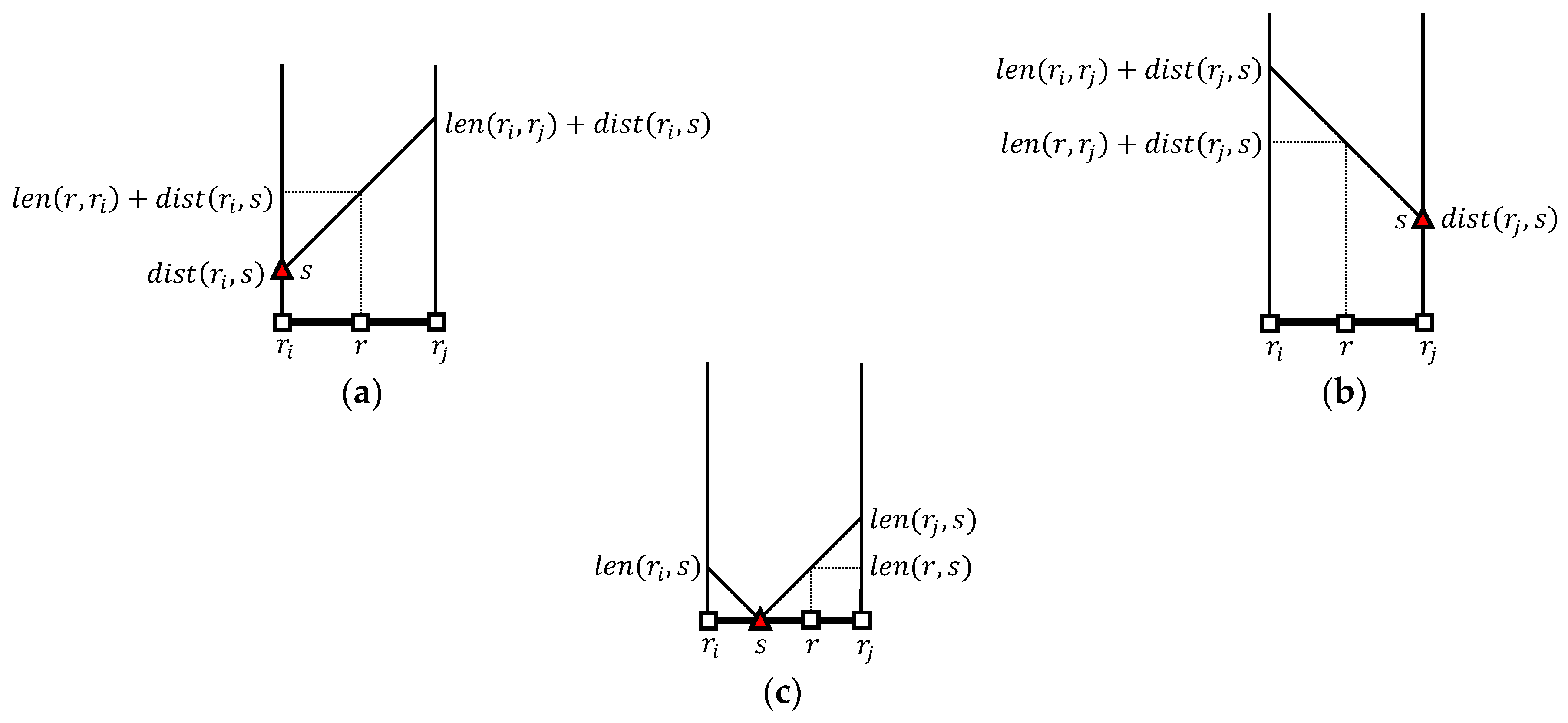
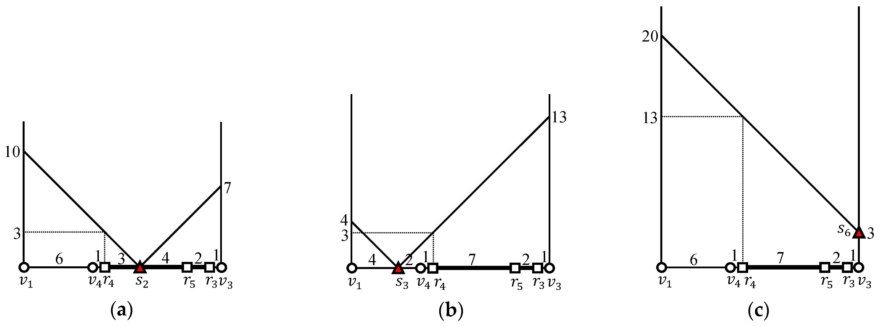
We determine the inner objects within distance $\epsilon$ from an outer object $r\in \overline{r_i{r}_j}$ among inner objects in $S_{r_i}^{\epsilon }{\displaystyle \cup }{S}_{r_j}^{\epsilon }{\displaystyle \cup }S\left(\overline{r_i{r}_j}\right)$. First, we compute the distance from an outer object $r\in \overline{r_i{r}_j}$ to an inner object $s\in S_{r_i}^{\epsilon }{\displaystyle \cup }{S}_{r_j}^{\epsilon }{\displaystyle \cup }S\left(\overline{r_i{r}_j}\right)$. If there exists a path $r\to r_i\to s$ (i.e., $s\in S_{r_i}^{\epsilon }$), then the distance from $r$ to $s$ is $dist\left(r,s\right)=len\left(r,r_i\right)+dist\left(r_i,s\right)$, as shown in Figure 5a. Similarly, if there exists a path $r\to r_j\to s$ (i.e., $s\in S_{r_j}^{\epsilon }$), then the distance from $r$ to $s$ is $dist\left(r,s\right)=len\left(r,r_j\right)+dist\left(r_j,s\right)$, as shown in Figure 5b. If the inner object $s$ is located in $\overline{r_i{r}_j}$ (i.e., $s\in \overline{r_i{r}_j}$), then the distance from $r$ to $s$ is $dist\left(r,s\right)=len\left(r,s\right)$, as shown in Figure 5c. Because $dist\left(r,s\right)$ is the length of the shortest path among multiple paths between $r$ and $s$, $dist\left(r,s\right)$ is computed as follows.

$$dist\left(r,s\right)=\{\begin{array}{ll}min\left\{len\left(r,r_i\right)+dist\left(r_i,s\right),len\left(r,r_j\right)+dist\left(r_j,s\right)\right\}\hfill & \mathrm{if}s\notin \overline{r_i{r}_j}\hfill \\ min\left\{len\left(r,r_i\right)+dist\left(r_i,s\right),len\left(r,r_j\right)+dist\left(r_j,s\right),len\left(r,s\right)\right\}\hfill & \mathrm{otherwise}\hfill \end{array}$$

Table 2. Computation of $dist\left(r,s\right)$ for $r\in \overline{r_i{r}_j}$ and $s\in S_{r_i}^{\epsilon }{\displaystyle \cup }{S}_{r_j}^{\epsilon }{\displaystyle \cup }S\left(\overline{r_i{r}_j}\right)$.

Condition	$\mathit{d}\mathit{i}\mathit{s}\mathit{t}\left(\mathit{r},\mathit{s}\right)$
$s\in S_{r_i}^{\epsilon }{\displaystyle \cap }{S}_{r_j}^{\epsilon }{\displaystyle \cap }S\left(\overline{r_i{r}_j}\right)$	$dist\left(r,s\right)=min\left\{len\left(r,r_i\right)+dist\left(r_i,s\right),len\left(r,r_j\right)+dist\left(r_j,s\right),len\left(r,s\right)\right\}$
$s\in S_{r_i}^{\epsilon }{\displaystyle \cap }{S}_{r_j}^{\epsilon }-S\left(\overline{r_i{r}_j}\right)$	$dist\left(r,s\right)=min\left\{len\left(r,r_i\right)+dist\left(r_i,s\right),len\left(r,r_j\right)+dist\left(r_j,s\right)\right\}$
$s\in S_{r_i}^{\epsilon }{\displaystyle \cap }S\left(\overline{r_i{r}_j}\right)-S_{r_j}^{\epsilon }$	$dist\left(r,s\right)=min\left\{len\left(r,r_i\right)+dist\left(r_i,s\right),len\left(r,s\right)\right\}$
$s\in S_{r_j}^{\epsilon }{\displaystyle \cap }S\left(\overline{r_i{r}_j}\right)-S_{r_i}^{\epsilon }$	$dist\left(r,s\right)=min\left\{len\left(r,r_j\right)+dist\left(r_j,s\right),len\left(r,s\right)\right\}$
$s\in S_{r_i}^{\epsilon }-\left(S_{r_j}^{\epsilon }{\displaystyle \cup }S\left(\overline{r_i{r}_j}\right)\right)$	$dist\left(r,s\right)=len\left(r,r_i\right)+dist\left(r_i,s\right)$
$s\in S_{r_j}^{\epsilon }-\left(S_{r_i}^{\epsilon }{\displaystyle \cup }S\left(\overline{r_i{r}_j}\right)\right)$	$dist\left(r,s\right)=len\left(r,r_j\right)+dist\left(r_j,s\right)$
$s\in S\left(\overline{r_i{r}_j}\right)-\left(S_{r_i}^{\epsilon }{\displaystyle \cup }{S}_{r_j}^{\epsilon }\right)$	$dist\left(r,s\right)=len\left(r,s\right)$

explains how to compute the distance from $r$ to $s$, where $r\in \overline{r_i{r}_j}$ and $s\in S_{r_i}^{\epsilon }{\displaystyle \cup }{S}_{r_j}^{\epsilon }{\displaystyle \cup }S\left(\overline{r_i{r}_j}\right)$. The inner object $s$ belongs to a combination of $S_{r_i}^{\epsilon }$, $S_{r_j}^{\epsilon }$, and $S\left(\overline{r_i{r}_j}\right)$, so seven possible cases are considered in total. Clearly, it is trivial to retrieve a set $S\left(\overline{r_i{r}_j}\right)$ of inner objects that are located in $\overline{r_i{r}_j}$ compared with retrieving a set $S_{r_i}^{\epsilon }$ ($S_{r_j}^{\epsilon }$) of inner objects within distance $\epsilon$ from an outer object $r_i$ ($r_j$).

4.3. Naive EDISON Algorithm

Algorithm 1 describes the naive EDISON algorithm, which employs the grouping of outer objects and shared execution to reduce query processing time. This algorithm involves two steps. In the first step, adjacent outer objects in a vertex sequence are grouped into an outer segment. Similarly, adjacent inner objects in a vertex sequence are also grouped into an inner segment. In other words, $R$ and $S$ are transformed into $\overline{R}$ and $\overline{S}$, respectively. For simplicity, we assume that $\left|\overline{R}\right|\le \left|\overline{S}\right|$. If $\left|\overline{R}\right|>\left|\overline{S}\right|$, we simply evaluate $S{\bowtie }_{\epsilon }R$, because $R{\bowtie }_{\epsilon }S=S{\bowtie }_{\epsilon }R$. In the second step, the naive EDISON algorithm explores each outer segment $\overline{r_i{r}_j}$ sequentially to retrieve inner objects that are within distance $\epsilon$ from each outer object in the outer segment $\overline{r_i{r}_j}$. Depending on the number of outer objects in $\overline{r_i{r}_j}$, there are three possible cases, which the naive EDISON algorithm handles differently: (1) $\left|\overline{r_i{r}_j}\right|=1$; (2) $\left|\overline{r_i{r}_j}\right|=2$; and (3) $\left|\overline{r_i{r}_j}\right|>2$. If $\left|\overline{r_i{r}_j}\right|=1$, a range query $RNQ\left(\epsilon ,r_i\right)$ is evaluated at $r_i$ because $\overline{r_i{r}_j}$ includes an outer object $r_i$ ($=r_j$) only. Then, a partial join result $\mathsf{\Phi }\left(r_i\right)$ is simply obtained from the range query result $S_{r_i}^{\epsilon }$ at $r_i$, i.e., $\mathsf{\Phi }\left(r_i\right)=\left\{\left(r_i,s\right)\right|s\in S_{r_i}^{\epsilon }\}$. The partial join result $\mathsf{\Phi }\left(r_i\right)$ is added to the $\epsilon$-distance join query result $\mathsf{\Phi }\left(R\right)$, i.e., $\mathsf{\Phi }\left(R\right)=\mathsf{\Phi }\left(R\right){\displaystyle \cup }\mathsf{\Phi }\left(r_i\right)$ (lines 8‒10). If $\left|\overline{r_i{r}_j}\right|=2$, two range queries, $RNQ\left(\epsilon ,r_i\right)$ and $RNQ\left(\epsilon ,r_j\right)$, are evaluated at $r_i$ and $r_j$, respectively, because $\overline{r_i{r}_j}$ includes only two outer objects $r_i$ and $r_j$. Then, two partial join results $\mathsf{\Phi }\left(r_i\right)$ and $\mathsf{\Phi }\left(r_j\right)$ are simply obtained from the range query results $S_{r_i}^{\epsilon }$ and $S_{r_j}^{\epsilon }$ at $r_i$ and $r_j$, respectively, i.e., $\mathsf{\Phi }\left(r_i\right)=\left\{\left(r_i,s\right)\right|s\in S_{r_i}^{\epsilon }\}$ and $\mathsf{\Phi }\left(r_j\right)=\left\{\left(r_j,s\right)\right|s\in S_{r_j}^{\epsilon }\}$. These partial join results $\mathsf{\Phi }\left(r_i\right)$ and $\mathsf{\Phi }\left(r_j\right)$ are added to the $\epsilon$-distance join query result $\mathsf{\Phi }\left(R\right)$, i.e., $\mathsf{\Phi }\left(R\right)=\mathsf{\Phi }\left(R\right){\displaystyle \cup }\mathsf{\Phi }\left(r_i\right){\displaystyle \cup }\mathsf{\Phi }\left(r_j\right)$ (lines 11‒14). Finally, if $\left|\overline{r_i{r}_j}\right|>2$, only two range queries, $RNQ\left(\epsilon ,r_i\right)$ and $RNQ\left(\epsilon ,r_j\right)$, are evaluated at $r_i$ and $r_j$, respectively, similar to the case of $\left|\overline{r_i{r}_j}\right|=2$. According to Lemma 1, a partial join result $\mathsf{\Phi }\left(\overline{r_i{r}_j}\right)$ can be obtained from $S_{r_i}^{\epsilon }{\displaystyle \cup }{S}_{r_j}^{\epsilon }{\displaystyle \cup }S\left(\overline{r_i{r}_j}\right)$ using the shared execution method (lines 15‒19), which is detailed in Lemma 2. This is because the partial join result $\mathsf{\Phi }\left(\overline{r_i{r}_j}\right)$ is the set of object pairs $\left(r,s\right)$ that are within distance $\epsilon$, where $r\in \overline{r_i{r}_j}$ and $s\in S_{r_i}^{\epsilon }{\displaystyle \cup }{S}_{r_j}^{\epsilon }{\displaystyle \cup }S\left(\overline{r_i{r}_j}\right)$, i.e., $\mathsf{\Phi }\left(\overline{r_i{r}_j}\right)=\left\{\left(r,s\right)\right|dist\left(r,s\right)\le \epsilon \mathrm{for}r\in \overline{r_i{r}_j} \mathrm{and} s\in S_{r_i}^{\epsilon }{\displaystyle \cup }{S}_{r_j}^{\epsilon }{\displaystyle \cup }S\left(\overline{r_i{r}_j}\right)\}$. Finally, the $\epsilon$-distance join query result $\mathsf{\Phi }\left(R\right)$ is returned after all outer segments have been processed (line 20), i.e., $\mathsf{\Phi }\left(R\right)={\displaystyle \bigcup }\mathsf{\Phi }\left(\overline{r_i{r}_j}\right)$ for each outer segment $\overline{r_i{r}_j}\in \overline{R}$. In Lemma 2, we prove the correctness of the naive EDISON algorithm.

Algorithm 1: Naive_EDISON ($\epsilon ,R,S$)
Input:$\epsilon$: threshold distance, $R$: set of outer objects, $S$: set of inner objects
Output:$R{\bowtie }_{\epsilon }S$: set of object pairs $\left(r,s\right)\in R\times S$ such that $dist\left(r,s\right)\le \epsilon$
1	$\mathsf{\Phi }\left(R\right)\leftarrow \varnothing$			// $\mathsf{\Phi }\left(R\right)$ is the set of object pairs $\left(r,s\right)\in R\times S$ such that $dist\left(r,s\right)\le \epsilon$.
2	// Step 1: neighboring outer objects are grouped and neighboring inner objects are also grouped.
3	$\overline{R}\leftarrow group\_objects\left(R\right)$			// Outer objects in a vertex sequence are grouped into an outer segment.
4	$\overline{S}\leftarrow group\_objects\left(S\right)$			// Inner objects in a vertex sequence are grouped into an inner segment.
5	// For simplicity, we assume that $\left|\overline{R}\right|\le \left|\overline{S}\right|$. if $\left|\overline{R}\right|>\left|\overline{S}\right|$, we simply evaluate $S{\bowtie }_{\epsilon }R$.
6	// Step 2: $\overline{r_i{r}_j}{\bowtie }_{\epsilon }S$ is evaluated for each outer segment $\overline{r_i{r}_j}\in \overline{R}$.
7	for each outer segment $\overline{r_i{r}_j}\in \overline{R}$ do
8		if$\left|\overline{r_i{r}_j}\right|=1$then		// $\left|\overline{r_i{r}_j}\right|=1$ means that $\overline{r_i{r}_j}$ contains an outer object $r_i$ only.
9			$S_{r_i}^{\epsilon }\leftarrow RNQ\left(\epsilon ,r_i\right)$	// A range query is evaluated at $r_i$ and its result is $S_{r_i}^{\epsilon }$.
10			$\mathsf{\Phi }\left(R\right)\leftarrow \mathsf{\Phi }\left(R\right){\displaystyle \cup }\mathsf{\Phi }\left(r_i\right)$	// Note that $\mathsf{\Phi }\left(r_i\right)=\left\{\left(r_i,s\right)\right|s\in S_{r_i}^{\epsilon }\}$.
11		else if$\left|\overline{r_i{r}_j}\right|=2$then		//$\left|\overline{r_i{r}_j}\right|=2$ means that $\overline{r_i{r}_j}$ contains two outer objects $r_i$ and $r_j$.
12			$S_{r_i}^{\epsilon }\leftarrow RNQ\left(\epsilon ,r_i\right)$	// A range query is evaluated at $r_i$ and its result is $S_{r_i}^{\epsilon }$.
13			$S_{r_j}^{\epsilon }\leftarrow RNQ\left(\epsilon ,r_j\right)$	// Another range query is evaluated at $r_j$ and its result is $S_{r_j}^{\epsilon }$.
14			$\mathsf{\Phi }\left(R\right)\leftarrow \mathsf{\Phi }\left(R\right){\displaystyle \cup }\mathsf{\Phi }\left(r_i\right){\displaystyle \cup }\mathsf{\Phi }\left(r_j\right)$	// Note that $\mathsf{\Phi }\left(r_i\right)=\left\{\left(r_i,s\right)\right|s\in S_{r_i}^{\epsilon }\}$ and $\mathsf{\Phi }\left(r_j\right)=\left\{\left(r_j,s\right)\right|s\in S_{r_j}^{\epsilon }\}$.
15		else if$\left|\overline{r_i{r}_j}\right|>2$then		// $\left|\overline{r_i{r}_j}\right|\ge 2$ means that $\overline{r_i{r}_j}$ contains more than two outer objects.
16			$S_{r_i}^{\epsilon }\leftarrow RNQ\left(\epsilon ,r_i\right)$	// A range query is evaluated at $r_i$ and its result is $S_{r_i}^{\epsilon }$.
17			$S_{r_j}^{\epsilon }\leftarrow RNQ\left(\epsilon ,r_j\right)$	// Another range query is evaluated at $r_j$ and its result is $S_{r_j}^{\epsilon }$.
18			$\mathsf{\Phi }\left(\overline{r_i{r}_j}\right)\leftarrow DJQ\left(\epsilon ,\overline{r_i{r}_j}, S_{r_i}^{\epsilon }{\displaystyle \cup }{S}_{r_j}^{\epsilon }{\displaystyle \cup }S\left(\overline{r_i{r}_j}\right)\right)$	// $DJQ$ is explained in Algorithm 3.
19			$\mathsf{\Phi }\left(R\right)\leftarrow \mathsf{\Phi }\left(R\right){\displaystyle \cup }\mathsf{\Phi }\left(\overline{r_i{r}_j}\right)$	// $\mathsf{\Phi }\left(\overline{r_i{r}_j}\right)=\left\{\left(r,s\right)\right|dist\left(r,s\right)\le \epsilon \mathrm{for}r\in \overline{r_i{r}_j}, s\in S_{r_i}^{\epsilon }{\displaystyle \cup }{S}_{r_j}^{\epsilon }{\displaystyle \cup }S\left(\overline{r_i{r}_j}\right)\}$.
20	return$\mathsf{\Phi }\left(R\right)$			// $\mathsf{\Phi }\left(R\right)$ stores the result of $R{\bowtie }_{\epsilon }S$.

Lemma 2.

The naive EDISON algorithm is correct.

Proof. 

We prove the correctness of the naive EDISON algorithm by cases. As shown in Algorithm 1, the naive EDISON algorithm handles the following three cases differently depending on the number of outer objects in an outer segment $\overline{r_i{r}_j}$, namely, (1) $\left|\overline{r_i{r}_j}\right|=1$, (2) $\left|\overline{r_i{r}_j}\right|=2$, and (3) $\left|\overline{r_i{r}_j}\right|>2$. In the first two cases (i.e., $\left|\overline{r_i{r}_j}\right|=1$ and $\left|\overline{r_i{r}_j}\right|=2$), a range query is used to retrieve inner objects $s$ within distance $\epsilon$ from each outer object $r\in \overline{r_i{r}_j}$. This is same as a straightforward method used to answer $\epsilon$-distance join queries by issuing a range query for each outer object $r\in R$. For $\left|\overline{r_i{r}_j}\right|=1$, the naive EDISON algorithm evaluates a range query $RNQ\left(\epsilon ,r_i\right)$ for only an outer object $r_i$, and adds an object pair $\left(r_i,s\right)$ to the $\epsilon$-distance join query result for each inner object $s\in S_{r_i}^{\epsilon }$. Therefore, the naive EDISON algorithm is correct for $\left|\overline{r_i{r}_j}\right|=1$ because $RNQ\left(\epsilon ,r_i\right)$ simply retrieves inner objects $s$ within distance $\epsilon$ from $r_i$. Similarly, for $\left|\overline{r_i{r}_j}\right|=2$, the naive EDISON algorithm evaluates two range queries, $RNQ\left(\epsilon ,r_i\right)$ and $RNQ\left(\epsilon ,r_j\right)$, for two outer objects $r_i$ and $r_j$, respectively. The naive EDISON algorithm then adds an object pair $\left(r_i,s\right)$ to the $\epsilon$-distance join query result for each inner object $s\in S_{r_i}^{\epsilon }$, and adds an object pair $\left(r_j,s\right)$ to the $\epsilon$-distance join query result for each inner object $s\in S_{r_j}^{\epsilon }$. Therefore, the naive EDISON algorithm is correct for $\left|\overline{r_i{r}_j}\right|=2$ because $RNQ\left(\epsilon ,r_i\right)$ and $RNQ\left(\epsilon ,r_j\right)$ retrieve inner objects $s$ within distance $\epsilon$ from $r_i$ and $r_j$, respectively.

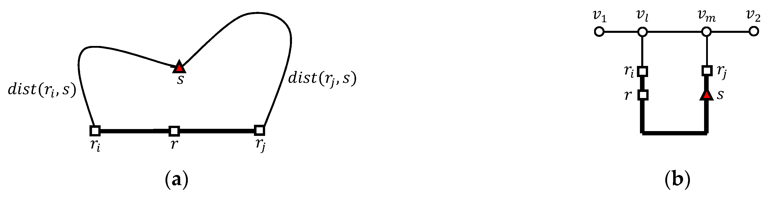
The proof for the correctness of the naive EDISON algorithm for $\left|\overline{r_i{r}_j}\right|>2$ differs from that for $\left|\overline{r_i{r}_j}\right|=1$ and $\left|\overline{r_i{r}_j}\right|=2$ because the naive EDISON algorithm exploits the shared execution strategy for $\left|\overline{r_i{r}_j}\right|>2$. Note that the naive EDISON algorithm evaluates only two range queries $RNQ\left(\epsilon ,r_i\right)$ and $RNQ\left(\epsilon ,r_j\right)$ for $\left|\overline{r_i{r}_j}\right|>2$. The key idea of the proof of the correctness for $\left|\overline{r_i{r}_j}\right|>2$ is to compute the distance between an outer object $r$ and each candidate inner object $s$ without evaluating a range query for $r$, where $r\in \overline{r_i{r}_j}-\left\{r_i,r_j\right\}$ and $s\in S_{r_i}^{\epsilon }{\displaystyle \cup }{S}_{r_j}^{\epsilon }{\displaystyle \cup }S\left(\overline{r_i{r}_j}\right)$. According to Lemma 1, we can retrieve inner objects within distance $\epsilon$ from every outer object $r\in \overline{r_i{r}_j}$ among the candidate inner objects $s\in S_{r_i}^{\epsilon }{\displaystyle \cup }{S}_{r_j}^{\epsilon }{\displaystyle \cup }S\left(\overline{r_i{r}_j}\right)$. The distance between $r$ and $s$, $dist\left(r,s\right)$, determines whether an object pair $\left(r,s\right)$ is included in the $\epsilon$-distance join query result. Let us compute the distance between an outer object $r$ and candidate inner object $s$. To do so, we consider the two cases, $s\notin \overline{r_i{r}_j}$ and $s\in \overline{r_i{r}_j}$, as shown in Figure 6a,b, respectively. If $s\notin \overline{r_i{r}_j}$, the distance from $r$ to $s$ is evaluated as $dist\left(r,s\right)=min\left\{len\left(r,r_i\right)+dist\left(r_i,s\right),len\left(r,r_j\right)+dist\left(r_j,s\right)\right\}$ because there are two possible paths from $r$ to $s$, i.e., $r\to r_i\to s$ and $r\to r_j\to s$; otherwise, the distance from $r$ to $s$ is evaluated as $dist\left(r,s\right)=min\left\{len\left(r,r_i\right)+dist\left(r_i,s\right),len\left(r,r_j\right)+dist\left(r_j,s\right),len\left(r,s\right)\right\}$ because there are three possible paths from $r$ to $s$, i.e., $r\to r_i\to s$, $r\to r_j\to s$, and $r\to s$. If $dist\left(r,s\right)\le \epsilon$, an object pair $\left(r,s\right)$ is included in the $\epsilon$-distance join query result; otherwise, the object pair $\left(r,s\right)$ is not included. Therefore, the naive EDISON algorithm is correct for $\left|\overline{r_i{r}_j}\right|>2$. Consequently, the naive EDISON algorithm is correct for $\left|\overline{r_i{r}_j}\right|=1$, $\left|\overline{r_i{r}_j}\right|=2$, and $\left|\overline{r_i{r}_j}\right|>2$. □

4.4. Evaluation of an Example $\epsilon$-Distance Join Query Using the Naive EDISON Algorithm

We discuss how to evaluate the $\epsilon$-distance join query in Figure 3 using the naive EDISON algorithm. Recall that $\epsilon =5$, $R=\left\{r_1,r_2,r_3,r_4,r_5\right\}$, and $S=\left\{s_1,s_2,s_3,s_4,s_5,s_6\right\}$ are given and that outer objects $r_1$ through $r_5$ are grouped into outer segments $\overline{r_1{r}_2}$ and $\overline{r_3{r}_5{r}_4}$, as shown in Figure 4.

Table 3. Computation of $R{\bowtie }_{\epsilon }S$ using the naive EDISON algorithm.

$\overline{{\mathit{r}}_{\mathit{i}}{\mathit{r}}_{\mathit{j}}}$	${\mathit{r}}_{\mathit{i}}$	${\mathit{r}}_{\mathit{j}}$	${\mathit{S}}_{{\mathit{r}}_{\mathit{i}}}^{\mathit{\epsilon }}$	${\mathit{S}}_{{\mathit{r}}_{\mathit{j}}}^{\mathit{\epsilon }}$	$\mathit{S}\left(\overline{{\mathit{r}}_{\mathit{i}}{\mathit{r}}_{\mathit{j}}}\right)$	$\left\{{\mathit{r}}_{\mathit{i}+1},\dots ,{\mathit{r}}_{\mathit{j}-1}\right\}$	${\mathit{S}}_{{\mathit{r}}_{\mathit{i}}}^{\mathit{\epsilon }}{\displaystyle \cup }{\mathit{S}}_{{\mathit{r}}_{\mathit{j}}}^{\mathit{\epsilon }}{\displaystyle \cup }\mathit{S}\left(\overline{{\mathit{r}}_{\mathit{i}}{\mathit{r}}_{\mathit{j}}}\right)$
$\overline{r_1{r}_2}$	$r_1$	$r_2$	$S_{r_1}^{\epsilon }=\left\{s_1,s_5\right\}$	$S_{r_2}^{\epsilon }=\left\{s_1,s_6\right\}$	$S\left(\overline{r_1{r}_2}\right)=\varnothing$	$\varnothing$	$\left\{s_1,s_5,s_6\right\}$
$\overline{r_3{r}_5{r}_4}$	$r_3$	$r_4$	$S_{r_3}^{\epsilon }=\left\{s_6\right\}$	$S_{r_4}^{\epsilon }=\left\{s_2,s_3\right\}$	$S\left(\overline{r_3{r}_5{r}_4}\right)=\left\{s_2\right\}$	$\left\{r_5\right\}$	$\left\{s_2,s_3,s_6\right\}$

summarizes the computation of $R{\bowtie }_{\epsilon }S$ for the naive EDISON algorithm.

Because Algorithm 1 processes outer segments one by one, we determine inner objects within the threshold distance $\epsilon$ from each outer object $r\in \overline{r_1{r}_2}$ followed by $\overline{r_3{r}_5{r}_4}$. Two range queries $RNQ\left(5,r_1\right)$ and $RNQ\left(5,r_2\right)$ are evaluated for an outer segment $\overline{r_1{r}_2}$, whose results are $S_{r_1}^{\epsilon }=\left\{s_1,s_5\right\}$ and $S_{r_2}^{\epsilon }=\left\{s_1,s_6\right\}$, respectively. Because $\left|\overline{r_1{r}_2}\right|=2$ holds, we can simply obtain the partial join result $\mathsf{\Phi }\left(\overline{r_1{r}_2}\right)$ for $\overline{r_1{r}_2}$, i.e., $\mathsf{\Phi }\left(\overline{r_1{r}_2}\right)=\mathsf{\Phi }\left(r_1\right){\displaystyle \cup }\mathsf{\Phi }\left(r_2\right)=\left\{\left(r_1,s_1\right),\left(r_1,s_5\right),\left(r_2,s_1\right),\left(r_2,s_6\right)\right\}$.

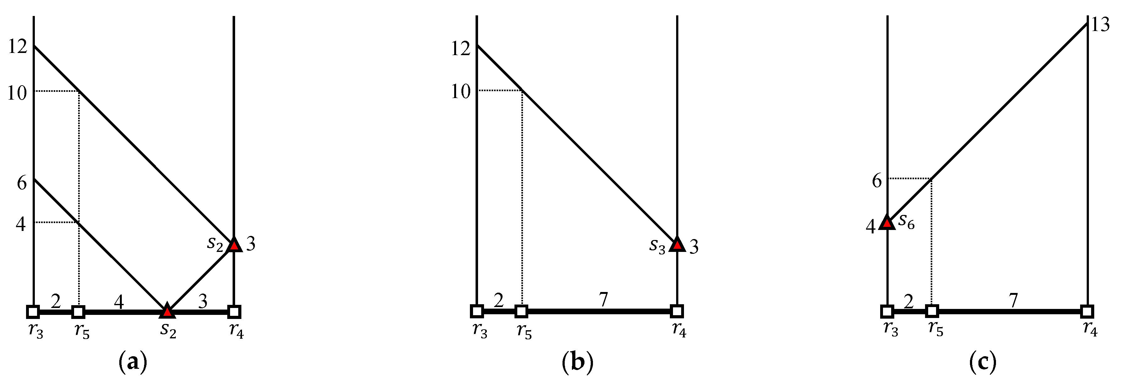
Similarly, two range queries $RNQ\left(5,r_3\right)$ and $RNQ\left(5,r_4\right)$ are evaluated for an outer segment $\overline{r_3{r}_5{r}_4}$, whose results are $S_{r_3}^{\epsilon }=\left\{s_6\right\}$ and $S_{r_4}^{\epsilon }=\left\{s_2,s_3\right\}$, respectively. Because we have $S_{r_3}^{\epsilon }=\left\{s_6\right\}$, $S_{r_4}^{\epsilon }=\left\{s_2,s_3\right\}$, and $S\left(\overline{r_3{r}_5{r}_4}\right)=\left\{s_2\right\}$, we can compute the distance $\epsilon$ from $r_5\in \overline{r_3{r}_5{r}_4}$ to each candidate inner object $s\in S_{r_3}^{\epsilon }{\displaystyle \cup }{S}_{r_4}^{\epsilon }{\displaystyle \cup }S\left(\overline{r_3{r}_5{r}_4}\right)$ and can retrieve inner objects within distance $\epsilon$ from $r_5$. For this, we need to compute the distance from $r_5$ to each candidate inner object $s\in \left\{s_2,s_3,s_6\right\}$. Because $s_2\in S_{r_4}^{\epsilon }{\displaystyle \cap }S\left(\overline{r_3{r}_5{r}_4}\right)-S_{r_3}^{\epsilon }$ according to Table 3, the distance from $r_5$ to $s_2$ is $dist\left(r_5,s_2\right)=min\left\{len\left(r_5,r_4\right)+dist\left(r_4,s_2\right),len\left(r_5,s_2\right)\right\}=\min \left\{10,4\right\}=4$, as shown in Figure 7a. Similarly, because $s_3\in S_{r_4}^{\epsilon }-\left(S_{r_3}^{\epsilon }{\displaystyle \cup }S\left(\overline{r_3{r}_5{r}_4}\right)\right)$ according to Table 3, the distance from $r_5$ to $s_3$ is $dist\left(r_5,s_3\right)=len\left(r_5,r_4\right)+dist\left(r_4,s_3\right)=10$, as shown in Figure 7b. Finally, because $s_6\in S_{r_3}^{\epsilon }-\left(S_{r_4}^{\epsilon }{\displaystyle \cup }S\left(\overline{r_1{r}_5{r}_4}\right)\right)$ according to Table 3, the distance from $r_5$ to $s_6$ is $dist\left(r_5,s_6\right)=len\left(r_5,r_3\right)+dist\left(r_3,s_6\right)=6$, as shown in Figure 7c. Thus, $S_{r_5}^{\epsilon }=\left\{s_2\right\}$ given that $dist\left(r_5,s_2\right)=4$, $dist\left(r_5,s_3\right)=10$, and $dist\left(r_5,s_6\right)=6$. The partial join result $\mathsf{\Phi }\left(\overline{r_3{r}_5{r}_4}\right)$ for $\overline{r_3{r}_5{r}_4}$ is obtained by taking the union of the three range query results at $r_3$, $r_4$, and $r_5$, i.e., $\mathsf{\Phi }\left(\overline{r_3{r}_5{r}_4}\right)=\mathsf{\Phi }\left(r_3\right){\displaystyle \cup }\mathsf{\Phi }\left(r_4\right){\displaystyle \cup }\mathsf{\Phi }\left(r_5\right)=\left\{\left(r_3,s_6\right),\left(r_4,s_2\right),\left(r_4,s_3\right),\left(r_5,s_2\right)\right\}$ where $\mathsf{\Phi }\left(r_3\right)=\left\{\left(r_3,s_6\right)\right\}$, $\mathsf{\Phi }\left(r_4\right)=\left\{\left(r_4,s_2\right),\left(r_4,s_3\right)\right\}$, and $\mathsf{\Phi }\left(r_5\right)=\left\{\left(r_5,s_2\right)\right\}$. Consequently, we have the result $\mathsf{\Phi }\left(R\right)$ of the $\epsilon$-distance join query, i.e., $\mathsf{\Phi }\left(R\right)=\mathsf{\Phi }\left(\overline{r_1{r}_2}\right){\displaystyle \cup }\mathsf{\Phi }\left(\overline{r_3{r}_5{r}_4}\right)=\left\{\left(r_1,s_1\right),\left(r_1,s_5\right),\left(r_2,s_1\right),\left(r_2,s_6\right),\left(r_3,s_6\right),\left(r_4,s_2\right),\left(r_4,s_3\right),\left(r_5,s_2\right)\right\}$.

5. Optimal Shared Execution for $\epsilon$-Distance Join Queries in Road Networks

5.1. Extending Shared Execution Processing to Adjacent Outer Segments

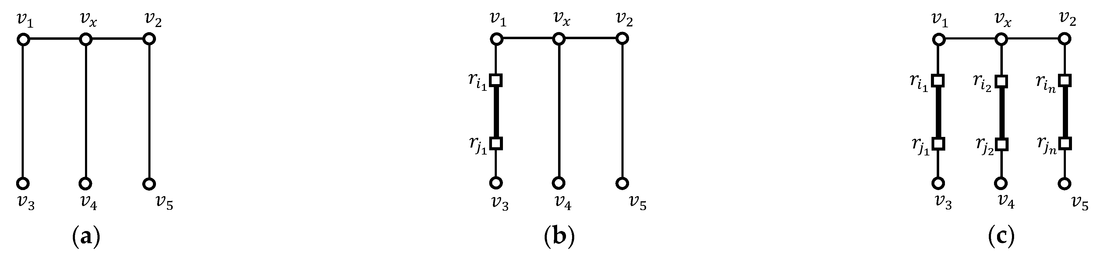
We can extend the shared execution processing to adjacent outer segments. We call this shared execution processing the EDISON method. To this end, we investigate the number of outer segments that belong to adjacent vertex sequences of an intersection vertex. Let $\mathsf{\Omega }\left(v_x\right)$ be the number of outer segments in vertex sequences adjacent to an intersection vertex $v_x$. If $\mathsf{\Omega }\left(v_x\right)=0$, as shown in Figure 8a, no range query is issued at $v_x$. If $\mathsf{\Omega }\left(v_x\right)=1$, as shown in Figure 8b, a range query $RNQ\left(\epsilon ,r_i\right)$ is issued at $r_i$. If $\mathsf{\Omega }\left(v_x\right)\ge 2$, as shown in Figure 8c, a range query $RNQ\left({\epsilon }_{v_x},v_x\right)$ is issued at $v_x$, where $\mathsf{\Omega }\left(v_x\right)=n$ and ${\epsilon }_{v_x}=\epsilon -min\left\{len\left(v_x,r_{i_1}\right),len\left(v_x,r_{i_2}\right),\cdots ,len\left(v_x,r_{i_n}\right)\right\}$. Naturally, if ${\epsilon }_{v_x}\le 0$, no range query at $v_x$ is issued. In summary, if $\mathsf{\Omega }\left(v_x\right)=1$, the same shared execution as the naive EDISON algorithm is applied to an outer segment, and if $\mathsf{\Omega }\left(v_x\right)\ge 2$, an extended shared execution is applied to outer segments adjacent to $v_x$.

Returning to the example in Figure 3, we reevaluate the $\epsilon$-distance join query to demonstrate the effectiveness of considering the shared execution of adjacent outer segments. To answer the $\epsilon$-distance join query, the naive EDISON method would evaluate four range queries $RNQ\left(5,r_1\right)$, $RNQ\left(5,r_2\right)$,$RNQ\left(5,r_3\right)$, and $RNQ\left(5,r_4\right)$ whereas the EDISON method only evaluates the range query $RNQ\left(4,v_3\right)$ at the intersection vertex $v_3$. This occurs because there are two intersection vertices $v_1$ and $v_3$, as shown in Figure 4a and we have $\mathsf{\Omega }\left(v_1\right)=2$, $\mathsf{\Omega }\left(v_3\right)=2$, ${\epsilon }_{v_1}=\epsilon -min\left\{len\left(v_1,r_1\right),len\left(v_1,r_4\right)\right\}=5-min\left\{12,7\right\}=-2$, so ${\epsilon }_{v_3}=\epsilon -min\left\{len\left(v_3,r_2\right),len\left(v_3,r_3\right)\right\}=5-min\left\{2,1\right\}=4$.

We present a simple heuristic where no range queries close to terminal vertices are issued. As shown in Figure 9, the example network has one intersection vertex $v_x$ and three terminal vertices $v_3$, $v_4$, and $v_5$. In this figure, the naive EDISON method evaluates two range queries $RNQ\left(\epsilon ,r_i\right)$ and $RNQ\left(\epsilon ,r_j\right)$ to answer the $\epsilon$-distance join query. However, the EDISON method evaluates only the range query $RNQ\left(\epsilon ,r_i\right)$ to answer the same $\epsilon$-distance join query. This is because $S_{r_i}^{\epsilon }{\displaystyle \cup }{S}_{r_j}^{\epsilon }{\displaystyle \cup }S\left(\overline{r_i{r}_j}\right)=S_{r_i}^{\epsilon }{\displaystyle \cup }S\left(\overline{r_i{r}_j{v}_3}\right)$ holds, and it is sufficient to evaluate the range query $RNQ\left(\epsilon ,r_i\right)$ rather than the two range queries $RNQ\left(\epsilon ,r_i\right)$ and $RNQ\left(\epsilon ,r_j\right)$.

5.2. EDISON Algorithm

Algorithm 2 describes the EDISON algorithm based on shared execution to avoid redundant range queries while processing $\epsilon$-distance join queries. For simplicity, we assume that $\left|\overline{R}\right|\le \left|\overline{S}\right|$, because $R{\bowtie }_{\epsilon }S=S{\bowtie }_{\epsilon }R$. The EDISON algorithm examines $\mathsf{\Omega }\left(v_x\right)$, the number of outer segments adjacent to each intersection vertex $v_x$, and applies the extended shared execution to outer segments adjacent to $v_x$ if $\mathsf{\Omega }\left(v_x\right)\ge 2$. If $\mathsf{\Omega }\left(v_x\right)<2$, then no range query is issued at $v_x$. If $\mathsf{\Omega }\left(v_x\right)\ge 2$ and ${\epsilon }_{v_x}>0$, then a range query $RNQ\left({\epsilon }_{v_x},v_x\right)$ is issued and its result is saved to $S_{v_x}^{{\epsilon }_{v_x}}$, where ${\epsilon }_{v_x}=\epsilon -min\left\{len\left(v_x,r_{i_1}\right),len\left(v_x,r_{i_2}\right),\cdots ,len\left(v_x,r_{i_n}\right)\right\}$, assuming that outer segments $\overline{r_{i_1}{r}_{j_1}},\overline{r_{i_2}{r}_{j_2}},\cdots ,\overline{r_{i_n}{r}_{j_n}}$ are adjacent to $v_x$ and that $r_i{}_k$ is closer to $v_x$ than $r_{j_k}$ for $1\le k\le n$ (lines 8‒11).

Next, for each outer segment $\overline{r_i{r}_j}\in \overline{R}$, we retrieve a set of object pairs $\left(r,s\right)$ within distance $\epsilon$ from each outer object $r\in \overline{r_i{r}_j}$. We assume that $r_i \left(r_j\right)$ is close to $v_l \left(v_m\right)$ for an outer segment $\overline{r_i{r}_j}\in \overline{v_l{v}_m}$. We consider the following four cases depending on the values of $\mathsf{\Omega }\left(v_l\right)$ and $\mathsf{\Omega }\left(v_m\right)$, where $\overline{v_l{v}_m}$ is a vertex sequence containing an outer segment $\overline{r_i{r}_j}$: (1) $\mathsf{\Omega }\left(v_l\right)=\mathsf{\Omega }\left(v_m\right)=1$; (2) $\mathsf{\Omega }\left(v_l\right)=1$ and $\mathsf{\Omega }\left(v_m\right)\ge 2$; (3) $\mathsf{\Omega }\left(v_l\right)\ge 2$ and $\mathsf{\Omega }\left(v_m\right)=1$; and (4) $\mathsf{\Omega }\left(v_l\right)\ge 2$ and $\mathsf{\Omega }\left(v_m\right)\ge 2$. If $\mathsf{\Omega }\left(v_l\right)=1$ and $\mathsf{\Omega }\left(v_m\right)=1$, then inner objects within distance $\epsilon$ from each outer object $r\in \overline{r_i{r}_j}$ are retrieved among the candidate inner objects in $S_{r_i}^{\epsilon }{\displaystyle \cup }{S}_{r_j}^{\epsilon }{\displaystyle \cup }S\left(\overline{r_i{r}_j}\right)$ (lines 13‒16). If $\mathsf{\Omega }\left(v_l\right)=1$ and $\mathsf{\Omega }\left(v_m\right)\ge 2$, then inner objects within distance $\epsilon$ from each outer object $r\in \overline{r_i{r}_j}$ are retrieved among the candidate inner objects in $S_{r_i}^{\epsilon }{\displaystyle \cup }{S}_{v_m}^{{\epsilon }_{v_m}}{\displaystyle \cup }S\left(\overline{r_i{v}_m}\right)$ (lines 17‒19). If $\mathsf{\Omega }\left(v_l\right)\ge 2$ and $\mathsf{\Omega }\left(v_m\right)=1$, then inner objects within distance $\epsilon$ from each outer object $r\in \overline{r_i{r}_j}$ are retrieved among the candidate inner objects in $S_{v_l}^{{\epsilon }_{v_l}}{\displaystyle \cup }{S}_{r_j}^{\epsilon }{\displaystyle \cup }S\left(\overline{v_l{r}_j}\right)$ (lines 20‒22). Finally, if $\mathsf{\Omega }\left(v_l\right)\ge 2$ and $\mathsf{\Omega }\left(v_m\right)\ge 2$, then inner objects within distance $\epsilon$ from each outer object $r\in \overline{r_i{r}_j}$ are retrieved among the candidate inner objects in $S_{v_l}^{{\epsilon }_{v_l}}{\displaystyle \cup }{S}_{v_m}^{{\epsilon }_{v_m}}{\displaystyle \cup }S\left(\overline{v_l{v}_m}\right)$ (lines 23‒24). A partial join result $\mathsf{\Phi }\left(\overline{r_i{r}_j}\right)$ for $\overline{r_i{r}_j}$ is added to the query result $\mathsf{\Phi }\left(R\right)$. Finally, the $\epsilon$-distance join query result $\mathsf{\Phi }\left(R\right)$ is returned after all outer segments have been processed (line 26), i.e., $\mathsf{\Phi }\left(R\right)={\displaystyle \cup }\mathsf{\Phi }\left(\overline{r_i{r}_j}\right)$ for each outer segment $\overline{r_i{r}_j}\in \overline{R}$.

Algorithm 2: EDISON ($\epsilon ,R,S$)
Input: $R$: set of outer objects, $S$: set of inner objects
Output: $R{\bowtie }_{\epsilon }S$: set of object pairs $\left(r,s\right)\in R\times S$ such that $dist\left(r,s\right)\le \mathsf{\epsilon }$
1	$\mathsf{\Phi }\left(R\right)\leftarrow \varnothing$				// $\mathsf{\Phi }\left(R\right)$ is the set of object pairs $\left(r,s\right)\in R\times S$ such that $dist\left(r,s\right)\le \mathsf{\epsilon }$.
2	// Step 1: neighboring outer objects are grouped and neighboring inner objects are also grouped.
3	$\overline{R}\leftarrow \mathrm{group}\_\mathrm{objects}\left(R\right)$					// Outer objects in a vertex sequence are grouped into an outer segment.
4	$\overline{S}\leftarrow \mathrm{group}\_\mathrm{objects}\left(S\right)$					// Inner objects in a vertex sequence are grouped into an inner segment.
5	// For simplicity, we assume that $\left|\overline{R}\right|\le \left|\overline{S}\right|$. if $\left|\overline{R}\right|>\left|\overline{S}\right|$, we simply evaluate $S{\bowtie }_{\epsilon }R$.
6	// Step 2: $\overline{r_i{r}_j}{\bowtie }_{\epsilon }S$ is evaluated by extending shared execution processing to adjacent outer segments.
7	for each intersection vertex $v_x$ do
8		if $\mathsf{\Omega }\left(v_x\right)\ge 2$ then			// $\mathsf{\Omega }\left(v_x\right)\ge 2$ means that more than two outer segments are adjacent to $v_x$.
9			${\epsilon }_{v_x}\leftarrow \epsilon -\min \left\{len\left(v_x,r_{i_1}\right),len\left(v_x,r_{i_2}\right),\cdots ,len\left(v_x,r_{i_n}\right)\right\}$				// assume that $\mathsf{\Omega }\left(v_x\right)=n$.
10			if ${\epsilon }_{v_x}>0$ then			// If ${\epsilon }_{v_x}\le 0$, then no range query is evaluated at $v_x$.
11				$S_{v_x}^{{\epsilon }_{v_x}}\leftarrow RNQ\left({\epsilon }_{v_x},v_x\right)$		// Otherwise, a range query $RNQ\left({\epsilon }_{v_x},v_x\right)$ is evaluated at $v_x$.
12	for each outer segment $\overline{r_i{r}_j}\in \overline{v_l{v}_m}$ do					// Assume that $r_i$ ($r_j$) is close to $v_l$ ($v_m$).
13		if $\mathsf{\Omega }\left(v_l\right)=1$ and $\mathsf{\Omega }\left(v_m\right)=1$ then
14			$S_{r_i}^{\epsilon }\leftarrow RNQ\left(\epsilon ,r_i\right)$			// A range query is evaluated at $r_i$ because no range query is issued at $v_l$.
15			$S_{r_j}^{\epsilon }\leftarrow RNQ\left(\epsilon ,r_j\right)$			// A range query is evaluated at $r_j$ because no range query is issued at $v_m$.
16			$\mathsf{\Phi }\left(\overline{r_i{r}_j}\right)\leftarrow DJQ\left(\epsilon ,\overline{r_i{r}_j}, S_{r_i}^{\epsilon }{\displaystyle \cup }{S}_{r_j}^{\epsilon }{\displaystyle \cup }S\left(\overline{r_i{r}_j}\right)\right)$
17		else if $\mathsf{\Omega }\left(v_l\right)=1$ and $\mathsf{\Omega }\left(v_m\right)\ge 2$ then
18			$S_{r_i}^{\epsilon }\leftarrow RNQ\left(\epsilon ,r_i\right)$			// A range query is evaluated at $r_i$ because no range query is issued at $v_l$.
19			$\mathsf{\Phi }\left(\overline{r_i{r}_j}\right)\leftarrow DJQ\left(\epsilon ,\overline{r_i{r}_j},S_{r_i}^{\epsilon }{\displaystyle \cup }{S}_{v_m}^{{\epsilon }_{v_m}}{\displaystyle \cup }S\left(\overline{r_i{v}_m}\right)\right)$			// $S_{v_m}^{{\epsilon }_{v_m}}$ is reused by outer segments adjacent to $v_m$.
20		else if $\mathsf{\Omega }\left(v_l\right)\ge 2$ and $\mathsf{\Omega }\left(v_m\right)=1$ then
21			$S_{r_j}^{\epsilon }\leftarrow RNQ\left(\epsilon ,r_j\right)$			// A range query is evaluated at $r_j$ because no range query is issued at $v_m$.
22			$\mathsf{\Phi }\left(\overline{r_i{r}_j}\right)\leftarrow DJQ\left(\epsilon ,\overline{r_i{r}_j},S_{v_l}^{{\epsilon }_{v_l}}{\displaystyle \cup }{S}_{r_j}^{\epsilon }{\displaystyle \cup }S\left(\overline{v_l{r}_j}\right)\right)$			// $S_{v_l}^{{\epsilon }_{v_l}}$ is reused by outer segments adjacent to $v_l$.
23		else if $\mathsf{\Omega }\left(v_l\right)\ge 2$ and $\mathsf{\Omega }\left(v_m\right)\ge 2$ then
24			$\mathsf{\Phi }\left(\overline{r_i{r}_j}\right)\leftarrow DJQ\left(\epsilon ,\overline{r_i{r}_j},S_{v_l}^{{\epsilon }_{v_l}}{\displaystyle \cup }{S}_{v_m}^{{\epsilon }_{v_m}}{\displaystyle \cup }S\left(\overline{v_l{v}_m}\right)\right)$			// $S_{v_l}^{{\epsilon }_{v_l}}$ ($S_{v_m}^{{\epsilon }_{v_m}}$) is reused by outer segments adjacent to $v_l$ ($v_m$).
25		$\mathsf{\Phi }\left(R\right)\leftarrow \mathsf{\Phi }\left(R\right){\displaystyle \cup }\mathsf{\Phi }\left(\overline{r_i{r}_j}\right)$				// A partial join result $\mathsf{\Phi }\left(\overline{r_i{r}_j}\right)$ for $\overline{r_i{r}_j}$ is added to $\mathsf{\Phi }\left(R\right)$.
26	return $\mathsf{\Phi }\left(R\right)$					// $\mathsf{\Phi }\left(R\right)$ stores the result of $R{\bowtie }_{\epsilon }S$.

Algorithm 3 retrieves a set $\mathsf{\Phi }\left(\overline{r_i{r}_j}\right)$ of object pairs $\left(r,s\right)$ within distance $\epsilon$, where $r\in \overline{r_i{r}_j}$ and $s\in S_{\alpha }^{{\epsilon }_{\alpha }}{\displaystyle \cup }{S}_{\beta }^{{\epsilon }_{\beta }}{\displaystyle \cup }S\left(\overline{\alpha \beta }\right)$. First, $\mathsf{\Phi }\left(\overline{r_i{r}_j}\right)$ is initialized to the empty set. According to the condition of an inner object $s\in S_{\alpha }^{{\epsilon }_{\alpha }}{\displaystyle \cup }{S}_{\beta }^{{\epsilon }_{\beta }}{\displaystyle \cup }S\left(\overline{\alpha \beta }\right)$, the distance from $r$ to $s$ is computed (lines 4‒11). Note that $dist\left(r,s\right)$ in Algorithm 3 may not necessarily be the length of the shortest path from $r$ to $s$, as discussed in Section 5.3. If $dist\left(r,s\right)\le \epsilon$, then the object pair $\left(r,s\right)$ is added to the partial join result $\mathsf{\Phi }\left(\overline{r_i{r}_j}\right)$ (lines 12‒14). Clearly, $\mathsf{\Phi }\left(\overline{r_i{r}_j}\right)$ is returned after all candidate object pairs $\left(r,s\right)$ have been examined (line 15). In Lemma 3, we prove the correctness of the EDISON algorithm.

Algorithm 3:$DJQ\left(\epsilon ,\overline{r_i{r}_j},S_{\alpha }^{{\epsilon }_{\alpha }}{\displaystyle \cup }{S}_{\beta }^{{\epsilon }_{\beta }}{\displaystyle \cup }S\left(\overline{\alpha \beta }\right)\right)$
Input: $\epsilon$: threshold distance, $\overline{r_i{r}_j}$: outer segment, $S_{\alpha }^{{\epsilon }_{\alpha }}{\displaystyle \cup }{S}_{\beta }^{{\epsilon }_{\beta }}{\displaystyle \cup }S\left(\overline{\alpha \beta }\right)$: set of candidate inner objects for outer objects in $\overline{r_i{r}_j}$
Output: $\mathsf{\Phi }\left(\overline{r_i{r}_j}\right)$: set of object pairs $\left(r,s\right)$ such that $dist\left(r,s\right)\le \epsilon$ for $r\in \overline{r_i{r}_j}$ and $s\in S_{\alpha }^{{\epsilon }_{\alpha }}{\displaystyle \cup }{S}_{\beta }^{{\epsilon }_{\beta }}{\displaystyle \cup }S\left(\overline{\alpha \beta }\right)$
1	$\mathsf{\Phi }\left(\overline{r_i{r}_j}\right)\leftarrow \varnothing$				// $\mathsf{\Phi }\left(\overline{r_i{r}_j}\right)$ is the set of object pairs $\left(r,s\right)$ within distance $\epsilon$ where $r\in \overline{r_i{r}_j} and s\in S_{\alpha }^{{\epsilon }_{\alpha }}{\displaystyle \cup }{S}_{\beta }^{{\epsilon }_{\beta }}{\displaystyle \cup }S\left(\overline{\alpha \beta }\right)$.
2	for each outer object $r\in \overline{r_i{r}_j}$ do
3		for each inner object $s\in S_{\alpha }^{{\epsilon }_{\alpha }}{\displaystyle \cup }{S}_{\beta }^{{\epsilon }_{\beta }}{\displaystyle \cup }S\left(\overline{\alpha \beta }\right)$ do
4			// $dist\left(r,s\right)$ is computed according to the condition of $s$.
5			if $s\in S_{\alpha }^{{\epsilon }_{\alpha }}{\displaystyle \cap }{S}_{\beta }^{{\epsilon }_{\beta }}{\displaystyle \cap }S\left(\overline{\alpha \beta }\right)$ then $\mathrm{dist}\left(r,s\right)\leftarrow min\left\{len\left(r,\alpha \right)+dist\left(\alpha ,s\right), len\left(r,\beta \right)+dist\left(\beta ,s\right),len\left(r,s\right)\right\}$
6			else if $s\in S_{\alpha }^{{\epsilon }_{\alpha }}{\displaystyle \cap }{S}_{\beta }^{{\epsilon }_{\beta }}-S\left(\overline{\alpha \beta }\right)$ then $dist\left(r,s\right)\leftarrow min\left\{len\left(r,\alpha \right)+dist\left(\alpha ,s\right), len\left(r,\beta \right)+dist\left(\beta ,s\right)\right\}$
7			else if $s\in S_{\alpha }^{{\epsilon }_{\alpha }}{\displaystyle \cap }S\left(\overline{\alpha \beta }\right)-S_{\beta }^{{\epsilon }_{\beta }}$ then $dist\left(r,s\right)\leftarrow min\left\{len\left(r,\alpha \right)+dist\left(\alpha ,s\right),len\left(r,s\right)\right\}$
8			else if $s\in S_{\beta }^{{\epsilon }_{\beta }}{\displaystyle \cap }S\left(\overline{\alpha \beta }\right)-S_{\alpha }^{{\epsilon }_{\alpha }}$ then $dist\left(r,s\right)\leftarrow min\left\{len\left(r,\beta \right)+dist\left(\beta ,s\right),len\left(r,s\right)\right\}$
9			else if $s\in S_{\alpha }^{{\epsilon }_{\alpha }}-\left(S_{\beta }^{{\epsilon }_{\beta }}{\displaystyle \cup }S\left(\overline{\alpha \beta }\right)\right)$ then $dist\left(r,s\right)\leftarrow len\left(r,\alpha \right)+dist\left(\alpha ,s\right)$
10			else if $s\in S_{\beta }^{{\epsilon }_{\beta }}-\left(S_{\alpha }^{{\epsilon }_{\alpha }}{\displaystyle \cup }S\left(\overline{\alpha \beta }\right)\right)$ then $dist\left(r,s\right)\leftarrow len\left(r,\beta \right)+dist\left(\beta ,s\right)$
11			else if $s\in S\left(\overline{\alpha \beta }\right)-\left(S_{\alpha }^{{\epsilon }_{\alpha }}{\displaystyle \cup }{S}_{\beta }^{{\epsilon }_{\beta }}\right)$ then $dist\left(r,s\right)\leftarrow len\left(r,s\right)$
12			// If $dist\left(r,s\right)\le \epsilon$ then an object pair $\left(r,s\right)$ is involved in the query result.
13			if $dist\left(r,s\right)\le \epsilon$ then
14				$\mathsf{\Phi }\left(\overline{r_i{r}_j}\right)\leftarrow \mathsf{\Phi }\left(\overline{r_i{r}_j}\right){\displaystyle \cup }\left\{\left(r,s\right)\right\}$
15	return $\mathsf{\Phi }\left(\overline{r_i{r}_j}\right)$				// A partial join result $\mathsf{\Phi }\left(\overline{r_i{r}_j}\right)$ for $\overline{r_i{r}_j}$ is returned.

Lemma 3.

The EDISON algorithm is correct.

Proof. 

We prove the correctness of the EDISON algorithm by cases. As shown in Algorithm 2, the EDISON algorithm handles the following four cases differently depending on the values of $\mathsf{\Omega }\left(v_l\right)$ and $\mathsf{\Omega }\left(v_m\right)$ of a vertex sequence $\overline{v_l{v}_m}$ containing an outer segment $\overline{r_i{r}_j}$, namely, (1) $\mathsf{\Omega }\left(v_l\right)=\mathsf{\Omega }\left(v_m\right)=1$; (2) $\mathsf{\Omega }\left(v_l\right)=1$ and $\mathsf{\Omega }\left(v_m\right)\ge 2$; (3) $\mathsf{\Omega }\left(v_l\right)\ge 2$ and $\mathsf{\Omega }\left(v_m\right)=1$; and (4) $\mathsf{\Omega }\left(v_l\right)\ge 2$ and $\mathsf{\Omega }\left(v_m\right)\ge 2$. For $\mathsf{\Omega }\left(v_l\right)=\mathsf{\Omega }\left(v_m\right)=1$, two range queries, $RNQ\left(\epsilon ,r_i\right)$ and $RNQ\left(\epsilon ,r_j\right)$, are evaluated at $r_i$ and $r_j$, respectively. According to Lemma 1, we can retrieve the inner objects within distance $\epsilon$ from every outer object $r\in \overline{r_i{r}_j}$ among the candidate inner objects $s\in S_{r_i}^{\epsilon }{\displaystyle \cup }{S}_{r_j}^{\epsilon }{\displaystyle \cup }S\left(\overline{r_i{r}_j}\right).$ The EDISON algorithm computes the distance $dist\left(r,s\right)$ from an outer object $r$ to each candidate inner object $s\in S_{r_i}^{\epsilon }{\displaystyle \cup }{S}_{r_j}^{\epsilon }{\displaystyle \cup }S\left(\overline{r_i{r}_j}\right).$ Because $dist\left(r,s\right)$ is the length of the shortest path among three possible paths (i.e., $r\to r_i\to s$, $r\to r_j\to s$, and $r\to s$ if $s\in \overline{r_i{r}_j}$), it is determined simply depending on the conditions listed in Algorithm 3. Specifically, if $s\notin \overline{r_i{r}_j}$, then $dist\left(r,s\right)=min\left\{len\left(r,r_i\right)+dist\left(r_i,s\right),len\left(r,r_j\right)+dist\left(r_j,s\right)\right\};$ otherwise, $dist\left(r,s\right)=min\left\{len\left(r,r_i\right)+dist\left(r_i,s\right),len\left(r,r_j\right)+dist\left(r_j,s\right),len\left(r,s\right)\right\}.$ If $dist\left(r,s\right)\le \epsilon$, an object pair $\left(r,s\right)$ is included in the $\epsilon$-distance join query result; otherwise, the object pair $\left(r,s\right)$ is not included. Therefore, the EDISON algorithm is correct for $\mathsf{\Omega }\left(v_l\right)=\mathsf{\Omega }\left(v_m\right)=1$.

For $\mathsf{\Omega }\left(v_l\right)=1$ and $\mathsf{\Omega }\left(v_m\right)\ge 2$, two range queries, $RNQ\left(\epsilon ,r_i\right)$ and $RNQ\left({\epsilon }_{v_m},v_m\right)$, are evaluated at $r_i$ and $v_m$, respectively, where ${\epsilon }_{v_m}=\epsilon -min\left\{len\left(v_m,r_{j_1}\right),len\left(v_m,r_{j_2}\right),\cdots ,len\left(v_m,r_{j_n}\right)\right\}$, assuming that the outer segments $\overline{r_{i_1}{r}_{j_1}},\overline{r_{i_2}{r}_{j_2}},\cdots ,\overline{r_{i_n}{r}_{j_n}}$ are adjacent to $v_m$, and that $r_j{}_k$ is closer to $v_m$ than $r_{i_k}$ for $1\le k\le \mathsf{\Omega }\left(v_m\right)$. Because $\overline{r_i{r}_j}\in \left\{\overline{r_{i_1}{r}_{j_1}},\overline{r_{i_2}{r}_{j_2}},\cdots ,\overline{r_{i_n}{r}_{j_n}}\right\}$ and ${\epsilon }_{v_m}\ge {\epsilon }^{\prime }$, set $S_{v_m}^{{\epsilon }_{v_m}}$ of the inner objects within distance ${\epsilon }_{v_m}$ from $v_m$ contains set $S_{v_m}^{{\epsilon }^{\prime }}$ of the inner objects within distance ${\epsilon }^{\prime }$ from $v_m$, where ${\epsilon }^{\prime }=\epsilon -len\left(v_m,r_j\right)$, i.e., $S_{v_m}^{{\epsilon }^{\prime }}\subseteq S_{v_m}^{{\epsilon }_{v_m}}$. According to Lemma 1, we can retrieve inner objects within distance $\epsilon$ from every outer object $r\in \overline{r_i{r}_j}$ among the candidate inner objects $s\in S_{r_i}^{\epsilon }{\displaystyle \cup }{S}_{v_m}^{{\epsilon }_{v_m}}{\displaystyle \cup }S\left(\overline{r_i{v}_m}\right)$ because $S_{r_i}^{\epsilon }{\displaystyle \cup }{S}_{v_m}^{{\epsilon }_{v_m}}{\displaystyle \cup }S\left(\overline{r_i{v}_m}\right)$ contains $S_{r_i}^{\epsilon }{\displaystyle \cup }{S}_{r_j}^{\epsilon }{\displaystyle \cup }S\left(\overline{r_i{r}_j}\right).$ The EDISON algorithm computes the distance $dist\left(r,s\right)$ from an outer object $r$ to each candidate inner object $s\in S_{r_i}^{\epsilon }{\displaystyle \cup }{S}_{v_m}^{{\epsilon }_{v_m}}{\displaystyle \cup }S\left(\overline{r_i{v}_m}\right)$. Because $dist\left(r,s\right)$ is the length of the shortest path among three possible paths (i.e., $r\to r_i\to s$, $r\to v_m\to s$, and $r\to s$ if $s\in \overline{r_i{v}_m}$), it is determined simply depending on the conditions listed in Algorithm 3. Specifically, if $s\notin \overline{r_i{v}_m}$, then $dist\left(r,s\right)=min\left\{len\left(r,r_i\right)+dist\left(r_i,s\right),len\left(r,v_m\right)+dist\left(v_m,s\right)\right\};$ otherwise, $dist\left(r,s\right)=min\left\{len\left(r,r_i\right)+dist\left(r_i,s\right),len\left(r,v_m\right)+dist\left(v_m,s\right),len\left(r,s\right)\right\}$. If $dist\left(r,s\right)\le \epsilon$, an object pair $\left(r,s\right)$ is included in the $\epsilon$-distance join query result; otherwise, the object pair $\left(r,s\right)$ is not included. Therefore, the EDISON algorithm is correct for $\mathsf{\Omega }\left(v_l\right)=1$ and $\mathsf{\Omega }\left(v_m\right)\ge 2$. Without loss of generality, the proof of the correctness of the EDISON algorithm for $\mathsf{\Omega }\left(v_l\right)\ge 2$ and $\mathsf{\Omega }\left(v_m\right)=1$ can be simply obtained by interchanging the roles of $v_l$ and $v_m$, as well as the roles of $r_i$ and $r_j$, in the proof for $\mathsf{\Omega }\left(v_l\right)=1$ and $\mathsf{\Omega }\left(v_m\right)\ge 2$, which is omitted.

Finally, for $\mathsf{\Omega }\left(v_l\right)\ge 2$ and $\mathsf{\Omega }\left(v_m\right)\ge 2$, two range queries, $RNQ\left({\epsilon }_{v_l},v_l\right)$ and $RNQ\left({\epsilon }_{v_m},v_m\right)$, are evaluated at $v_l$ and $v_m$, respectively, where ${\epsilon }_{v_l}=\epsilon -min\left\{len\left(v_l,r_{a_1}\right),\cdots ,len\left(v_l,r_{a_n}\right)\right\}$ and ${\epsilon }_{v_m}=\epsilon -\min \left\{len\left(v_m,r_{d_1}\right),\cdots ,len\left(v_m,r_{d_n}\right)\right\}.$ It is assumed that the outer segments $\overline{r_{a_1}{r}_{b_1}},\cdots ,\overline{r_{a_n}{r}_{b_n}}$ $\left(\overline{r_{c_1}{r}_{d_1}},\cdots ,\overline{r_{c_n}{r}_{d_n}}\right)$ are adjacent to $v_l$ $\left(v_m\right)$, and that $r_a{}_k$ $\left(r_{d_k}\right)$ is closer to $v_l$ $\left(v_m\right)$ than $r_{b_k}$ $\left(r_{c_k}\right)$ for $1\le k\le \mathsf{\Omega }\left(v_l\right)$ $\left(1\le k\le \mathsf{\Omega }\left(v_m\right)\right)$. Because $\overline{r_i{r}_j}\in \left\{\overline{r_{a_1}{r}_{b_1}},\cdots ,\overline{r_{a_n}{r}_{b_n}}\right\}$ ($\overline{r_i{r}_j}\in \left\{\overline{r_{c_1}{r}_{d_1}},\cdots ,\overline{r_{c_n}{r}_{d_n}}\right\}$) and ${\epsilon }_{v_l}\ge \epsilon -len\left(v_l,r_i\right)$ $\left({\epsilon }_{v_m}\ge \epsilon -len\left(v_m,r_j\right)\right)$, set $S_{v_l}^{{\epsilon }_{v_l}}$ $\left(S_{v_m}^{{\epsilon }_{v_m}}\right)$ of the inner objects within distance ${\epsilon }_{v_l}$ $\left({\epsilon }_{v_m}\right)$ from $v_l$ $\left(v_m\right)$ contains set $S_{v_l}^{{\epsilon }^{″}}$ $\left(S_{v_m}^{{\epsilon }^{\prime }}\right)$ of the inner objects within distance ${\epsilon }^{″}$ $\left({\epsilon }^{\prime }\right)$ from $v_l$ $\left(v_m\right)$, where ${\epsilon }^{″}=\epsilon -len\left(v_l,r_i\right)$ $\left({\epsilon }^{\prime }=\epsilon -len\left(v_m,r_j\right)\right)$, i.e., $S_{v_l}^{{\epsilon }^{″}}\subseteq S_{v_l}^{{\epsilon }_{v_l}}$ $\left(S_{v_m}^{{\epsilon }^{\prime }}\subseteq S_{v_m}^{{\epsilon }_{v_m}}\right)$. According to Lemma 1, we can retrieve the inner objects within distance $\epsilon$ from every outer object $r\in \overline{r_i{r}_j}$ among the candidate inner objects $s\in S_{v_l}^{{\epsilon }_{v_l}}{\displaystyle \cup }{S}_{v_m}^{{\epsilon }_{v_m}}{\displaystyle \cup }S\left(\overline{v_l{v}_m}\right)$ because $S_{v_l}^{{\epsilon }_{v_l}}{\displaystyle \cup }{S}_{v_m}^{{\epsilon }_{v_m}}{\displaystyle \cup }S\left(\overline{v_l{v}_m}\right)$ contains $S_{r_i}^{\epsilon }{\displaystyle \cup }{S}_{r_j}^{\epsilon }{\displaystyle \cup }S\left(\overline{r_i{r}_j}\right).$ The EDISON algorithm computes the distance $dist\left(r,s\right)$ from an outer object $r\in \overline{r_i{r}_j}$ to each candidate inner object $s\in S_{v_l}^{{\epsilon }_{v_l}}{\displaystyle \cup }{S}_{v_m}^{{\epsilon }_{v_m}}{\displaystyle \cup }S\left(\overline{v_l{v}_m}\right).$ Because $dist\left(r,s\right)$ is the length of the shortest path among three possible paths (i.e., $r\to v_l\to s$, $r\to v_m\to s$, and $r\to s$ if $s\in \overline{v_l{v}_m}$), it is determined simply depending on the conditions listed in Algorithm 3. Specifically, if $s\notin \overline{v_l{v}_m}$, then $dist\left(r,s\right)=min\left\{len\left(r,v_l\right)+dist\left(v_l,s\right),len\left(r,v_m\right)+dist\left(v_m,s\right)\right\};$ otherwise, $dist\left(r,s\right)=min\left\{len\left(r,v_l\right)+dist\left(v_l,s\right),len\left(r,v_m\right)+dist\left(v_m,s\right),len\left(r,s\right)\right\}$. If $dist\left(r,s\right)\le \epsilon$, an object pair $\left(r,s\right)$ is included in the $\epsilon$-distance join query result; otherwise, the object pair $\left(r,s\right)$ is not included. Therefore, the EDISON algorithm is correct for $\mathsf{\Omega }\left(v_l\right)\ge 2$ and $\mathsf{\Omega }\left(v_m\right)\ge 2.$ Consequently, the EDISON algorithm is correct for $\mathsf{\Omega }\left(v_l\right)=\mathsf{\Omega }\left(v_m\right)=1$, $\mathsf{\Omega }\left(v_l\right)=1$ and $\mathsf{\Omega }\left(v_m\right)\ge 2$, $\mathsf{\Omega }\left(v_l\right)\ge 2$ and $\mathsf{\Omega }\left(v_m\right)=1$, and $\mathsf{\Omega }\left(v_l\right)\ge 2$ and $\mathsf{\Omega }\left(v_m\right)\ge 2.$ □

5.3. Evaluation of an Example $\epsilon$-Distance Join Query Using the EDISON Algorithm

We discuss how to evaluate the $\epsilon$-distance join query in Figure 3 using the EDISON algorithm. As shown in Figure 4, $R$ and $S$ are grouped into $\overline{R}=\left\{\overline{r_1{r}_2},\overline{r_3{r}_5{r}_4}\right\}$ and $\overline{S}=\left\{\overline{s_1{s}_5{s}_4},\overline{s_2{s}_3},s_6\right\}$, respectively. Because $\left|\overline{R}\right|<\left|\overline{S}\right|$, we evaluate $R{\bowtie }_{\epsilon }S$. There are two intersection vertices, $v_1$ and $v_3$, both of which are adjacent to $\overline{r_1{r}_2}$ and $\overline{r_3{r}_5{r}_4}$. Therefore, to determine whether range queries at $v_1$ and $v_3$ are evaluated, the EDISON algorithm computes the distances ${\epsilon }_{v_1}$ and ${\epsilon }_{v_3}$ for the range queries at $v_1$ and $v_3$, respectively. Because ${\epsilon }_{v_1}=\epsilon -min\left\{len\left(v_1,r_1\right),len\left(v_1,r_4\right)\right\}=5-min\left\{12,7\right\}=-2$ and ${\epsilon }_{v_3}=\epsilon -min\left\{len\left(v_3,r_2\right),len\left(v_3,r_3\right)\right\}=5-min\left\{2,1\right\}=4$, the EDISON algorithm evaluates the range query $RNQ\left(4,v_3\right)$ only. Clearly, the range query $RNQ\left(-2,v_1\right)$ returns the empty set.

Table 4. Computation of $R{\bowtie }_{\epsilon }S$ using the EDISON algorithm.

$\overline{{\mathit{r}}_{\mathit{i}}{\mathit{r}}_{\mathit{j}}}$	$\overline{\mathit{\alpha }\mathit{\beta }}$	$\mathit{\alpha }$	$\mathit{\beta }$	${\mathit{S}}_{\mathit{\alpha }}^{{\mathit{\epsilon }}_{\mathit{\alpha }}}$	${\mathit{S}}_{\mathit{\beta }}^{{\mathit{\epsilon }}_{\mathit{\beta }}}$	$\mathit{S}\left(\overline{\mathit{\alpha }\mathit{\beta }}\right)$	${\mathit{S}}_{\mathit{\alpha }}^{{\mathit{\epsilon }}_{\mathit{\alpha }}}{\displaystyle \cup }{\mathit{S}}_{\mathit{\beta }}^{{\mathit{\epsilon }}_{\mathit{\beta }}}{\displaystyle \cup }\mathit{S}\left(\overline{\mathit{\alpha }\mathit{\beta }}\right)$
$\overline{r_1{r}_2}$	$\overline{v_1{v}_2{v}_3}$	$v_1$	$v_3$	$S_{v_1}^{-2}=\varnothing$	$S_{v_3}^4=\left\{s_6\right\}$	$S\left(\overline{v_1{v}_2{v}_3}\right)=\left\{s_1,s_4,s_5\right\}$	$\left\{s_1,s_4,s_5,s_6\right\}$
$\overline{r_3{r}_5{r}_4}$	$\overline{v_1{v}_4{v}_3}$	$v_1$	$v_3$	$S_{v_1}^{-2}=\varnothing$	$S_{v_3}^4=\left\{s_6\right\}$	$S\left(\overline{v_1{v}_4{v}_3}\right)=\left\{s_2,s_3\right\}$	$\left\{s_2,s_3,s_6\right\}$

summarizes the computation of $R{\bowtie }_{\epsilon }S$ for the EDISON algorithm.

We retrieve inner objects within distance $\epsilon$ from each outer object $r\in \overline{r_1{r}_2}$ among the candidate inner objects, followed by inner objects within distance $\epsilon$ from each outer object $r\in \overline{r_3{r}_5{r}_4}$. As shown in Table 4, $\left\{s_1,s_4,s_5,s_6\right\}$ is the set of candidate inner objects for $\overline{r_1{r}_2}$, and $\left\{s_2,s_3,s_6\right\}$ is the set of candidate inner objects for $\overline{r_3{r}_5{r}_4}$. The EDISON algorithm computes the distance between an outer object $r$ and each candidate inner object $s$ and finds all qualifying object pairs $\left(r,s\right)$ such that $dist\left(r,s\right)\le \epsilon$.

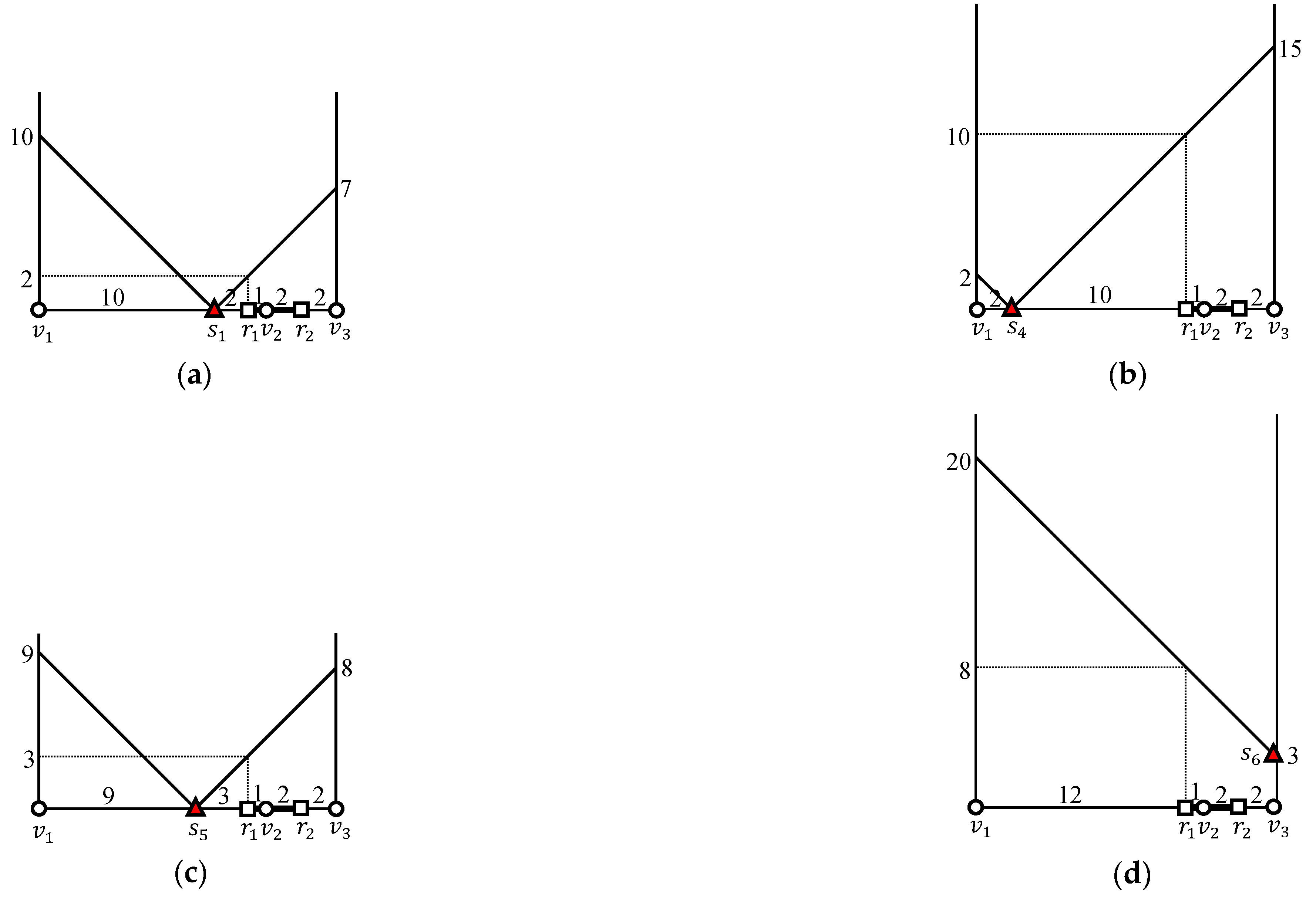
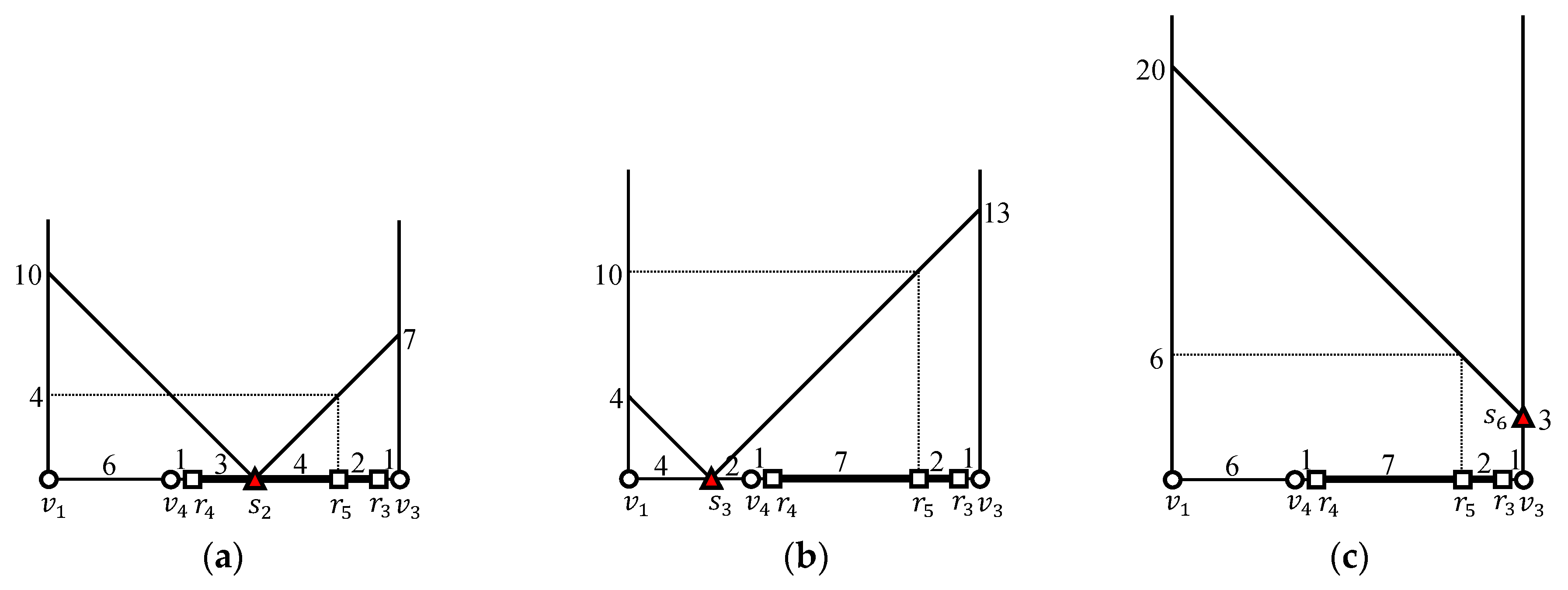
We compute the distance from $r_1$ to each candidate inner object $s\in \left\{s_1,s_4,s_5,s_6\right\}$. Because $s_1\in S\left(\overline{v_1{v}_2{v}_3}\right)-(S_{v_1}^{-2}{\displaystyle \cup }{S}_{v_3}^4)$ according to Table 4, the distance from $r_1$ to $s_1$ is $dist\left(r_1,s_1\right)=len\left(r_1,s_1\right)=2$, as shown in Figure 10a. Because $s_4\in S\left(\overline{v_1{v}_2{v}_3}\right)-\left(S_{v_1}^{-2}{\displaystyle \cup }{S}_{v_3}^4\right)$, the distance from $r_1$ to $s_4$ is $dist\left(r_1,s_4\right)=len\left(r_1,s_4\right)=10$, as shown in Figure 10b. Similarly, because $s_5\in S\left(\overline{v_1{v}_2{v}_3}\right)-\left(S_{v_1}^{-2}{\displaystyle \cup }{S}_{v_3}^4\right)$, the distance from $r_1$ to $s_5$ is $dist\left(r_1,s_5\right)=len\left(r_1,s_5\right)=3$, as shown in Figure 10c. Finally, because $s_6\in S_{v_3}^4-\left(S_{v_1}^{-2}{\displaystyle \cup }S\left(\overline{v_1{v}_2{v}_3}\right)\right)$ according to Table 4, the distance from $r_1$ to $s_6$ is $dist\left(r_1,s_6\right)=len\left(r_1,v_3\right)+dist\left(v_3,s_6\right)=5+3=8$, as shown in Figure 10d. Consequently, $S_{r_1}^{\epsilon }=\left\{s_1,s_5\right\}$ given that $dist\left(r_1,s_1\right)=2$, $dist\left(r_1,s_4\right)=10$, $dist\left(r_1,s_5\right)=3$, and $dist\left(r_1,s_6\right)=8$, and the generated partial join result is $\mathsf{\Phi }\left(r_1\right)=\left\{\left(r_1,s_1\right),\left(r_1,s_5\right)\right\}$.

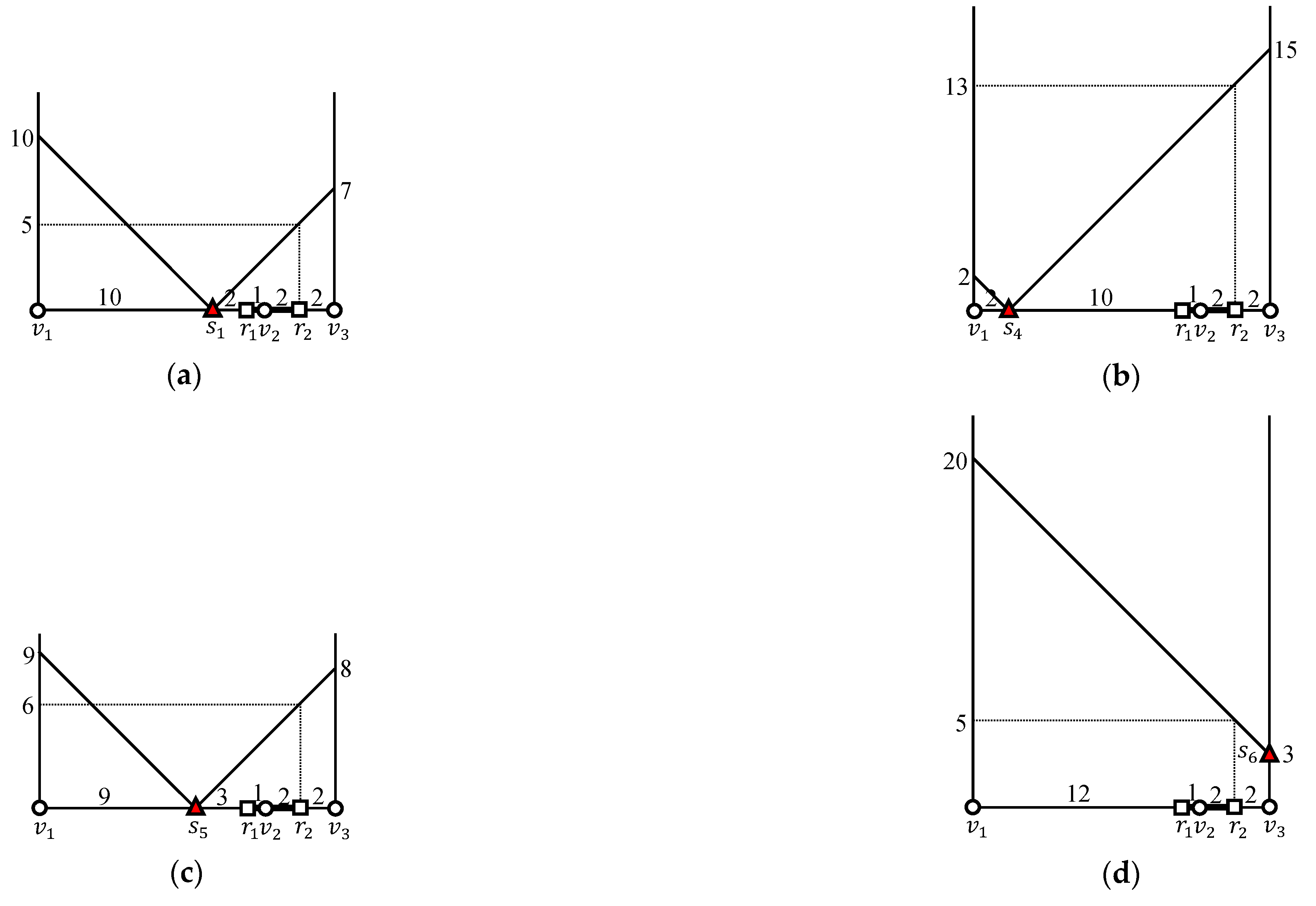
We compute the distance from $r_2$ to each candidate inner object $s\in \left\{s_1,s_4,s_5,s_6\right\}$. Because $s_1\in S\left(\overline{v_1{v}_2{v}_3}\right)-(S_{v_1}^{-2}{\displaystyle \cup }{S}_{v_3}^4)$ according to Table 4, the distance from $r_2$ to $s_1$ is $dist\left(r_2,s_1\right)=len\left(r_2,s_1\right)=5$, as shown in Figure 11a. Because $s_4\in S\left(\overline{v_1{v}_2{v}_3}\right)-(S_{v_1}^{-2}{\displaystyle \cup }{S}_{v_3}^4)$, the distance from $r_2$ to $s_4$ is $dist\left(r_2,s_4\right)=len\left(r_2,s_4\right)=13$, as shown in Figure 11b. In fact, the shortest path from $r_2$ to $s_4$ is $r_2\to v_3\to v_1\to s_4$, whose length is $dist\left(r_2,s_4\right)=9$. However, this deviation from the shortest distance does not affect the query result. Similarly, because $s_5\in S\left(\overline{v_1{v}_2{v}_3}\right)-(S_{v_1}^{-2}{\displaystyle \cup }{S}_{v_3}^4)$, this distance from $r_2$ to $s_5$ is $dist\left(r_2,s_5\right)=len\left(r_2,s_5\right)=6$, as shown in Figure 11c. Finally, because $s_6\in S_{v_3}^4-\left(S_{v_1}^{-2}{\displaystyle \cup }S\left(\overline{v_1{v}_2{v}_3}\right)\right)$ according to Table 4, the distance from $r_2$ to $s_6$ is $dist\left(r_2,s_6\right)=len\left(r_2,v_3\right)+dist\left(v_3,s_6\right)=2+3=5$, as shown in Figure 11d. Consequently, $S_{r_2}^{\epsilon }=\left\{s_1,s_6\right\}$ given that $dist\left(r_2,s_1\right)=5$, $dist\left(r_2,s_4\right)=13$, $dist\left(r_2,s_5\right)=6$, and $dist\left(r_2,s_6\right)=5$, and the generated partial join result is $\mathsf{\Phi }\left(r_2\right)=\left\{\left(r_2,s_1\right),\left(r_2,s_6\right)\right\}$.

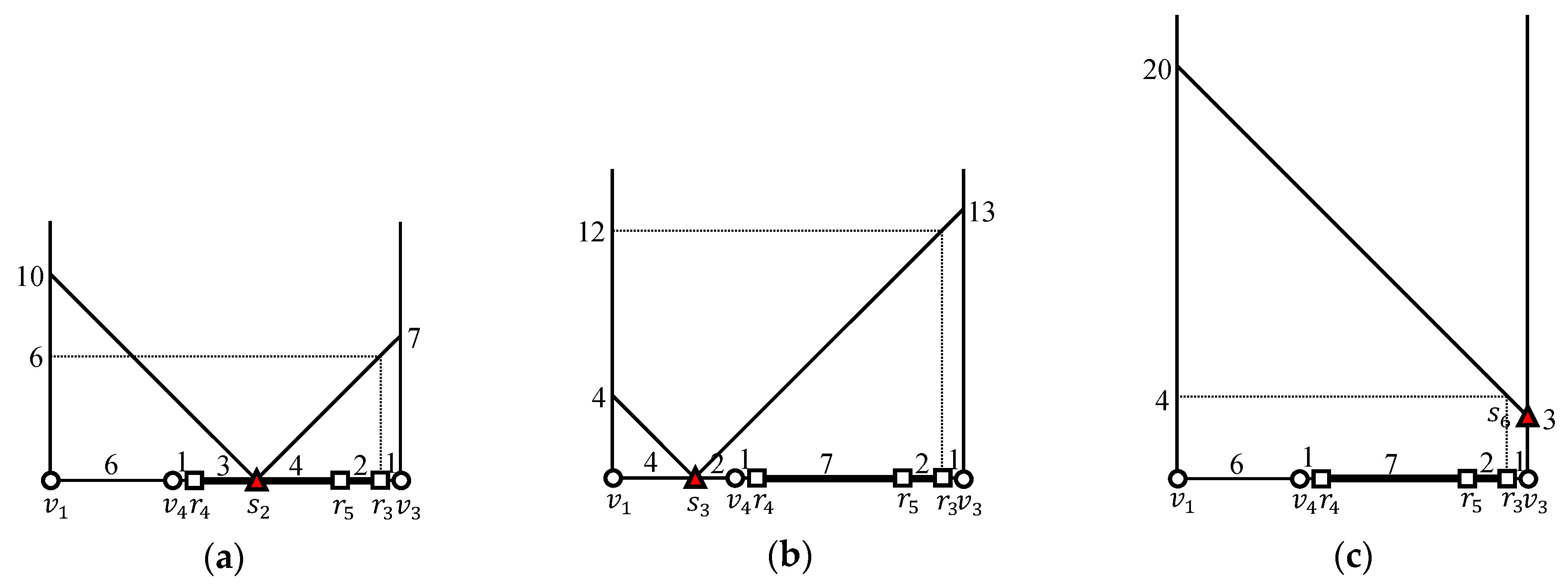
We compute the distance from $r_3$ to each candidate inner object $s\in \left\{s_2,s_3,s_6\right\}$. Because $s_2\in S\left(\overline{v_1{v}_4{v}_3}\right)-\left(S_{v_1}^{-2}{\displaystyle \cup }{S}_{v_3}^4\right)$ according to Table 4, the distance from $r_3$ to $s_2$ is $dist\left(r_3,s_2\right)=len\left(r_3,s_2\right)=6$, as shown in Figure 12a. Similarly, because $s_3\in S\left(\overline{v_1{v}_4{v}_3}\right)-(S_{v_1}^{-2}{\displaystyle \cup }{S}_{v_3}^4)$, the distance from $r_3$ to $s_3$ is $dist\left(r_3,s_3\right)=len\left(r_3,s_3\right)=12$, as shown in Figure 12b. In fact, the shortest path from $r_3$ to $s_3$ is $r_3\to v_3\to v_1\to s_3$, whose length is $dist\left(r_3,s_3\right)=10$. However, this deviation from the shortest distance does not affect the query result. Finally, because $s_6\in S_{v_3}^4-\left(S_{v_1}^{-2}{\displaystyle \cup }\left(\overline{v_1{v}_4{v}_3}\right)\right)$, the distance from $r_3$ to $s_6$ is $dist\left(r_3,s_6\right)=len\left(r_3,v_3\right)+dist\left(v_3,s_6\right)=1+3=4$, as shown in Figure 12c. Consequently, $S_{r_3}^{\epsilon }=\left\{s_6\right\}$ given that $dist\left(r_3,s_2\right)=6$, $dist\left(r_3,s_3\right)=12$, and $dist\left(r_3,s_6\right)=4$, and the generated partial join result is $\mathsf{\Phi }\left(r_3\right)=\left\{\left(r_3,s_6\right)\right\}$.

We compute the distance from $r_4$ to each candidate inner object $s\in \left\{s_2,s_3,s_6\right\}$. Because $s_2\in S\left(\overline{v_1{v}_4{v}_3}\right)-\left(S_{v_1}^{-2}{\displaystyle \cup }{S}_{v_3}^4\right)$ according to Table 4, the distance from $r_4$ to $s_2$ is $dist\left(r_4,s_2\right)=len\left(r_4,s_2\right)=3$, as shown in Figure 13a. Similarly, because $s_3\in S\left(\overline{v_1{v}_4{v}_3}\right)-\left(S_{v_1}^{-2}{\displaystyle \cup }{S}_{v_3}^4\right)$, the distance from $r_4$ to $s_3$ is $dist\left(r_4,s_3\right)=len\left(r_4,s_3\right)=3$, as shown in Figure 13b. Finally, because $s_6\in S_{v_3}^4-\left(S_{v_1}^{-2}{\displaystyle \cup }S\left(\overline{v_1{v}_4{v}_3}\right)\right)$, the distance from $r_4$ to $s_6$ is $dist\left(r_4,s_6\right)=len\left(r_4,v_3\right)+dist\left(v_3,s_6\right)=10+3=13$, as shown in Figure 13c. In fact, the shortest path from $r_4$ to $s_6$ is $r_4\to v_4\to v_1\to s_6$, whose length is $dist\left(r_4,s_6\right)=9$. However, this deviation from the shortest distance does not affect the query result. Consequently, $S_{r_4}^{\epsilon }=\left\{s_2,s_3\right\}$ given that $dist\left(r_4,s_2\right)=3$, $dist\left(r_4,s_3\right)=3$, and $dist\left(r_4,s_6\right)=13$, and the generated partial join result is $\mathsf{\Phi }\left(r_4\right)=\left\{\left(r_4,s_2\right),\left(r_4,s_3\right)\right\}$.

We compute the distance from $r_5$ to each candidate inner object $s\in \left\{s_2,s_3,s_6\right\}$. Because $s_2\in S\left(\overline{v_1{v}_4{v}_3}\right)-\left(S_{v_1}^{-2}{\displaystyle \cup }{S}_{v_3}^4\right)$ according to Table 4, the distance from $r_5$ to $s_2$ is $dist\left(r_5,s_2\right)=len\left(r_5,s_2\right)=4$, as shown in Figure 14a. Similarly, because $s_3\in S\left(\overline{v_1{v}_4{v}_3}\right)-\left(S_{v_1}^{-2}{\displaystyle \cup }{S}_{v_3}^4\right)$, the distance from $r_5$ to $s_3$ is $dist\left(r_5,s_3\right)=len\left(r_5,s_3\right)=10$, as shown in Figure 14b. Finally, because $s_6\in S_{v_3}^4-\left(S_{v_1}^{-2}{\displaystyle \cup }S\left(\overline{v_1{v}_4{v}_3}\right)\right)$, the distance from $r_5$ to $s_6$ is $dist\left(r_5,s_6\right)=len\left(r_5,v_3\right)+dist\left(v_3,s_6\right)=3+3=6$, as shown in Figure 14c. Consequently, $S_{r_5}^{\epsilon }=\left\{s_2\right\}$ given that $dist\left(r_5,s_2\right)=4$, $dist\left(r_5,s_3\right)=10$, and $dist\left(r_5,s_6\right)=6$, and the generated partial join result is $\mathsf{\Phi }\left(r_5\right)=\left\{\left(r_5,s_2\right)\right\}$. Finally, we obtain the complete query result $\mathsf{\Phi }\left(R\right)=\mathsf{\Phi }\left(r_1\right){\displaystyle \cup }\mathsf{\Phi }\left(r_2\right){\displaystyle \cup }\mathsf{\Phi }\left(r_3\right){\displaystyle \cup }\mathsf{\Phi }\left(r_4\right){\displaystyle \cup }\mathsf{\Phi }\left(r_5\right)=\left\{\left(r_1,s_1\right),\left(r_1,s_5\right),\left(r_2,s_1\right),\left(r_2,s_6\right),\left(r_3,s_6\right),\left(r_4,s_2\right),\left(r_4,s_3\right),\left(r_5,s_2\right)\right\}$.

6. Performance Study

In this section, we report on an empirical analysis of our proposed solution. We present our experimental settings in Section 6.1, followed by our experimental results in Section 6.2.

6.1. Experimental Settings

For the performance study, we use three real-world road networks [43], which are described in

Table 5. Real-world roadmaps.

Name	Description	Number of Vertices	Number of Edges	Number of Vertex Sequences
CAL	California and Nevada	1,890,815	2,315,222	1,794,708
FLA	Florida	1,070,376	1,343,951	1,100,675
COL	Colorado	435,666	521,200	374,355

. These real-world road networks have different sizes and are part of the US’s road network.

Table 6. Experimental parameter settings.

Parameter	Range
Threshold distance ($\epsilon$)	0.005, 0.01, 0.03, 0.05, 0.1
Numbers of outer objects ($\left|R\right|$) and inner objects ($\left|S\right|$)	1, 5, 10, 20, 30 ($\times {10}^3$) for CAL and FLA 1, 3, 5, 7, 10 ($\times {10}^3$) for COL
Distributions of outer objects	(C)entroid, (U)niform
Distributions of inner objects	(C)entroid, (U)niform
Real-world roadmaps	CAL, FLA, COL

shows the range of each variable used in the experiments with defaults indicated in bold. For convenience, each dimension of the data universe is normalized independently to unit length, such that the threshold distance $\epsilon$ is in the range of $\left[0,1\right]$. The positions of both the outer objects and the inner objects follow either centroid or uniform distributions. The centroid dataset is generated to resemble the real-world data. First, 10 centroids are selected randomly. The objects around each centroid follow a normal distribution, where the mean is set to the centroid and the standard deviation is set to 1% of the side length of the data universe. In each experiment, we vary one or two of the parameters within the range shown in Table 6, while keeping other parameters at default values. The outer objects and the inner objects follow the centroid distribution unless stated otherwise.

We implement and evaluate two versions of our proposed solution, i.e., the naive EDISON and EDISON methods. As a benchmark for our proposed method, we use a baseline method that computes the range query of every outer object using the RNE algorithm [10]. A comparison with the pre-computed distance-based solution [23] and the Euclidean distance-based solution (e.g., JER [10]) is beyond the scope of this study, because these methods cannot support frequent network traffic updates.

All algorithms are implemented in C++ in Microsoft Visual Studio 2015, and they use common subroutines for similar tasks. We conduct experiments on a desktop computer running Windows 10 with a 4 GHz processor and 32 GB of memory. We believe that indexing structures of all techniques should be memory resident to ensure responsive query processing, which is assumed in many recent studies [5,11] and is crucial to online map services and commercial navigation systems. We determine the average values based on 10 repetitions of the experiments for each algorithm.

6.2. Experimental Results

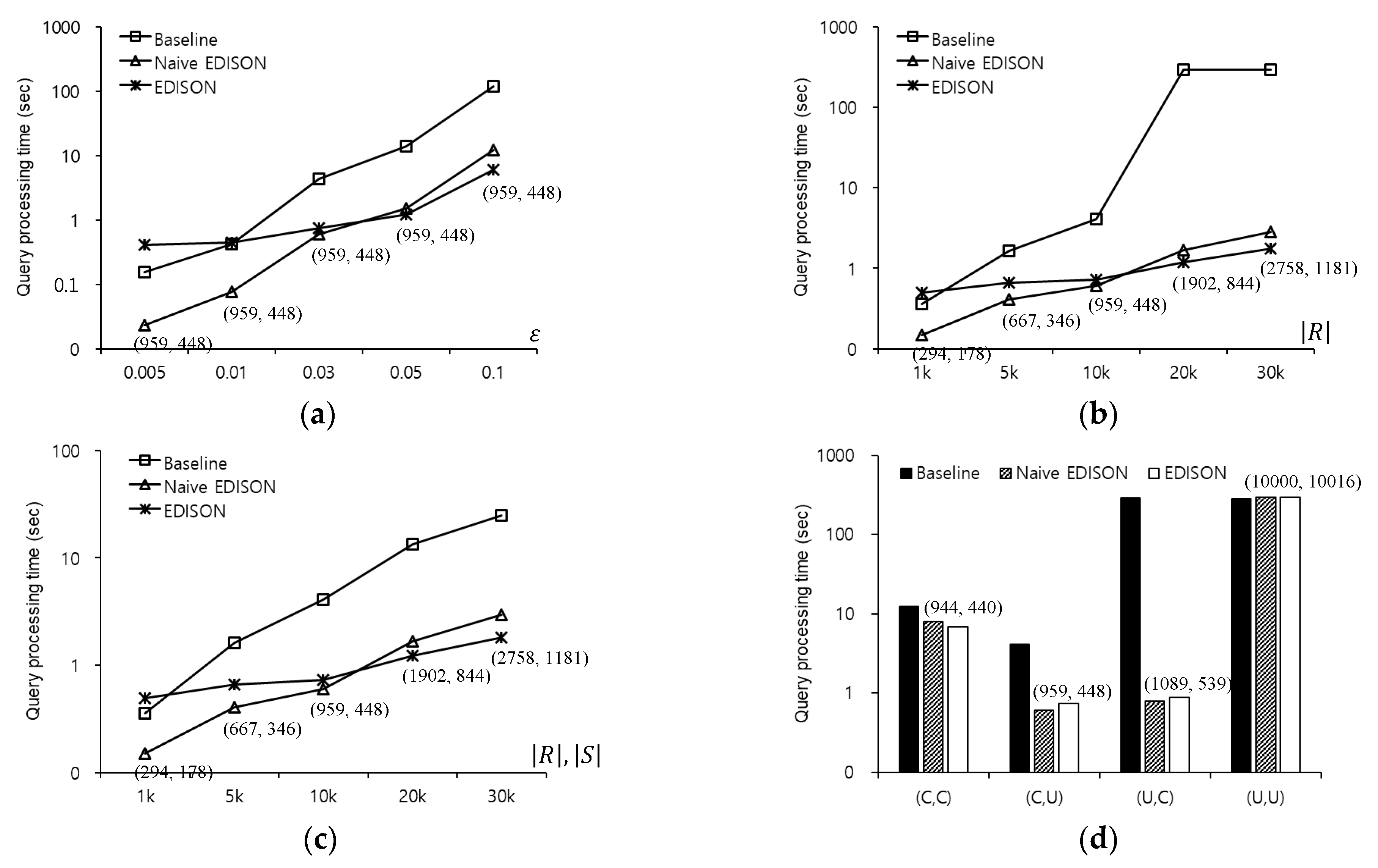
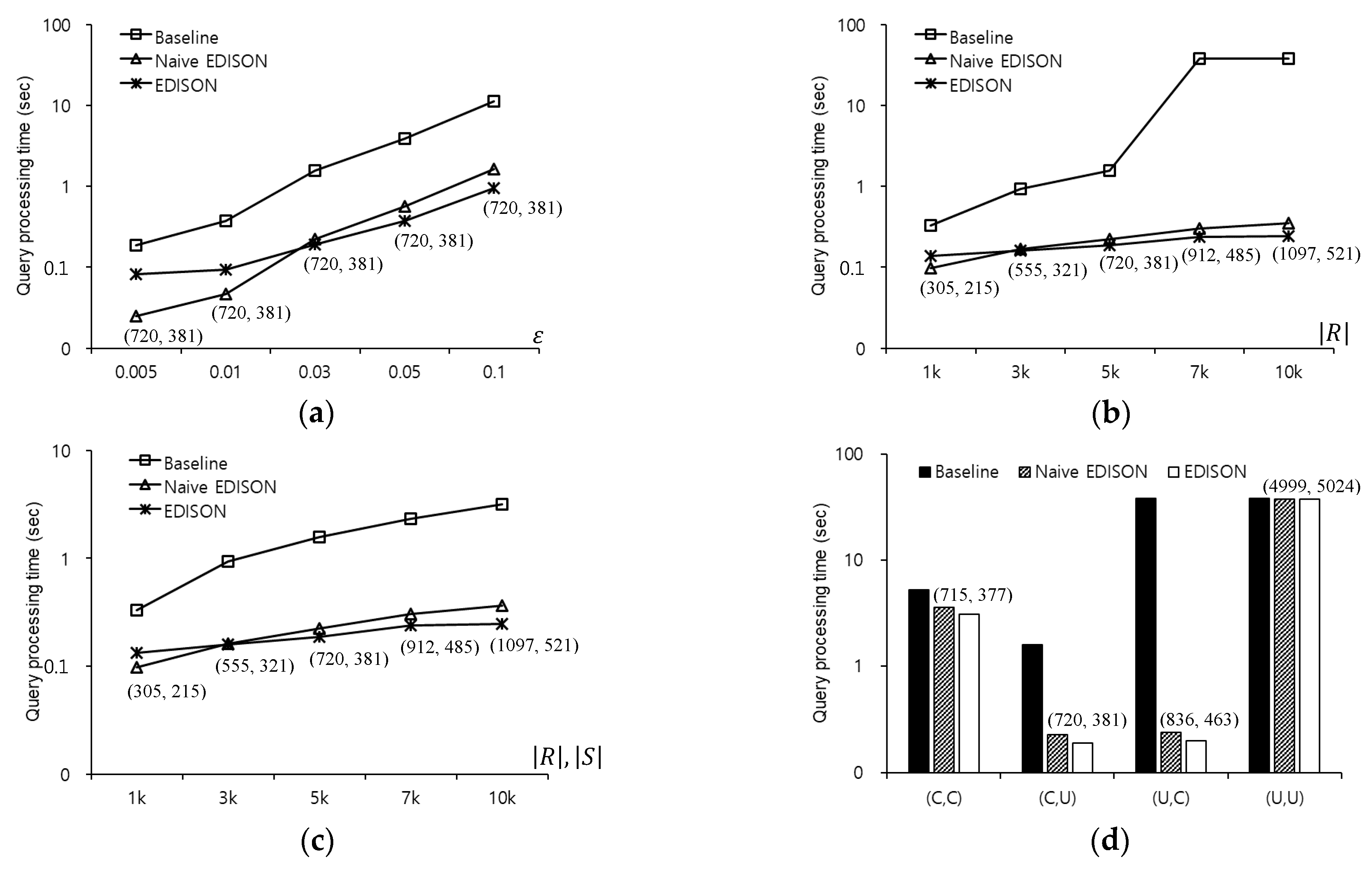
Figure 15 compares the query processing times using the baseline, naive EDISON, and EDISON methods to evaluate $\epsilon$-distance join queries in the CAL roadmap, where each chart illustrates the effect of changing one or two of the parameters in Table 6. The first and the second values in parentheses indicate the number of range queries that are evaluated by the naive EDISON and EDISON methods, respectively. The numbers of range queries evaluated by the baseline method are omitted, because these numbers become $min\left\{\left|R\right|,\left|S\right|\right\}$, i.e., the cardinality of the smaller dataset between $\left|R\right|$ and $\left|S\right|$. Figure 15a shows the query processing time as a function of the threshold distance $\epsilon$. Although the EDISON method shows the worst performance for $\epsilon =0.005$, the processing times using the baseline and the naive EDISON methods increase more rapidly with the value of $\epsilon$ than those using the EDISON method. This implies that the shared execution of the EDISON method is more effective for a large threshold distance $\epsilon$. The baseline, naive EDISON, and EDISON methods evaluate a total of 10,000 range queries, 959 range queries, and 448 range queries, respectively. Figure 15b shows the query processing time as a function of the number $\left|R\right|$ of outer objects, while the number of inner objects is fixed at $\left|S\right|=10,000$. The EDISON method is less sensitive to variations in $\left|R\right|$ than the other methods, although it shows the worst performance at $\left|R\right|=1000$. Owing to the benefit of the shared execution processing, the numbers of range queries evaluated by the naive EDISON and EDISON methods increase slightly with $\left|R\right|$.

Figure 15c shows the query processing time as a function of both the number $\left|R\right|$ of outer objects and the number $\left|S\right|$ of inner objects. The naive EDISON method outperforms the EDISON method for $1000\le \left|R\right|,\left|\mathrm{S}\right|\le 10,000,$ whereas the latter outperforms the former for $20,000\le \left|R\right|,\left|\mathrm{S}\right|\le 30,000$. This indicates that the EDISON method optimizes the shared execution processing more effectively than the naive EDISON method for large datasets. Clearly, the baseline method shows the worst performance in most cases. Figure 15d shows the query processing time for various distributions of outer objects and inner objects, where each ordered pair (i.e., $\left(\mathrm{C},\mathrm{C}\right)$, $\left(\mathrm{C},\mathrm{U}\right)$, $\left(\mathrm{U},\mathrm{C}\right)$, and $\left(\mathrm{U},\mathrm{U}\right)$) denotes a combination of the distributions of outer objects and inner objects. Because shared execution processing is favorable for non-uniform distributions of objects, the naive EDISON and EDISON methods significantly outperform the baseline method for $\left(\mathrm{C},\mathrm{C}\right)$, $\left(\mathrm{C},\mathrm{U}\right)$, and $\left(\mathrm{U},\mathrm{C}\right)$. However, the processing times of the naive EDISON and EDISON methods for $\left(\mathrm{U},\mathrm{U}\right)$ are very similar to the baseline method. This is because both the outer objects and the inner objects are widely scattered, which hinders shared execution processing.

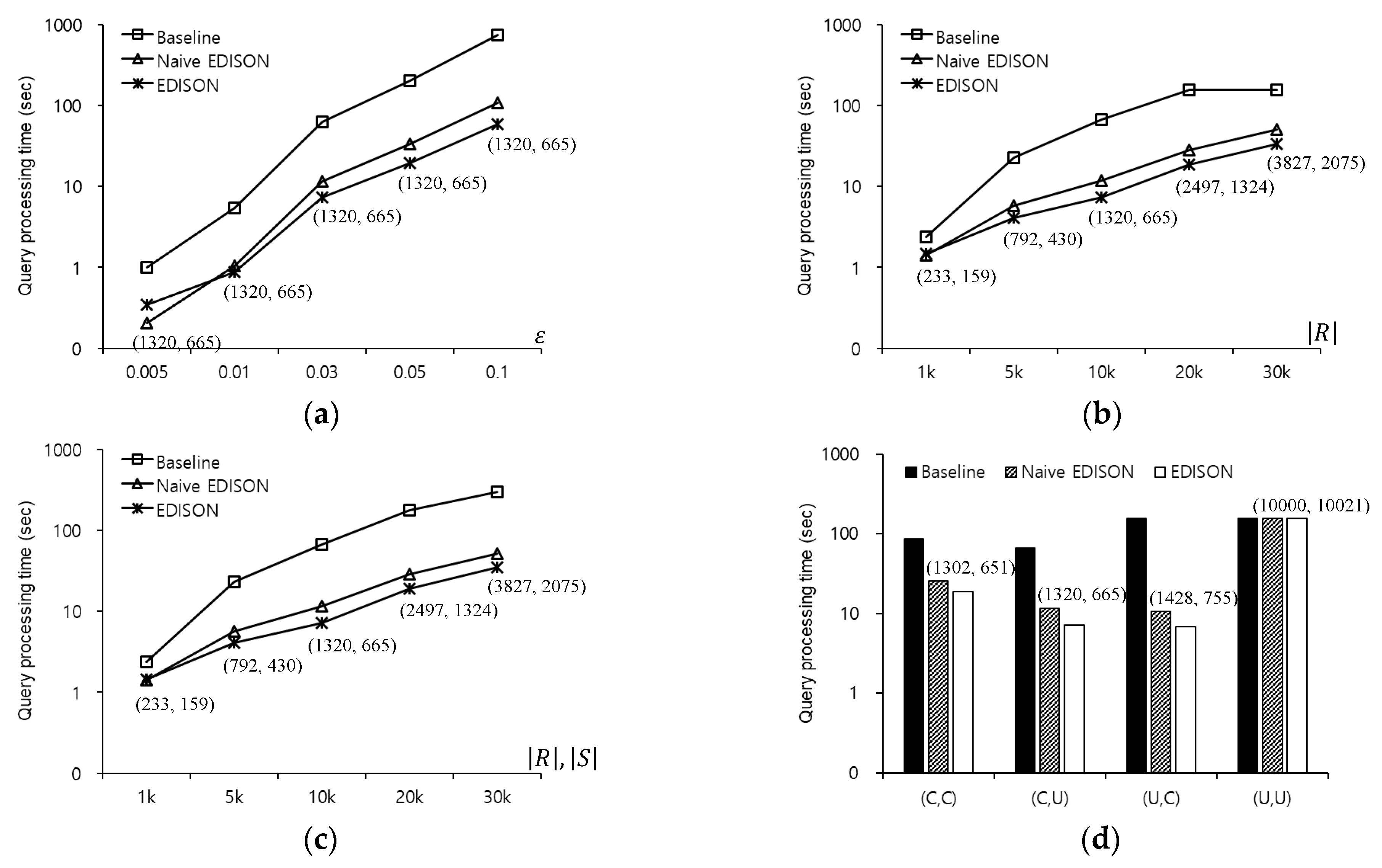
Figure 16 compares the query processing times using the baseline, naive EDISON, and EDISON methods to evaluate $\epsilon$-distance join queries in the FLA roadmap. Figure 16a shows the query processing time as a function of $\epsilon$, when $\epsilon$ varies between 0.005 and 0.1. The EDISON method achieves the best performance for $0.01\le \epsilon \le 0.1$, because it evaluates the smallest number of range queries among the three methods. The baseline, naive EDISON, and EDISON methods evaluate 10,000 range queries, 1320 range queries, and 665 range queries, respectively. Figure 16b shows the query processing time as a function of $\left|R\right|$, when $\left|R\right|$ varies between 1000 and 30,000. The EDISON method clearly outperforms the other methods for $5000\le \left|R\right|\le 30,000$. Due to shared execution processing, the naive EDISON and EDISON methods are less sensitive to changes in $\left|R\right|$ than the baseline method. Figure 16c shows the query processing time as a function of $\left|R\right|$ and $\left|S\right|$, when $\left|R\right|$ ($\left|S\right|$) varies between 1000 and 30,000. The EDISON method clearly outperforms the other methods for $5000\le \left|R\right|,\left|S\right|\le 30,000$. Figure 16d shows the query processing time for various distributions of outer objects and inner objects. The naive EDISON and EDISON methods significantly outperform the baseline method for $\left(\mathrm{C},\mathrm{C}\right)$, $\left(\mathrm{C},\mathrm{U}\right)$, and $\left(\mathrm{U},\mathrm{C}\right)$, whereas the former methods show similar performance to the latter method for $\left(\mathrm{U},\mathrm{U}\right)$ for the same reason as in the CAL case.

Figure 17 compares the query processing times using the baseline, naive EDISON, and EDISON methods to evaluate $\epsilon$-distance join queries in the COL roadmap. Figure 17a shows the query processing time as a function of $\epsilon$, when $\epsilon$ varies between 0.005 and 0.1. The naive EDISON and EDISON methods significantly outperform the baseline method in all cases. Specifically, the query processing time of the EDISON method is up to 11 times shorter than the baseline method at $\epsilon =0.1$. The naive EDISON method significantly outperforms the EDISON method for $0.005\le \epsilon \le 0.01$, whereas the latter outperforms the former for $0.03\le \epsilon \le 0.1$. This indicates that the EDISON method is less sensitive to changes in $\epsilon$ than the naive EDISON method. Figure 17b shows the query processing time as a function of $\left|R\right|$, when $\left|R\right|$ varies between 1000 and 10,000. The naive EDISON and EDISON methods significantly outperform the baseline method in all cases and the former methods are less sensitive to changes in $\left|R\right|$ than the latter method. This indicates that the performance difference between the EDISON method and the baseline method increases rapidly with $\left|R\right|$. Specifically, the query processing time of the EDISON method is up to 155 times shorter than the baseline method at $\left|R\right|=10,000$. Figure 17c shows the query processing time as a function of $\left|R\right|$ and $\left|S\right|$, when $\left|R\right|$ ($\left|S\right|$) varies between 1000 and 10,000. The naive EDISON method outperforms the EDISON method at $\left|R\right|=\left|S\right|=1000$, whereas the latter outperforms the former for $5000\le \left|R\right|,\left|S\right|\le 10,000,$ and the performance difference between the two methods increases with $\left|R\right|$. and $\left|S\right|$. This implies that the EDISON method scales better with $\left|R\right|$ and $\left|S\right|$ than the naive EDISON method. Figure 17d shows the query processing time for various distributions of outer objects and inner objects. The naive EDISON and EDISON methods significantly outperform the baseline method for $\left(\mathrm{C},\mathrm{C}\right)$, $\left(\mathrm{C},\mathrm{U}\right)$, and $\left(\mathrm{U},\mathrm{C}\right)$. However, all methods show similar performance when the outer objects and the inner objects follow uniform distributions $\left(\mathrm{U},\mathrm{U}\right)$. This is expected because both the outer objects and inner objects are widely scattered for $\left(\mathrm{U},\mathrm{U}\right)$, which obstructs shared execution processing of the naive EDISON and EDISON methods.

7. Conclusions

In this study, we investigated the efficient processing of $\epsilon$-distance join queries in dynamic road networks. We proposed a cost-effective solution called EDISON that optimizes the shared execution method to avoid redundant network traversal. We implemented and evaluated a baseline method and two versions of EDISON, i.e., the naive EDISON and EDISON methods. The experiments are based on several real-world roadmaps and involve a wide range of parameter values. The experimental results are summarized as follows: (1) the naive EDISON and EDISON methods significantly outperform the baseline method; (2) the naive EDISON and EDISON methods are typically comparable in terms of query processing time; (3) the EDISON method scales better with increasing number of objects and threshold distance than the naive EDISON method. In future work, we plan to extend the shared execution approach used here to the problems of processing sophisticated spatial queries over road networks, such as multi-way distance join queries [44] and aggregate k-farthest neighbor queries [45,46]. These problems have not been adequately addressed with regard to road networks despite their importance.

References

- Delling, D.; Goldberg, A.V.; Pajor, T.; Werneck, R.F. Customizable route planning in road networks. Transp. Sci. 2017, 51, 566–591. [Google Scholar] [CrossRef]
- Samet, H.; Sankaranarayanan, J.; Alborzi, H. Scalable network distance browsing in spatial databases. In Proceedings of the International Conference on Management of Data, Vancouver, BC, Canada, 10–12 June 2008. [Google Scholar]
- Sankaranarayanan, J.; Alborzi, H.; Samet, H. Efficient query processing on spatial networks. In Proceedings of the International Workshop on Geographic Information Systems, Bremen, Germany, 4–5 November 2005. [Google Scholar]
- Sankaranarayanan, J.; Samet, H.; Alborzi, H. Path oracles for spatial networks. PVLDB 2009, 2, 1210–1221. [Google Scholar] [CrossRef] [Green Version]
- Wu, L.; Xiao, X.; Deng, D.; Cong, G.; Zhu, A.D.; Zhou, S. Shortest path and distance queries on road networks: An experimental evaluation. PVLDB 2012, 5, 406–417. [Google Scholar] [CrossRef]
- Zhang, D.; Yang, D.; Wang, Y.; Tan, K.-L.; Cao, J.; Shen, H.T. Distributed shortest path query processing on dynamic road networks. VLDB J. 2017, 26, 399–419. [Google Scholar] [CrossRef]
- Zhong, R.; Li, G.; Tan, K.-L.; Zhou, L.; Gong, Z. G-tree: An efficient and scalable index for spatial search on road networks. IEEE Trans. Knowl. Data Eng. 2015, 27, 2175–2189. [Google Scholar] [CrossRef]
- D’Angelo, G.; D’Emidio, M.; Frigioni, D. Distance queries in large-scale fully dynamic complex networks. In Proceedings of the International Workshop on Combinatorial Algorithms, Helsinki, Finland, 17–19 August 2016. [Google Scholar]
- Sankaranarayanan, J.; Samet, H. Query processing using distance oracles for spatial networks. IEEE Trans. Knowl. Data Eng. 2010, 22, 1158–1175. [Google Scholar] [CrossRef]
- Papadias, D.; Zhang, J.; Mamoulis, N.; Tao, Y. Query processing in road network databases. In Proceedings of the International Conference on Very Large Data Bases, Berlin, Germany, 9–12 September 2003. [Google Scholar]
- Abeywickrama, T.; Cheema, M.A.; Taniar, D. k-Nearest neighbors on road networks: A journey in experimentation and in-memory implementation. PVLDB 2016, 9, 492–503. [Google Scholar] [CrossRef]
- Luo, S.; Kao, B.; Li, G.; Hu, J.; Cheng, R.; Zheng, Y. TOAIN: A throughput optimizing adaptive index for answering dynamic knn queries on road networks. PVLDB 2018, 11, 594–606. [Google Scholar]
- Chaudhuri, S.; Ganti, V.; Kaushik, R. A primitive operator for similarity joins in data cleaning. In Proceedings of the International Conference on Data Engineering, Atlanta, GA, USA, 3–8 April 2006. [Google Scholar]
- Deng, D.; Li, G.; Hao, S.; Wang, J.; Feng, J. MassJoin: A mapreduce-based method for scalable string similarity joins. In Proceedings of the International Conference on Data Engineering, Chicago, IL, USA, 31 March–4 April 2014. [Google Scholar]
- Metwally, A.; Faloutsos, C. V-SMART-Join: A scalable mapreduce framework for all-pair similarity joins of multisets and vectors. PVLDB 2012, 5, 704–715. [Google Scholar] [CrossRef]
- Sarma, A.D.; He, Y.; Chaudhuri, S. ClusterJoin: A similarity joins framework using map-reduce. PVLDB 2014, 7, 1059–1070. [Google Scholar]
- Vernica, R.; Carey, M.J.; Li, C. Efficient parallel set-similarity joins using mapreduce. In Proceedings of the International Conference on Management of Data, Indianapolis, IN, USA, 6–10 June 2010. [Google Scholar]
- Wang, Y.; Metwally, A.; Parthasarathy, S. Scalable all-pairs similarity search in metric spaces. In Proceedings of the International Conference on Knowledge Discovery and Data Mining, Chicago, IL, USA, 11–14 August 2013. [Google Scholar]
- Hjaltason, G.R.; Samet, H. Incremental distance join algorithms for spatial databases. In Proceedings of the International Conference on Management of Data, Seattle, WA, USA, 2–4 June 1998. [Google Scholar]
- Shin, H.; Moon, B.; Lee, S. Adaptive and incremental processing for distance join queries. IEEE Trans. Knowl. Data Eng. 2003, 15, 1561–1578. [Google Scholar] [CrossRef]
- Mahmud, H.; Amin, A.M.; Ali, M.E.; Hashem, T.; Nutanong, S. A group based approach for path queries in road networks. In Proceedings of the International Symposium on Spatial and Temporal Databases, Munich, Germany, 21–23 August 2013. [Google Scholar]
- Mouratidis, K.; Yiu, M.L.; Papadias, D.; Mamoulis, N. Continuous nearest neighbor monitoring in road networks. In Proceedings of the International Conference on Very Large Data Bases, Seoul, Korea, 12–15 September 2006. [Google Scholar]
- Sankaranarayanan, J.; Alborzi, H.; Samet, H. Distance join queries on spatial networks. In Proceedings of the International Symposium on Geographic Information Systems, Arlington, VA, USA, 10–11 November 2006. [Google Scholar]
- Arain, Q.A.; Deng, Z.; Memon, I.; Zubedi, A.; Jiao, J.; Ashraf, A.; Khan, M.S. Privacy protection with dynamic pseudonym-based multiple mix-zones over road networks. China Commun. 2017, 14, 89–100. [Google Scholar] [CrossRef]
- Arain, Q.A.; Memon, I.; Deng, Z.; Memon, M.H.; Mangi, F.A.; Zubedi, A. Location monitoring approach: Multiple mix-zones with location privacy protection based on traffic flow over road networks. Multimedia Tools Appl. 2018, 77, 5563–5607. [Google Scholar] [CrossRef]
- Arain, Q.A.; Uqaili, M.A.; Deng, Z.; Memon, I.; Jiao, J.; Shaikh, M.A.; Zubedi, A.; Ashraf, A.; Arain, U.A. Clustering based energy efficient and communication protocol for multiple mix-zones over road networks. Wirel. Pers. Commun. 2017, 95, 411–428. [Google Scholar] [CrossRef]
- Domenic, M.K.; Wang, Y.; Zhang, F.; Memon, I.; Gustav, Y.H. Preserving users’ privacy for continuous query services in road networks. In Proceedings of the International Conference on Information Management, Innovation Management and Industrial Engineering, Xi’an, China, 23–24 November 2013. [Google Scholar]
- Gustav, Y.H.; Wang, Y.; Domenic, M.K.; Zhang, F.; Memon, I. Velocity similarity anonymization for continuous query Location based services. In Proceedings of the International Conference on Computational Problem-Solving, Jiuzhai, China, 26–28 October 2013. [Google Scholar]
- Kamenyi, D.M.; Wang, Y.; Zhang, F.; Memon, I. Authenticated privacy preserving for continuous query in location based services. J. Comput. Inform. Syst. 2013, 9, 9857–9864. [Google Scholar]
- Memon, I. Distance and clustering-based energy-efficient pseudonyms changing strategy over road network. Int. J. Commun. Syst. 2018, 31, 1–22. [Google Scholar] [CrossRef]
- Memon, I. Authentication user’s privacy: An integrating location privacy protection algorithm for secure moving objects in location based services. Wirel. Pers. Commun. 2015, 82, 1585–1600. [Google Scholar] [CrossRef]
- Memon, I.; Arain, Q.A. Dynamic path privacy protection framework for continuous query service over road networks. World Wide Web 2017, 20, 639–672. [Google Scholar] [CrossRef]
- Memon, I.; Arain, Q.A.; Zubedi, A.; Mangi, F.A. DPMM: Dynamic pseudonym-based multiple mix-zones generation for mobile traveler. Multimedia Tools Appl. 2017, 76, 24359–24388. [Google Scholar] [CrossRef]
- Memon, I.; Chen, L.; Arain, Q.A.; Memon, H.; Chen, G. Pseudonym changing strategy with multiple mix zones for trajectory privacy protection in road networks. Int. J. Commun. Syst. 2018, 31, 1–44. [Google Scholar] [CrossRef]
- Ali, M.E.; Tanin, E.; Zhang, R.; Kulik, L. A motion-aware approach for efficient evaluation of continuous queries on 3D object databases. VLDB J. 2010, 19, 603–632. [Google Scholar] [CrossRef]
- Giannikis, G.; Alonso, G.; Kossmann, D. SharedDB: Killing one thousand queries with one stone. PVLDB 2012, 5, 526–537. [Google Scholar] [CrossRef]
- Thomsen, J.R.; Yiu, M.L.; Jensen, C.S. Effective caching of shortest paths for location-based services. In Proceedings of the International Conference on Management of Data, Scottsdale, AZ, USA, 20–24 May 2012. [Google Scholar]
- Zhang, D.; Chow, C.-Y.; Li, Q.; Zhang, X.; Xu, Y. SMashQ: Spatial mashup framework for k-nn queries in time-dependent road networks. Distrib. Parall. Databases 2013, 31, 259–287. [Google Scholar] [CrossRef]
- Brinkhoff, T.; Kriegel, H.-P.; Seeger, B. Efficient processing of spatial joins using r-trees. In Proceedings of the International Conference on Management of Data, Washington, DC, USA, 26–28 May 1993. [Google Scholar]
- Chen, C.; Sun, W.; Zheng, B.; Mao, D.; Liu, W. An incremental approach to closest pair queries in spatial networks using best-first search. In Proceedings of the International Conference on Database and Expert Systems Applications, Toulouse, France, 29 August–2 September 2011. [Google Scholar]
- Koudas, N.; Sevcik, K.C. High dimensional similarity joins: Algorithms and performance evaluation. IEEE Trans. Knowl. Data Eng. 2000, 12, 3–18. [Google Scholar] [CrossRef]
- Makreshanski, D.; Giannikis, G.; Alonso, G.; Kossmann, D. MQJoin: Efficient shared execution of main-memory joins. PVLDB 2016, 9, 480–491. [Google Scholar] [CrossRef]
- 9th DIMACS Implementation Challenge: Shortest Paths. Available online: http://www.dis.uniroma1.it/challenge9/download.shtml (accessed on 15 June 2018).
- Corral, A.; Manolopoulos, Y.; Theodoridis, Y.; Vassilakopoulos, M. Multi-way distance join queries in spatial databases. GeoInformatica 2004, 8, 373–402. [Google Scholar] [CrossRef]
- Gao, Y.; Shou, L.; Chen, K.; Chen, G. Aggregate farthest-neighbor queries over spatial data. In Proceedings of the International Conference on Database Systems for Advanced Applications, Hong Kong, China, 22–25 April 2011. [Google Scholar]
- Wang, H.; Zheng, K.; Su, H.; Wang, J.; Sadiq, S.; Zhou, X. Efficient aggregate farthest neighbour query processing on road networks. In Proceedings of the Australasian Database Conference, Brisbane, Australia, 14–16 July 2014. [Google Scholar]
Figure 1.
Example of dynamic road networks (a) traffic condition at time ; (b) traffic condition at time .
Figure 2.
Example where and .
Figure 3.
Example of an -distance join query in a road network.
Figure 4.
Grouping outer and inner objects (a) and ; (b) and .
Figure 5.
Determination of the distance from to (a) If , then ; (b) If , then ; (c) If , then .
Figure 6.
Computation of the distance from to (a) If , ; (b) If , .
Figure 7.
Computation of the distance from to (a) ; (b) ; (c) .
Figure 8.
Investigating the number of outer segments adjacent to an intersection vertex (a) ; (b) ; (c) .
Figure 9.
Simple heuristic .
Figure 10.
Computation of the distance from to (a) ; (b) ; (c) ; (d) .
Figure 11.
Figure 12.
Figure 13.
Figure 14.
Figure 15.
Comparison of the baseline, naive EDISON, and EDISON methods for CAL (a) varying ; (b) varying ; (c) varying and ; (d) varying the distributions of objects.
Figure 16.
Comparison of the baseline, naive EDISON, and EDISON methods for FLA (a) varying ; (b) varying ; (c) varying and ; (d) varying the distributions of objects.
Figure 17.
Comparison of the baseline, naive EDISON, and EDISON methods for COL (a) varying ; (b) varying ; (c) varying and ; (d) varying the distributions of objects.