Article

Semi-Automatic Versus Manual Mapping of Cold-Water Coral Carbonate Mounds Located Offshore Norway

Norges geologiske undersøkelse (Geological Survey of Norway), Postboks 6315 Torgarden, 7491 Trondheim, Norway
*
Author to whom correspondence should be addressed.
ISPRS Int. J. Geo-Inf. 2019, 8(1), 40; https://doi.org/10.3390/ijgi8010040
Submission received: 2 November 2018 / Revised: 21 December 2018 / Accepted: 10 January 2019 / Published: 16 January 2019
(This article belongs to the Special Issue GEOBIA in a Changing World)

Abstract

:
Cold-water coral reefs are hotspots of biological diversity and play an important role as carbonate factories in the global carbon cycle. Reef-building corals can be found in cold oceanic waters around the world. Detailed knowledge on the spatial location and distribution of coral reefs is of importance for spatial management, conservation and science. Carbonate mounds (reefs) are readily identifiable in high-resolution multibeam echosounder data but systematic mapping programs have relied mostly on visual interpretation and manual digitizing so far. Developing more automated methods will help to reduce the time spent on this laborious task and will additionally lead to more objective and reproducible results. In this paper, we present an attempt at testing whether rule-based classification can replace manual mapping when mapping cold-water coral carbonate mounds. To that end, we have estimated and compared the accuracies of manual mapping, pixel-based terrain analysis and object-based image analysis. To verify the mapping results, we created a reference dataset of presence/absence points agreed upon by three mapping experts. There were no statistically significant differences in the overall accuracies of the maps produced by the three approaches. We conclude that semi-automated rule-based methods might be a viable option for mapping carbonate mounds with high spatial detail over large areas.

1. Introduction

Coral reefs, which are frequently associated with warm, shallow and photic tropical seas, are also found widespread in deep waters of continental shelves, slopes, seamounts and ridge systems around the world [1]. Such cold-water coral (CWC) reefs are of high importance since they contribute to increased biodiversity [2], create suitable conditions for nurseries for fish larvae [3,4], provide food to many organisms [5,6] and act as carbonate factories [7,8].
At the same time, CWC reefs are fragile and slow-growing three-dimensional structures that are vulnerable to various anthropogenic impacts, such as demersal fishing [9,10,11], mining [12], hydrocarbon drilling [13] and climate change (ocean warming [14] and acidification [6,15]). Knowledge about their spatial distribution and habitat requirements is crucial to be able to prevent or minimize damage to CWC reefs.
CWCs are generally restricted to oceanic waters with temperatures of 4–12 °C, which translates to water depths of approximately 50–1000 m at high latitudes and down to 4000 m at low latitudes [1]. CWCs in the north-east Atlantic Ocean tolerate a wide range of environmental conditions although they appear to be limited to intermediate water masses within a certain density envelope [16]. At local scales, CWC occurrence is linked to the availability of fresh labile organic matter [17] and the presence of hard substrate for larval settlement. CWC reefs frequently occur on positive-relief landforms, such as bedrock ridges and submarine slide terrains [18,19]. Glacial landforms, such as iceberg ploughmarks, drumlins and megascale glacial lineations may provide hard bottom substrates, which are frequently exposed to enhanced currents that carry food towards the reef structures [18,20].
There are different approaches of mapping CWC species and reefs with the aim to provide crucial information for marine spatial planning and conservation. One relies on coral reef databases, such as those from the United Nations Environment World Conservation Monitoring Centre [21]. Databases provide occurrence records, but spatial coverage is variable and limited while positioning accuracy might occasionally be low, e.g., when fishermen’s records are included. Another more widespread approach involves the species distribution modelling of framework-building. Based on records of the presence (and absence) of CWC species and relevant environmental variables, it is feasible to spatially predict the probabilities of occurrence of coral species, such as Lophelia pertusa. However, such models might perform poorly when tested against independent field validation data due to the lack of recorded species absences, low precision of bathymetry models and lack of data on the geomorphology and substrate at scales that are appropriate to the modelled taxa [22]. A third approach is directly mapping the carbonate mounds that are the geological products of CWC reefs [23]. This is becoming possible with the increased availability of high-resolution multibeam echosounder (MBES) data. Although case studies have been presented that demonstrate how carbonate mounds can be mapped in a semi-automated way [24,25], manual mapping is still commonplace [26].
Carbonate mounds are comprised of different zones or facies [27], ranging from living corals to dead coral matrix to coral rubble. Such facies zonation is not recognizable even in high-resolution MBES data but a skilled analyst can identify mound features in shaded relief maps [28]. In Norwegian offshore waters, the marine mapping program MAREANO (Marine AREA database for Norwegian coast and sea areas) has published regional-scale maps of the spatial distribution of bioclastic sediments (Figure 1), which are essentially sediments interpreted to originate from living or dead CWC reefs [26]. These maps are based on expert interpretation and manual digitizing. These methods that typically may risk being subjective and time-consuming could be improved by utilizing semi-automated mapping methods.
The main objectives of this study are (1) to develop and test semi-automated rule-based methods and (2) to assess whether such methods could replace manual methods in the future. We compare the mapping outputs from two different semi-automated approaches and manual expert interpretation against a reference dataset of carbonate mound presence and absence. The goal is to investigate if semi-automated rule-based methods produce more accurate, quicker, repeatable and cost-efficient products.

2. Methods

Among a range of possible semi-automated methods of mapping carbonate mounds, we selected two for this study: Geographic Object-Based Image Analysis (GEOBIA) and classification based on terrain analysis of pixels (Figure 1). The mapping experiments were conducted separately by two individual researchers, with a third making a manually digitized map based on expert interpretation. All three method testers were working independently but all had access to the same bathymetry dataset and derived terrain variables (Table 1). Terrain variable datasets (BPI and Surface area to Planar area) were derived from the bathymetry using the Benthic Terrain Modeler tool for ESRI ArcGIS [29]. Previous works [26,30,31] have suggested that suitable derivatives of bathymetry for classification of carbonate mounds are the slope, curvature and bathymetric positioning index (BPI). In addition, we included surface area to planar area and second-order polynomial transformation, which were used to increase precision in creating the reference dataset. In this study, GEOBIA was conducted using the software eCognition [32] and all bathymetric derivatives were produced in ESRI ArcGIS.

2.1. Data Input and Study Area

We performed the analyses with data from a 76 km2 area located on Skjoldryggen on the continental shelf in Northern Norway with water depth of 270–680 m (Figure 1). The carbonate mounds in the study area are typically elongated, positive-relief features, which are often 10–20 m wide and 30–90 m long. Many curvilinear, kilometer-long iceberg ploughmarks of varying relief intersect the study area, measuring up to 100 m berm to berm (Figure 2c–e). Skjoldryggen is a very large terminal moraine, marking the furthest advance of the full-glacial Fennoscandian ice sheet located offshore Norway [36]. Bioclastic sediment distribution has previously been mapped in this area. Shaded relief and terrain variables were derived from a MBES bathymetry dataset with a horizontal resolution of 5 m × 5 m.

2.2. Manual Digitizing

In manually digitizing mound features in ESRI ArcMap, the curvature (including plan and profile curvature) and slope were found to be the terrain variables that best aided expert interpretation of the study area. To accurately outline the features and to distinguish between assumed carbonate mounds and any other ridges or mounds present in the area that are related to iceberg plough marks (Figure 3), the interpreter used the shaded relief map. The scale of digitizing was approximately 1:5000, meaning that in locations where mounds were clustered, these were clumped together into larger polygons rather than separate small polygons in accordance with the mapping scale.

2.3. Pixel-based Terrain Analysis

To automatically identify carbonate mounds in the bathymetry dataset, the method tester working with ESRI ArcGIS raster-based tools started by making a visual assessment of the available terrain variables (Table 1). The aim was to identify a suitable variable that could reliably differentiate between mound-like features and other morphological elements, such as iceberg ploughmarks. A number of specialized tools for terrain modeling are available as extensions to the ArcGIS package, including those found in the toolsets of Benthic Terrain Modeler [29] and Geomorphometry & Gradient Metrics [35]. These were initially considered for this study but were deemed no more suitable for this relatively simple presence/absence categorization than standard ArcGIS Spatial Analyst tools. Following the visual inspection of the products of various tools, a small-neighborhood bathymetric positioning index (BPI3) was selected as the basis for further analysis. BPIs are scale dependent [34]. They highlight different terrain features based on the relation between the size of the feature, the image resolution and the neighborhood size of the BPI. The chosen BPI3 best highlighted the carbonate mounds relative to iceberg ploughmark berms. The workflow is summarized below and in Figure 4.
  • Selecting a cut-off value: The BPI3 raster data were initially displayed in a GIS with different raster classification methods to facilitate the selection of a cut-off value. After visual examination of the results for false positives, we decided upon a cut-off value of +0.3 to classify the BPI3 raster into the presence and absence of mounds. With the raster resolution and feature properties given in this case, a BPI3 value that is higher than 0.3 is likely to represent a mound feature.
  • Creating polygons from classified raster data: The ArcGIS Raster to Polygon tool was used to create a layer of polygons representing high-BPI areas.
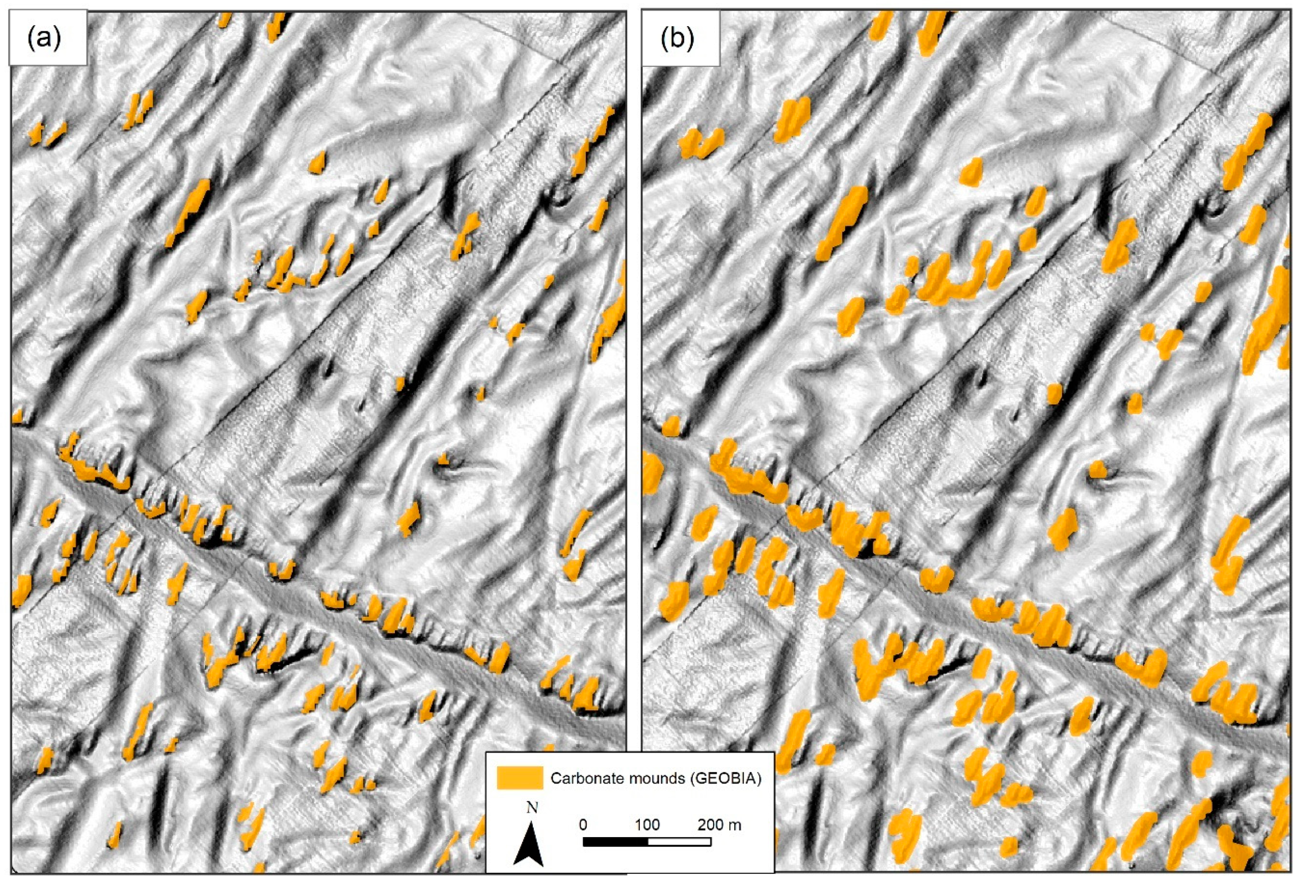
  • Buffering polygons: A BPI-based method of identifying elevated structures will predominantly highlight the highest elevations. By adding a 10-m buffer zone, we aim to include the whole area of each mound feature in the study area (Figure 5). The size of the buffer was selected after trials and visual assessment of the results.
  • Removing results based on polygon size: Many false positives in pixel-based classification will be single cells that happen to have a value above the cut-off limit as we would risk missing actual features if we set the cut-off value too high. These can optionally be removed at the polygon stage by deleting polygons that are smaller than a specified size (700 m2).

2.4. GEOBIA

In GEOBIA, a crucial first step is image segmentation [37,38], in which the image is divided into non-overlapping polygons (objects) in image space based on homogeneity [39] in order to minimize heterogeneity within image objects [25]. These objects are the main analysis units, which make object-based classification fundamentally different from pixel-based methods. The resulting image objects can be characterized by various features, such as layer values (mean, standard deviation, skewness, etc.), geometry (extent, shape, etc.) and image texture. The subsequent classification is based on combinations of these image object features. This can be performed by systematically applying rules that formulate the analyst’s understanding of the image or in a data-driven way through supervised classification (e.g. machine learning). Here, rule-based classification was performed. All rule set parameters were selected following trials and visual assessment of the results. We used eCognition software v9.2 for GEOBIA analysis. The workflow is summarized below and in Figure 6.
  • Segmentation: all bathymetric derivatives were imported to eCognition [32] and segmented using the multiresolution segmentation with a scale parameter of 5 and composition of homogeneity criterion compactness of 0.1. A weighting of 2 was given to BPI5, BPI20, slope and curvature, while 1 was given to the second order polynomial transformation.
  • Classification: a rule-based classification of the objects was performed. The following rules were applied: mean value of BPI5 and BPI20 ≥ 0, mean slope ≥ 5, standard deviation of the slope ≥ 2.3 and standard deviation of curvature ≥ 20.
  • Export to ArcGIS: the classified data were exported to an ArcGIS shapefile as a smoothed polygon.
  • Buffering polygons: A 5-m buffer was applied around the classified polygons with the aim to include the lower parts of carbonate mounds. The size of the buffer was selected after trials and visual assessment of the results (Figure 7).

2.5. Reference Data and Accuracy Assessment

Estimating the accuracies of the three map outputs involves three elements: sampling design, response design and analysis of map accuracy [40,41].

2.5.1. Sampling Design

We selected a stratified-random sampling design with the maximum extent of carbonate mounds (as derived by merging all three outputs) and the absence of mounds as the two strata. Stratified random sampling is a recommended practical design that satisfies the basic accuracy assessment objectives [40]. The sample size was estimated according to the following formula [40,42]:
n = ( W i S i ) 2 [ S ( O ^ ) ] 2 + ( 1 / N ) W i S i 2
where N is the number of units in the region of interest, S ( O ^ ) is the standard error of the estimated overall accuracy that we would like to achieve, Wi is the mapped proportion of area of class i and Si is the standard deviation of stratum i, S i = U i ( 1 U i ) with Ui being the user’s accuracy of class i.

2.5.2. Response Design

Once the reference data points were created (Figure 8), these were labelled by three experts based on a visual assessment of higher-resolution (2 m × 2 m) derivatives (plus surface area to planar area) and shaded relief maps (Figure 1). The reference labelling protocol required the analysts to label the reference points as carbonate mound presence or absence and give a subjective confidence rating (high, moderate, low). Assessments were initially carried out independently. When there was any disagreement between the labels after the initial submission, analysts were asked to find a consensus. The resulting reference data points were used to estimate map accuracies (Figure 1).

2.5.3. Analysis

The predicted classes (mound presence or absence) were attached to the reference data set using a Spatial Join in ArcGIS. Accuracies were analyzed using the function confusionMatrix() of the package caret [43] in R. We assessed the accuracy of the predictions with three widely applied metrics, which can be derived from a contingency table (Table 2). These are namely the overall accuracy (percent classified correctly, PCC), sensitivity and specificity. PCC is the proportion of correctly classified presences and absences (Table 2 and Equation (2)). Sensitivity is the amount of true presence predictions as a proportion of the total number of presence observations (Table 2 and Equation (3)). Specificity is the amount of true absence predictions as a proportion of the total number of absence observations (Table 2 and Equation (4)).
PCC = ( TN + TP ) ( TN + FN + FP + TP )
Sens = TP ( FN + TP )
Spec = TN ( TN + FP )
The statistical significance of the differences in the estimated overall accuracies of the maps was tested with McNemar’s χ2 test for related samples with continuity correction [44]. From the calculated χ2 values and the degrees of freedom (df = 1), a p-value can be derived from published tables or online calculators (e.g., https://www.socscistatistics.com/pvalues/chidistribution.aspx). For a p-value of 0.05, the χ2 value needs to be higher than 3.84.

3. Results

3.1. Reference Data

The maximum extent of carbonate mounds accounted for was 12.3% of the total area and hence, the absence of mounds had a relative area of 87.7%. The number of units in the study area was 3271 individual polygons. Based on previous experience [45], we estimated user accuracies of 0.9 for the mound presence and 0.85 for mound absence. We specified a target standard error for an overall accuracy of 0.02. Hence, we estimated a sample size of 303 according to Equation (1). A proportional allocation of sample points would have resulted in 37 samples for mound presence and 266 for mound absence. To allow for a sufficient number of samples for mound presence, we allocated 100 sample points to this class and the remainder (203) to the mound absence class.
The class labels assigned independently by the three analysts agreed in 280 out of 303 cases (92.4%). When there was disagreement, the confidence in the labelling was typically rated as low or moderate. After a consensus was reached in undecided cases, 73 sample points were labelled as mound presence and 230 as mound absence, leading to a prevalence of 0.24 and a no-information rate (NIR) of 0.76 (Table 3).

3.2. Map Accuracy

Based on the reference dataset, we estimated the map accuracies of the three different approaches (Table 4). All methods achieved overall accuracies (PCC) above the no-information rate (NIR = 0.759). Differences in PCC were small, ranging from 91.09% (manual) to 89.11% (terrain analysis) to 88.45% (GEOBIA). Furthermore, the 95% confidence intervals overlapped (Figure 9). In fact, differences in PCC were not significant based on McNemar’s χ2 test for related samples with continuity correction (Table 5).
The sensitivity was highest for the terrain analysis with 80.82% and lowest for GEOBIA with 64.38%. On the other hand, specificity was highest with 96.09% for both manual and GEOBIA classification.

3.3. Spatial Comparison

Manual digitalization produced 3559 polygons (Table 6). The semi-automated classification based on pixel-based analysis resulted in 3247 polygons, while GEOBIA gave 4866 features. The mapped carbonate mound areas amounted to 6.01 km2, 7.35 km2 and 5.01 km2 for manual mapping, terrain analysis and GEOBIA, respectively. A comparison of the different map outputs is shown in Figure 10.

4. Discussion

We have presented three different methods (manual digitization, pixel-based terrain analysis and object-based image analysis) for classifying carbonate mounds from 5-m grid bathymetry and its derivatives and estimated the map accuracies based on a reference dataset. We selected two rule-based methods (one pixel-based, the other object-based) as they allow for an easier incorporation of the analyst’s understanding of the image and contextual information. More recently, machine learning and deep learning methods have been adopted in image analysis. Such data-driven classification methods hold promise and have been shown to be applicable to CWC carbonate mound mapping [25]. However, results are highly dependent on the quality of the data available for mapping, which can still be a limiting factor in marine mapping applications. Furthermore, the incorporation of the analyst’s knowledge, which is often necessary when data quality issues must be overcome, is more complicated. Therefore, while it would be interesting to further investigate the performance of advanced data-driven classification methods, this is beyond the scope of this paper. Besides, all methods applied in this study achieved high overall accuracies of approximately 90%. Differences between methods in accuracy were small and statistically not significant.
To our knowledge, the method used to derive a reference dataset is novel in marine mapping. Typically, direct observations of the seafloor with underwater videos and still images or physical samples taken with grabs and corers are used as reference data. However, these are often costly to retrieve and analyze and hence limited in number. In this case, we decided to create a reference dataset by directly analyzing high-resolution multibeam echosounder bathymetry data. The process of creating a reference dataset has to be of higher quality than the map-making process [40]. Here, we used the same MBES data gridded to a finer resolution (2 m vs 5 m) and the consensual labelling from three analysts to produce a reference dataset. Thus, we deem the reference labelling process to be of higher quality than the map-making processes. This approach is viable here because carbonate mounds are well-recognizable features to a skilled analyst. To limit uncertainty in the reference data, we applied a reference labelling protocol that minimized interpreter variability. From the results, it is obvious that the inter-analyst variability is low as the reference points were labelled differently in only 8% of cases. This occurred most frequently in transition areas at the bottom of mound slopes. The low disagreement is likely due to (1) the fact that carbonate mounds are conspicuous features readily identifiable from MBES data [25] and (2) the use of a simple binary (presence/absence) classification [46].
The reference labelling approach we have taken has several advantages. There is no geolocation error in the reference dataset as the labelling is based on the same MBES data (albeit processed to a higher resolution) as the data used for mapping. Likewise, there are no temporal mismatches as the data used for mapping and deriving the reference dataset are of the same age. Most importantly, the reference dataset could be created cheaply and quickly (within a day), which allowed us to follow recommendations for appropriate sample size and sampling design [40,41]. This is in contrast with data partitioning, in which one set of ground-truth data points is split into training and testing datasets [47]. Such an approach is frequently conducted when it is not possible to specifically collect independent ground-truth data in a separate survey after map production. It does, however, invariably mean that it is not possible to apply well-established recommendations for sampling design. As a result, such single splits into training and testing data frequently lead to high variance in estimates of accuracy [48] although this problem might be alleviated by applying bootstrap aggregation [45].
There was little difference in the overall map accuracy between the three methods. However, differences were more pronounced in terms of sensitivity and specificity. With the parameters used in this study, the terrain analysis method was most successful in predicting the presence of mounds (highest sensitivity) and predicting the largest carbonate mound area (Table 5). GEOBIA and manual classification were superior in the identification of the absence of mounds (highest specificity) in line with smaller predicted areas of carbonate mounds when compared with terrain analysis. Choosing the most appropriate mapping method will not only depend on these differences in error statistics but also on the task in hand. If the requirement is to correctly classify as many carbonate mounds as possible, our results suggest that terrain analysis might be the method of choice. However, if the task is to minimize the number of false positives, it might be more appropriate to utilize GEOBIA or manual interpretation (Table 7).
The number of produced mound polygons varies from 3247 to 4866. Dependent on the mapping scale, manual mapping will lead to generalizations, in which individual carbonate mounds might be grouped together when in close proximity. The lower number of polygons resulting from the terrain analysis when compared with GEOBIA is likely a result of the larger buffer size (10 m vs. 5 m), which was chosen separately for each method with the aim to improve mapping performance (as judged by the analyst). Whether it is necessary to map individual carbonate mounds as precisely as possible or some generalization is acceptable will depend on the usage of the map products. Taken together, this indicates that a “one size fits all” mapping approach is unlikely to exist, and it will be important to first specify map requirements based on anticipated usage as precisely as possible before choosing the most appropriate method. Trade-offs (e.g., favoring high sensitivity over high specificity) will be unavoidable.
The statistically insignificant differences in overall accuracy indicate that semi-automated rule-based methods can reliably substitute time-consuming and subjective manual methods. The mapped area of this case study was small (76 km2) when compared with the size of the Norwegian continental shelf (≈1,400,000 km2) or the area suitable for CWC growth (≈1,000,000 km2) therein [8]. Such large areas can only be mapped manually with increased generalization (decreased mapping scale) as has been done previously [26]. To maintain the level of detail contained in 5-m MBES data will require some level of automation and as showcased here, rule-based methods are a viable option. The GEOBIA rule-set is now developed and tested. However, the parameters potentially need to be tuned if applied in a new study area. The same applies for the terrain analysis method with the work flow defined but it will take some iterations to obtain satisfactory results or create a model with Model Builder. The map accuracy can be reliably assessed by producing reference datasets through labelling by experts. Ultimately, this means that the expertise of involved analysts is still needed but the focus will shift from manual map production to the creation of reference data. In this way, it should be possible to map large areas of the seabed with high spatial resolution and to assess and critically evaluate the accuracy of the derived products. Such products are likely to improve the database for spatial management and conservation. Estimates of carbonate mound area might also help to constrain the rate of carbonate production of CWC reefs [8] and their role as carbonate sinks [7].

5. Conclusions

Two semi-automated rule-based methods (pixel-based terrain analysis and GEOBIA) were compared with manual mapping in their ability to accurately map CWC carbonate mounds based on high-resolution MBES bathymetry data. To test the accuracy of the methods, we created a reference dataset by selecting 303 points in a stratified random way. These points were subsequently classified as carbonate mound presence or absence by three expert analysts. Based on the reference data, we estimated map accuracy and found that all methods produced highly accurate results with an overall accuracy of approximately 90%. Moreover, there were no statistically significant differences in those accuracy values, meaning that more time-efficient semi-automated methods can replace laborious manual mapping in the future. Application of such methods in seafloor mapping programs will likely increase the evidence base for sustainable management and conservation.

Author Contributions

Conceptualization, A.J., T.T. and M.D.; Methodology, A.J., N.J.B., S.E., and M.D.; Software, A.J., N.J.B., S.E., V.K.B. and M.D.; Validation, A.J. and M.D.; Formal analysis, A.J., N.J.B., S.E., V.K.B. and M.D.; Investigation, A.J., T.T. and M.D.; Resources, A.J., N.J.B., S.E., T.T. and M.D.; Data curation, A.J. and M.D.; Writing—original draft preparation, A.J., N.J.B., S.E. and T.T.; Writing—review & editing, A.J., N.J.B., S.E., V.K.B. and M.D.; Visualization, A.J. and M.D.; Supervision, M.D.; Project administration, T.T.

Funding

This research received no external funding. This study was funded by the Geological Survey of Norway.

Acknowledgments

The bathymetry data were made available by the Norwegian Mapping Authority, funded by the MAREANO program. We would like to acknowledge Kartverket (the Norwegian Hydrographic Service) and the MAREANO programme for the provision of the bathymetry dataset, used here under a CC by 4.0 license (https://creativecommons.org/licenses/by/4.0/legalcode).

Conflicts of Interest

The authors declare no conflict of interest. The funders had no role in the design of the study; in the collection, analyses, or interpretation of data; in the writing of the manuscript, or in the decision to publish the results.

References

  1. Roberts, J.M.; Wheeler, A.J.; Freiwald, A. Reefs of the Deep: The Biology and Geology of Cold-Water Coral Ecosystems. Science 2006, 312, 543–547. [Google Scholar] [CrossRef] [PubMed]
  2. Bongiorni, L.; Mea, M.; Gambi, C.; Pusceddu, A.; Taviani, M.; Danovaro, R. Deep-water scleractinian corals promote higher biodiversity in deep-sea meiofaunal assemblages along continental margins. Biol. Conserv. 2010, 143, 1687–1700. [Google Scholar] [Green Version]
  3. Baillon, S.; Hamel, J.F.; Wareham, V.E.; Mercier, A. Deep cold-water corals as nurseries for fish larvae. Front. Ecol. Environ. 2012, 10, 351–356. [Google Scholar] [CrossRef]
  4. Söffker, M.; Sloman, K.A.; Hall-Spencer, J.M. In situ observations of fish associated with coral reefs off Ireland. Deep. Res. Part I Oceanogr. Res. Pap. 2011, 58, 818–825. [Google Scholar] [CrossRef] [Green Version]
  5. Costello, M.J.; McCrea, M.; Freiwald, A.; Lundälv, T.; Jonsson, L.; Bett, B.J.; van Weering, T.C.E.; de Haas, H.; Roberts, J.M.; Allen, D. Role of cold-water Lophelia pertusa coral reefs as fish habitat in the NE Atlantic. In Cold-Water Corals and Ecosystems; Springer: Berlin, Heidelberg, 2005; pp. 771–805. [Google Scholar]
  6. Hoegh-Guldberg, O.; Poloczanska, E.S.; Skirving, W.; Dove, S. Coral Reef Ecosystems under Climate Change and Ocean Acidification. Front. Mar. Sci. 2017, 4. [Google Scholar] [CrossRef] [Green Version]
  7. Titschack, J.; Baum, D.; De Pol-Holz, R.; López Correa, M.; Forster, N.; Flögel, S.; Hebbeln, D.; Freiwald, A. Aggradation and carbonate accumulation of Holocene Norwegian cold-water coral reefs. Sedimentology 2015, 62, 1873–1898. [Google Scholar] [CrossRef]
  8. Lindberg, B.; Mienert, J. Postglacial carbonate production by cold-water corals on the Norwegian Shelf and their role in the global carbonate budget. Geology 2005, 33, 537–540. [Google Scholar] [CrossRef]
  9. Althaus, F.; Williams, A.; Schlacher, T.; Kloser, R.J.; Green, M.; Barker, B.; Bax, N.; Brodie, P. Impacts of bottom trawling on deep-coral ecosystems of seamounts are long-lasting. Mar. Ecol. Prog. Ser. 2009, 397, 279–294. [Google Scholar] [CrossRef] [Green Version]
  10. Hall–Spencer, J.; Allain, V.; Fosså, J.H. Trawling damage to Northeast Atlantic ancient coral reefs. Proc. R. Soc. London. Ser. B Biol. Sci. 2002, 269, 507–511. [Google Scholar] [CrossRef] [Green Version]
  11. Fosså, J.H.; Mortensen, P.B.; Furevik, D.M. The deep-water coral Lophelia pertusa in Norwegian waters: Distribution and fishery impacts. Hydrobiologia 2002, 471, 1–12. [Google Scholar] [CrossRef]
  12. Roberts, J.M.; Cairns, S.D. Cold-water corals in a changing ocean. Curr. Opin. Environ. Sustain. 2014, 7, 118–126. [Google Scholar] [CrossRef] [Green Version]
  13. Fisher, C.R.; Hsing, P.-Y.; Kaiser, C.L.; Yoerger, D.R.; Roberts, H.H.; Shedd, W.W.; Cordes, E.E.; Shank, T.M.; Berlet, S.P.; Saunders, M.G.; Larcom, E.A.; Brooks, J.M. Footprint of Deepwater Horizon blowout impact to deep-water coral communities. Proc. Natl. Acad. Sci. 2014, 111, 11744–11749. [Google Scholar] [CrossRef] [PubMed] [Green Version]
  14. Torrents, O.; Tambutté, E.; Caminiti, N.; Garrabou, J. Upper thermal thresholds of shallow vs. deep populations of the precious Mediterranean red coral Corallium rubrum (L.): Assessing the potential effects of warming in the NW Mediterranean. J. Exp. Mar. Bio. Ecol. 2008, 357, 7–19. [Google Scholar] [CrossRef]
  15. Guinotte, J.M.; Orr, J.; Cairns, S.; Freiwald, A.; Morgan, L.; George, R. Will human-induced changes in seawater chemistry alter the distribution of deep-sea scleractinian corals? Front. Ecol. Environ. 2006, 4, 141–146. [Google Scholar] [CrossRef]
  16. Dullo, W.-C.; Flögel, S.; Rüggeberg, A. Cold-water coral growth in relation to the hydrography of the Celtic and Nordic European continental margin. Mar. Ecol. Prog. Ser. 2008, 371, 165–176. [Google Scholar] [CrossRef] [Green Version]
  17. Kiriakoulakis, K.; Freiwald, A.; Fisher, E.; Wolff, G.A. Organic matter quality and supply to deep-water coral/mound systems of the NW European Continental Margin. Int. J. Earth Sci. 2007, 96, 159–170. [Google Scholar] [CrossRef]
  18. Edinger, E.N.; Sherwood, O.A.; Piper, D.J.W.; Wareham, V.E.; Baker, K.D.; Gilkinson, K.D.; Scott, D.B. Geological features supporting deep-sea coral habitat in Atlantic Canada. Cont. Shelf Res. 2011, 31, 69–84. [Google Scholar] [CrossRef]
  19. Thorsnes, T.; Bellec, V.K.; Dolan, M.F.J. Cold-water coral reefs and glacial landforms from Sula Reef, mid-Norwegian shelf. Geol. Soc. London, Mem. 2016, 46, 307–308. [Google Scholar] [CrossRef]
  20. Buhl-Mortensen, L.; Vanreusel, A.; Gooday, A.J.; Levin, L.A.; Priede, I.G.; Buhl-Mortensen, P.; Gheerardyn, H.; King, N.J.; Raes, M. Biological structures as a source of habitat heterogeneity and biodiversity on the deep ocean margins. Mar. Ecol. 2010, 31, 21–50. [Google Scholar] [CrossRef] [Green Version]
  21. Freiwald, A.; Rogers, A.; Hall-Spencer, J.; Guinotte, J.; Davies, A.; Yesson, C.; Martin, C.; Weatherdon, L. Global distribution of cold-water corals (version 5.0). Fifth update to the dataset in Freiwald et al. (2004) by UNEP-WCMC, in collaboration with Andre Freiwald and John Guinotte.
  22. Anderson, O.F.; Guinotte, J.M.; Rowden, A.A.; Clark, M.R.; Mormede, S.; Davies, A.J.; Bowden, D.A. Field validation of habitat suitability models for vulnerable marine ecosystems in the South Pacific Ocean: Implications for the use of broad-scale models in fisheries management. Ocean Coast. Manag. 2016, 120, 110–126. [Google Scholar] [CrossRef] [Green Version]
  23. Wheeler, A.J.; Beyer, A.; Freiwald, A.; de Haas, H.; Huvenne, V.A.I.; Kozachenko, M.; Olu-Le Roy, K.; Opderbecke, J. Morphology and environment of cold-water coral carbonate mounds on the NW European margin. Int. J. Earth Sci. 2007, 96, 37–56. [Google Scholar] [CrossRef]
  24. De Clippele, L.H.; Gafeira, J.; Robert, K.; Hennige, S.; Lavaleye, M.S.; Duineveld, G.C.A.; Huvenne, V.A.I.; Roberts, J.M. Using novel acoustic and visual mapping tools to predict the small-scale spatial distribution of live biogenic reef framework in cold-water coral habitats. Coral Reefs 2017, 36, 255–268. [Google Scholar] [CrossRef]
  25. Diesing, M.; Thorsnes, T. Mapping of Cold-Water Coral Carbonate Mounds Based on Geomorphometric Features: An Object-Based Approach. Geosciences 2018, 8, 34. [Google Scholar] [CrossRef]
  26. Bellec, V.K.; Thorsnes, T.; Bøe, R. Mapping of bioclastic sediments - data, methods and confidence. NGU-rapport 2014, 2014.006, 23. [Google Scholar]
  27. Freiwald, A.; Hühnerbach, V.; Lindberg, B.; Wilson, J.B.; Campbell, J. The Sula Reef Complex, Norwegian shelf. Facies 2002, 47, 179–200. [Google Scholar] [CrossRef]
  28. Bellec, V.K.; Bøe, R.; Rise, L.; Lepland, A.; Thorsnes, T.; Bjarnadóttir, L.R. Seabed sediments (grain size) of Nordland VI, offshore north Norway. J. Maps 2017, 13, 608–620. [Google Scholar] [CrossRef]
  29. Wright, D.J.; Pendleton, M.; Boulware, J.; Walbridge, S.; Gerlt, B.; Eslinger, D.; Sampson, D.H.E. Unified Geomorphological Analysis Workflows with Benthic Terrain Modeler. Geosciences 2018, 8, 94. [Google Scholar] [CrossRef]
  30. Li, J.; Heap, A.D.; Potter, A.; Huang, Z.; Daniell, J.J. Can we improve the spatial predictions of seabed sediments? A case study of spatial interpolation of mud content across the southwest Australian margin. Cont. Shelf Res. 2011, 31, 1365–1376. [Google Scholar] [CrossRef]
  31. Huang, Z.; Siwabessy, J.; Nichol, S.; Anderson, T.; Brooke, B. Predictive mapping of seabed cover types using angular response curves of multibeam backscatter data: Testing different feature analysis approaches. Cont. Shelf Res. 2013, 61–62, 12–22. [Google Scholar] [CrossRef]
  32. eCognition eCognition Developer 9. Available online: http://www.ecognition.com/suite/ecognition-developer (accessed on 10 May 2018).
  33. Wilson, M.F.J.; O’Connell, B.; Brown, C.; Guinan, J.C.; Grehan, A.J. Multiscale terrain analysis of multibeam bathymetry data for habitat mapping on the continental slope. Mar. Geod. 2007, 30, 3–35. [Google Scholar]
  34. Lundblad, E.R.; Wright, D.J.; Miller, J.; Larkin, E.M.; Rinehart, R.; Naar, D.F.; Donahue, B.T.; Anderson, S.M.; Battista, T. A Benthic Terrain Classification Scheme for American Samoa. Mar. Geod. 2006, 29, 89–111. [Google Scholar] [CrossRef]
  35. ArcGIS Pro Overview of georeferencing. Available online: http://pro.arcgis.com/en/pro-app/help/data/imagery/overview-of-georeferencing.htm (accessed on 27 September 2018).
  36. Jakobsson, M.; Gyllencreutz, R.; Mayer, L.A.; Dowdeswell, J.A.; Canals, M.; Todd, B.J.; Dowdeswell, E.K.; Hogan, K.A.; Larter, R.D. Mapping submarine glacial landforms using acoustic methods. Geol. Soc. London, Mem. 2016, 46, 17–40. [Google Scholar] [CrossRef] [Green Version]
  37. Blaschke, T.; Hay, G.J.; Kelly, M.; Lang, S.; Hofmann, P.; Addink, E.; Queiroz Feitosa, R.; van der Meer, F.; van der Werff, H.; van Coillie, F.; Tiede, D. Geographic Object-Based Image Analysis—Towards a new paradigm. ISPRS J. Photogramm. Remote Sens. 2014, 87, 180–191. [Google Scholar] [CrossRef] [PubMed]
  38. Hay, G.J.; Castilla, G. Geographic Object-Based Image Analysis (GEOBIA): A new name for a new discipline. In Object-Based Image Analysis: Spatial Concepts for Knowledge-Driven Remote Sensing Applications; Blaschke, T., Lang, S., Hay, G.J., Eds.; Springer: Berlin, Germany, 2008; pp. 75–89. [Google Scholar]
  39. Schiewe, J. Segmentation of high-resolution remotely sensed data—Concepts, applications and problems. In Proceedings of the Symposium on Geospatial theory, Processing and Applications, Ottawa, ON, Canada, 9–12 July 2002. [Google Scholar]
  40. Olofsson, P.; Foody, G.M.; Herold, M.; Stehman, S.V.; Woodcock, C.E.; Wulder, M.A. Good practices for estimating area and assessing accuracy of land change. Remote Sens. Environ. 2014, 148, 42–57. [Google Scholar] [CrossRef] [Green Version]
  41. Stehman, S.V.; Czaplewski, R.L. Design and Analysis for Thematic Map Accuracy Assessment—An application of satellite imagery. Remote Sens. Environ. 1998, 64, 331–344. [Google Scholar] [CrossRef]
  42. Cochran, W.G. Sampling techniques, 3rd ed.; John Wiley & Sons: New York, NY, USA, 1977. [Google Scholar]
  43. Kuhn, M. Building Predictive Models in R Using the caret Package. J. Stat. Software 2008, 28, 1–26. [Google Scholar] [CrossRef]
  44. Foody, G.M. Thematic Map Comparison: Evaluating the Statistical Significance of Differences in Classification Accuracy. Photogramm. Eng. Remote Sens. 2004, 70, 627–633. [Google Scholar] [CrossRef]
  45. Mitchell, P.J.; Downie, A.-L.; Diesing, M. How good is my map? A tool for semi-automated thematic mapping and spatially explicit confidence assessment. Environ. Model. Softw. 2018, 108, 111–122. [Google Scholar] [CrossRef]
  46. Rattray, A.J.; Ierodiaconou, D.; Monk, J.; Laurenson, L.; Kennedy, P. Quantification of Spatial and Thematic Uncertainty in the Application of Underwater Video for Benthic Habitat Mapping. Mar. Geod. 2014, 37, 315–336. [Google Scholar] [CrossRef]
  47. Fielding, A.H.; Bell, J.F. A review of methods for the assessment of prediction errors in conservation presence/absence models. Environ. Conserv. 1997, 24, 38–49. [Google Scholar] [CrossRef]
  48. Lyons, M.B.; Keith, D.A.; Phinn, S.R.; Mason, T.J.; Elith, J. A comparison of resampling methods for remote sensing classification and accuracy assessment. Remote Sens. Environ. 2018, 208, 145–153. [Google Scholar] [CrossRef]
Figure 1. Flowchart summarizing the experiment.
Ijgi 08 00040 g001
Figure 2. (a) Location of study area located on Skjoldryggen on the Mid-Norwegian continental shelf. (b) Close-up of study area; also shown are bioclastic sediments mapped by the MAREANO program as a proxy for CWC carbonate mounds [26]. (c) Area presented later in Figures 4 and 5. (d) Area presented later in Figure 3. (e) Area presented later in Figure 8. Elongated carbonate mounds can be seen growing in a NW–SE direction on a surface furrowed by iceberg plough marks (ce).
Ijgi 08 00040 g002
Figure 3. Different derivatives overlaid by manually mapped carbonate mounds (in green): (a) BPI20, (b) slope, (c) plan curvature and (d) profile curvature.
Ijgi 08 00040 g003
Figure 4. Flowchart summarizing the process of pixel-based terrain analysis.
Ijgi 08 00040 g004
Figure 5. Classified polygons based on BPI3. (a) Classified polygons without buffer. (b) Classified polygons after applying 10-m buffer zone.
Ijgi 08 00040 g005
Figure 6. Flowchart summarizing the process of GEOBIA.
Ijgi 08 00040 g006
Figure 7. (a) Close-up of the semi-automatic classification exported from eCognition and (b) close-up result of semi-automatic classification with 5-m buffer in orange used for comparison.
Ijgi 08 00040 g007
Figure 8. (a) The distribution of reference points in the whole study area. (b) Example with definition of mounds based on merging all 3 classifications into one for random selection of reference points dataset.
Ijgi 08 00040 g008
Figure 9. Comparison of overall accuracy (PCC) mean (dot) and 95% confidence intervals (whiskers) for the three methods.
Ijgi 08 00040 g009
Figure 10. Area showing the distribution of reference points and overlapping of all three classifications together with bioclastic sediments [26].
Ijgi 08 00040 g010
Table 1. Bathymetric derivates utilized in the study.
DerivativeDescriptionReference
Slope [°]The maximum slope gradient.[33]
CurvatureThe rate of change of slope.[33]
Profile and plan curvatureProfile curvature is measured parallel to the slope, plan curvature perpendicular.[33]
Bathymetric positioning
index (BPI) [m]
Vertical position of a cell relative to its neighborhood.[34]
Surface area to Planar area *Computes a ratio between the three-dimensional surface area and the planar area of the surface.[29]
Second order polynomial transformation *Creates bend or curved adjusted transformation of the dataset[35]
* Derivates only used to produce the reference dataset.
Table 2. Contingency table for presence–absence predictions and selected associated accuracy metrics.
Observed AbsenceObserved Presence
Predicted absenceTrue negative (TN)False negative (FN)
Predicted presenceFalse positive (FP)True positive (TP)
Table 3. Summary of the reference dataset.
No. of ObservationsFractionMeaning
Presence730.241= Prevalence
Absence2300.759= No-information Rate
Sum3031
Table 4. Contingency table for presence–absence predictions with results for 3 classifications. PA, PP, OA and OP denotes predicted absence/presence or observed absence/presence, respectively.
ManualTerrain Analysis GEOBIA
OAOPOAOPOAOP
PA221182111422126
PP9551959947
PCC0.91090.89110.8845
95% CI(0.873, 0.9405)(0.8505, 0.9238)(0.843, 0.9182)
NIR0.75910.75910.7591
P-Value [Acc > NIR]7.40E-124.44E-092.85E-08
Sensitivity0.75340.80820.6438
Specificity0.96090.91740.9609
Table 5. Evaluation of statistical significance of differences in classification accuracy based on McNemar’s χ2 test for related samples with continuity correction. For a p-value of 0.05, the χ2 value needs to be higher than 3.84.
p-values\χ2ManualTerrain AnalysisGEOBIA
manual-0.5211.225
terrain analysis0.471-0.025
GEOBIA0.2680.874-
Table 6. Mapped carbonate mounds expressed as the number of polygons and area by method.
ManualTerrain AnalysisGEOBIA
Number of polygons355932474866
Area (km2)6.017.355.01
Table 7. Comparison of the strengths of the different methods.
MethodManualTerrain AnalysisGEOBIA
Has highestspecificitysensitivityspecificity
Minimizesnumber of false positivesnumber of false negativesnumber of false positives
Best predictsAbsence of moundsPresence of moundsAbsence of mounds

