Dynamic Recommendation of Substitute Locations for Inaccessible Soil Samples during Field Sampling Campaign

 , , , and
Abstract
:1. Introduction
2. Design of the Proposed Method
2.1. Step 1: Selecting Potential Substitute Locations with High Substitutive Scores
- Simple random sampling. If a sample location designed with simple random sampling was inaccessible, its substitute location should also be randomly selected. Thus, the proposed method randomly generates some potential substitute locations (different from those samples in the original sampling plan) in the study area, and assigns each with a substitutive score of 1 as they are equally substitutive. A buffer to other samples in the original sampling plan may be used to prevent the potential substitute locations from being unreasonably close to existing samples. Such a buffer restriction is also available for the rest four situations in this step.
- Stratified random sampling. For an inaccessible sample designed with stratified random sampling, its potential substitute locations should be randomly selected using the same stratifying factor (i.e., with the same class value of the stratified factor) as the inaccessible sample. These potential substitute locations are assigned with a substitutive score of 1.
- Grid sampling. For an inaccessible sample from grid sampling, its potential substitute locations are selected near the inaccessible sample, so that the layout of collected samples can still roughly fit the regular grid adopted in the original design of the grid sampling. It should be as close as possible to the inaccessible sample. The substitutive score of each potential substitute location is calculated as 1 minus the distance between the potential substitute location and the inaccessible sample divided by the grid size.
- Purposive sampling. Purposive sampling is to design samples based on samples’ representativeness of the geographic environment. Sample representativeness is often quantified based on the similarity of environmental conditions between the sample and other locations in the area [4,5,16]. Therefore, for an inaccessible sample from purposive sampling, the substitutive score of a potential substitute location is determined by its environmental similarity to the inaccessible sample. In our method, the environmental similarity is calculated as in Zhu et al. [17], which consists of three steps. The first step is to choose environmental covariates that closely relate to the spatial variation of soils in the study area. Then, the similarity of each individual environmental covariate between two locations (i.e., the inaccessible sample and one of its potential substitute locations) is calculated. If the covariate is nominal or ordinal, the similarity based on this covariate is either 1 or 0. If the covariate is interval or ratio, the similarity is calculated with a Gaussian-shaped curve [17,18]:where is the environmental similarity between two locations, and are the v-th environmental covariate values at location i and j respectively, and is the standard deviation of v-th environmental covariate in the study area. The width of the Gaussian-shaped curve is controlled by to ensure that the curve is reasonably spread over the value range of v-th environmental covariate. The Gaussian-shaped curve assigns high similarity to locations with close covariate values. Finally, the environmental similarity between two locations is assigned to be the minimum among all similarities based on individual environmental covariates, which is based on the limiting factor principle [17,19].
- Unknown or other possible sampling strategies. For other sampling strategies, the approach used to calculate the substitutive score for purposive sampling can be adopted as in Wei [13].
2.2. Step 2: Calculating the Accessibility Score for each Candidate Substitute Location
- The instant sampling scenario. This is when the surveyor plans to collect the substitute sample right away. A lower cost means a shorter distance from the surveyor’s current location to a substitutive location. Under this scenario, the proposed method uses the surveyor’s current location as the source position in the source layer to calculate accumulative costs. If the surveyor’s position is not available, the location of the inaccessible sample will be treated as the source location. Under this scenario, it is assumed that the surveyor would immediately request the substitute location to be identified when a predesigned sample was found to be inaccessible.
- The subsequent sampling scenario. This is when the surveyor plans to collect the substitute sample at a later time during collecting other remaining predesigned samples and not right away. Under this scenario, the big picture of the sampling progress will be considered. The proposed method uses the locations of all uncollected samples as potential sources in the source layer.
2.3. Step 3: Recommending the Final Substitute Sample Location
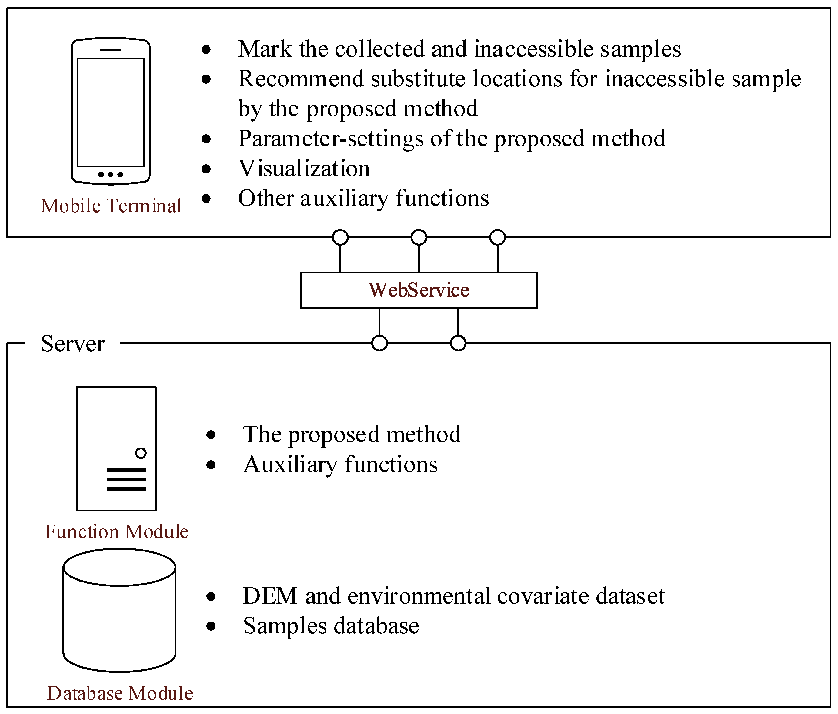
3. The Prototype System
4. Case Study
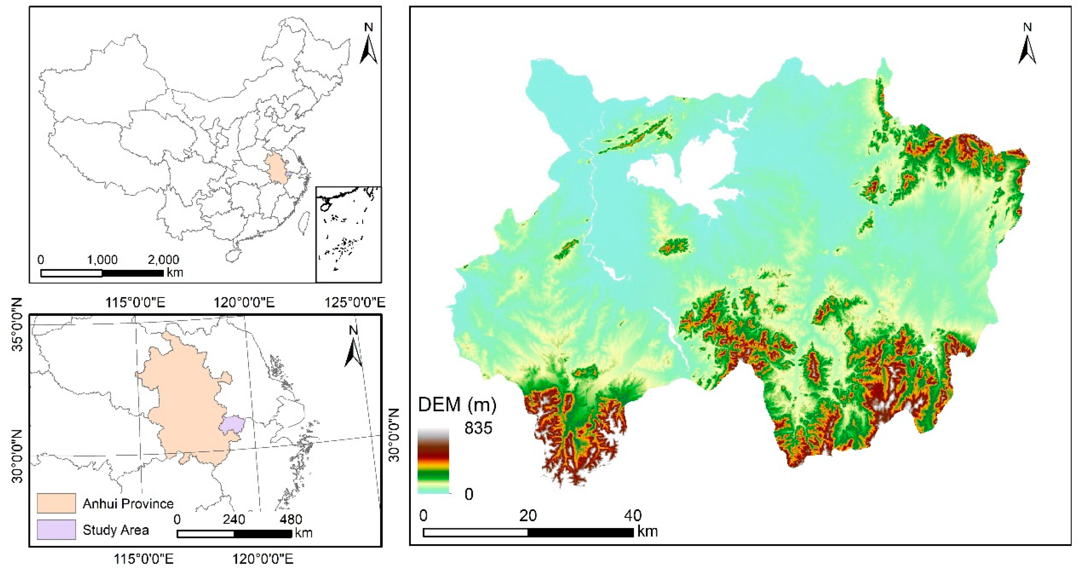
4.1. Study Area
4.2. Data Preparation
4.2.1. Environmental Covariate Data
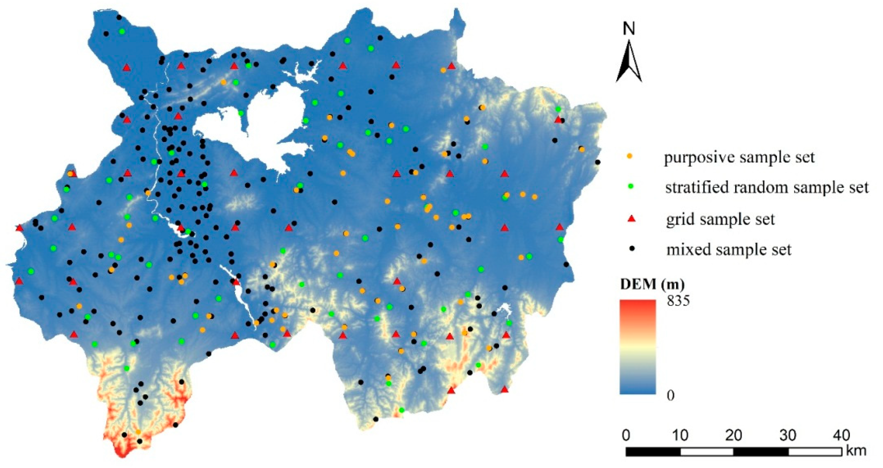
4.2.2. Soil Sample Data
4.2.3. Sampling Cost Layer
4.3. Experimental Design
4.3.1. Evaluating Sampling Scenarios
4.3.2. Evaluating the Quality of Substitute Locations
5. Results and Discussion
5.1. The Two Sampling Scenarios in the Proposed Method
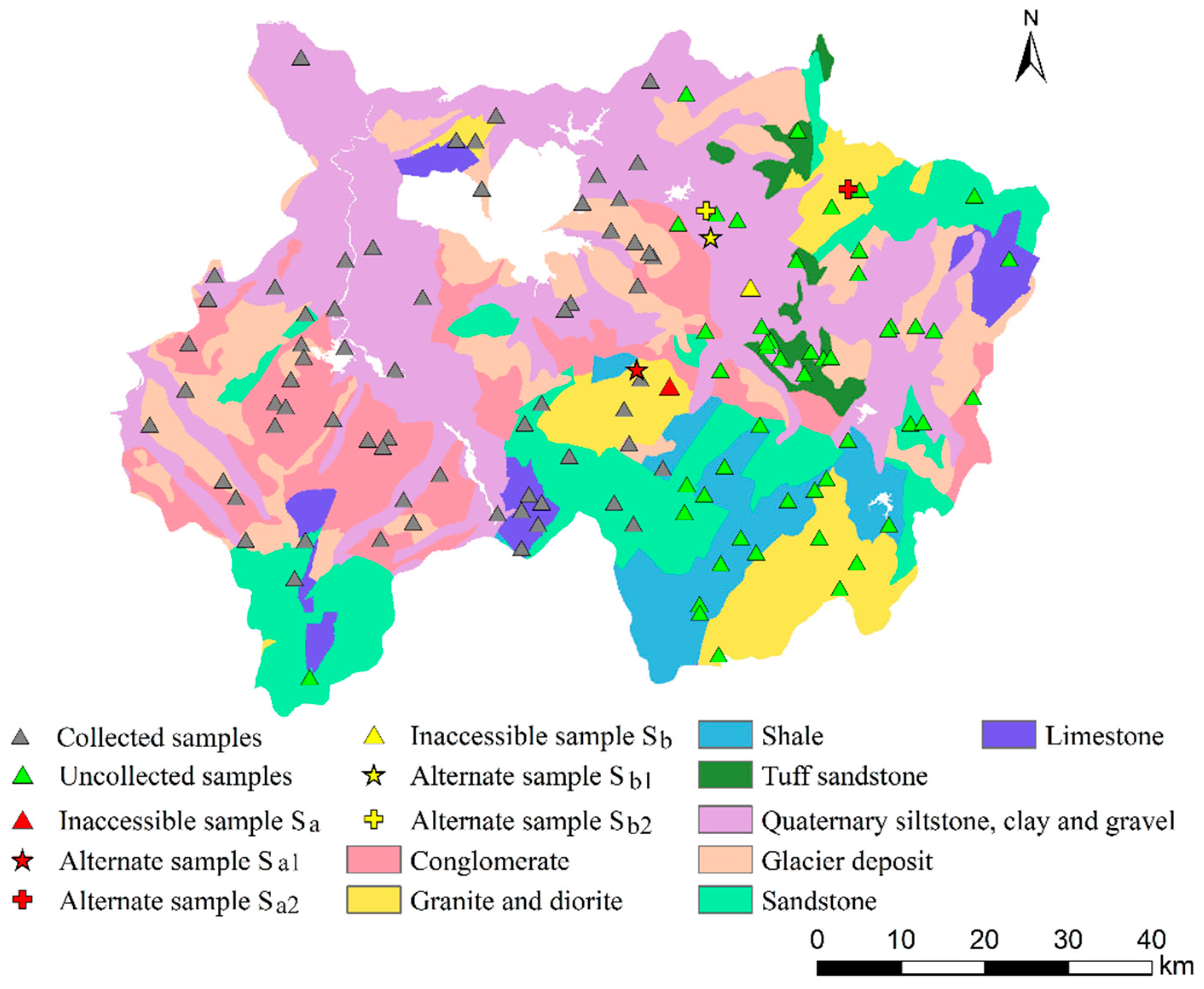
5.2. The Substitute Samples for Purposive Sampling
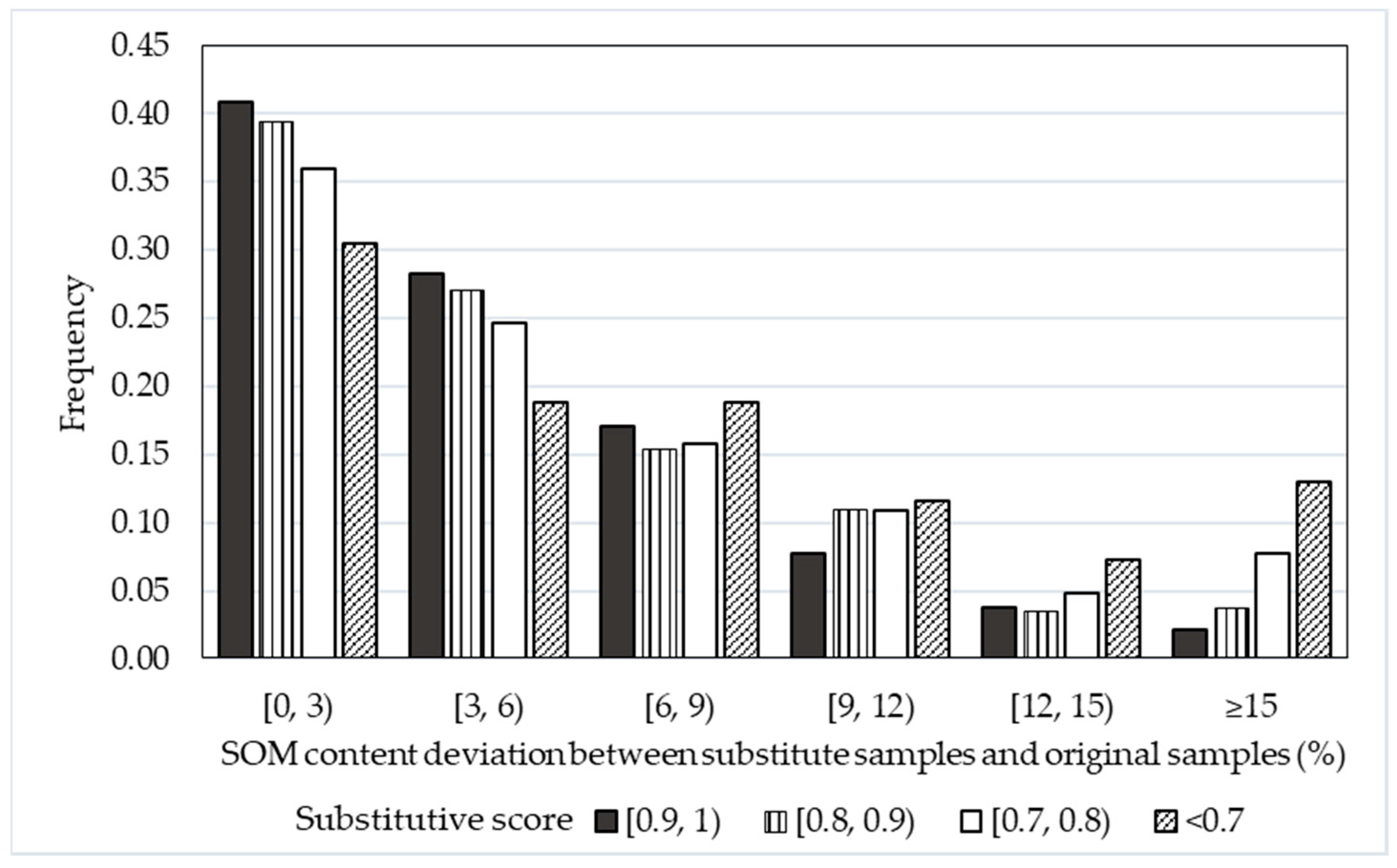
5.2.1. Sample Deviation
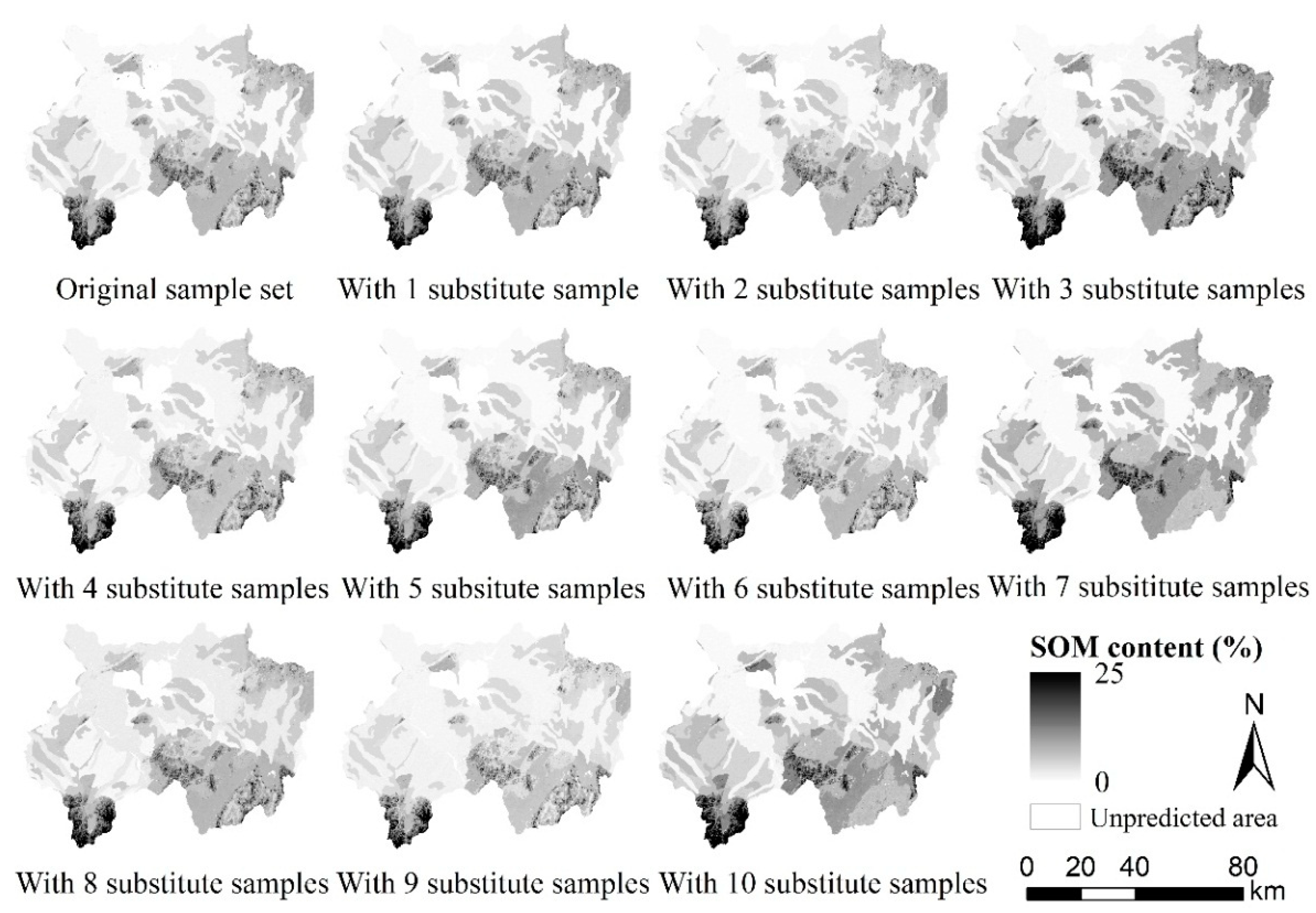
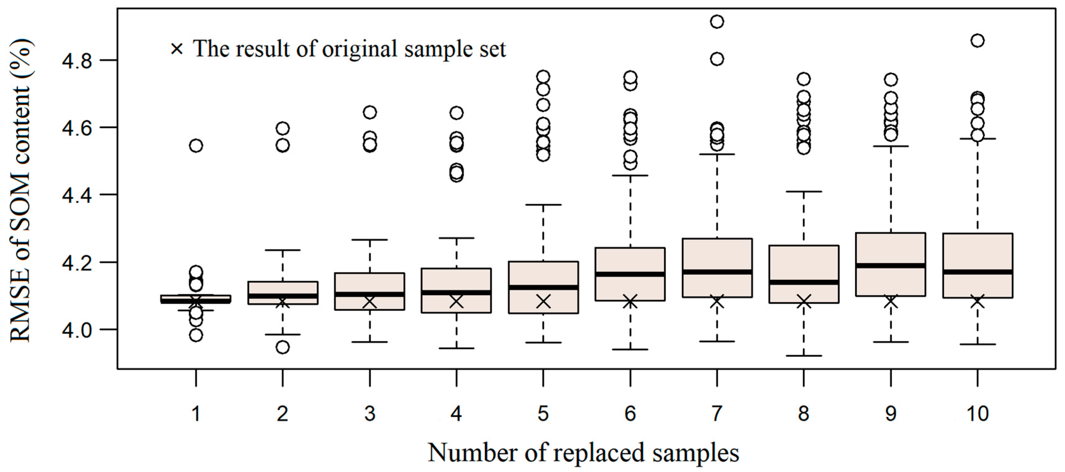
5.2.2. Mapping Accuracy
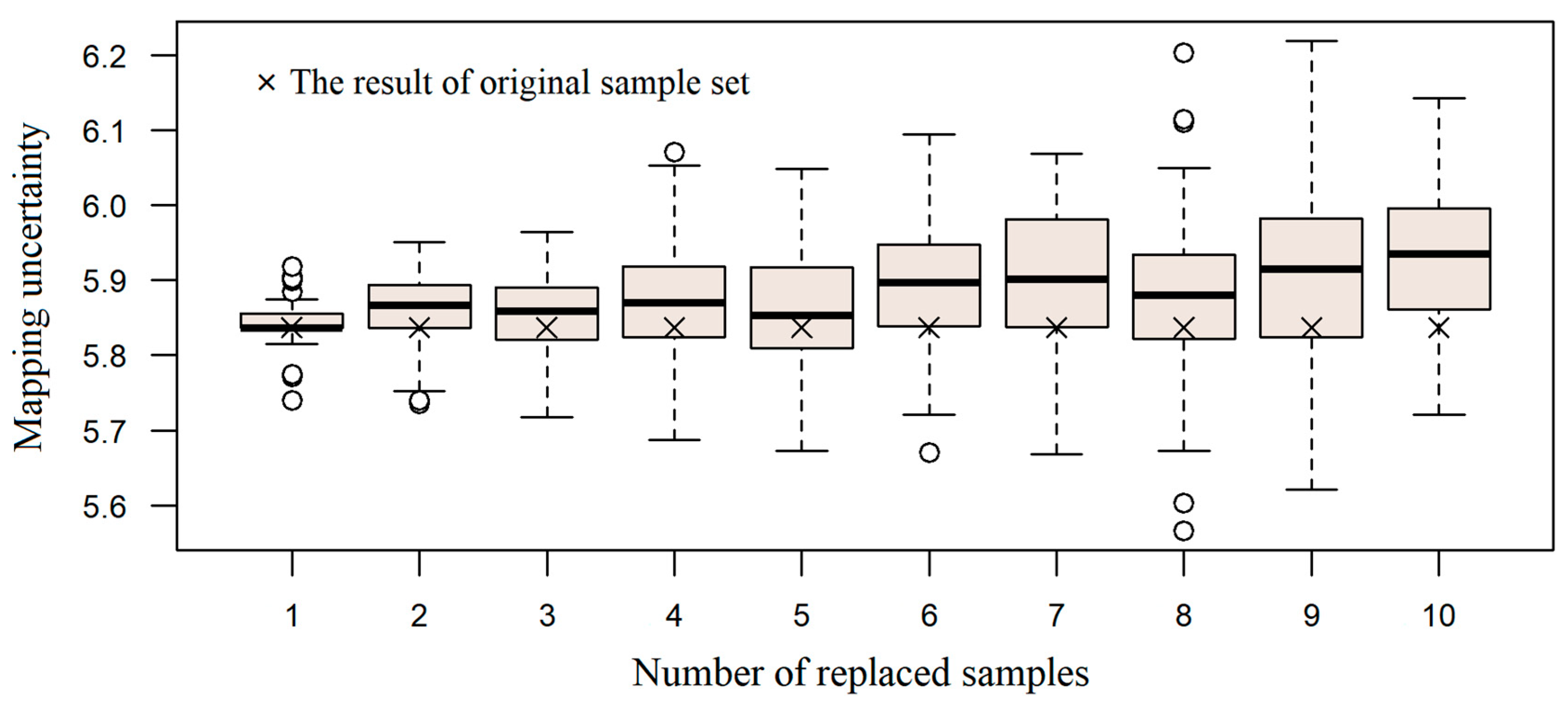
5.2.3. Prediction Uncertainty
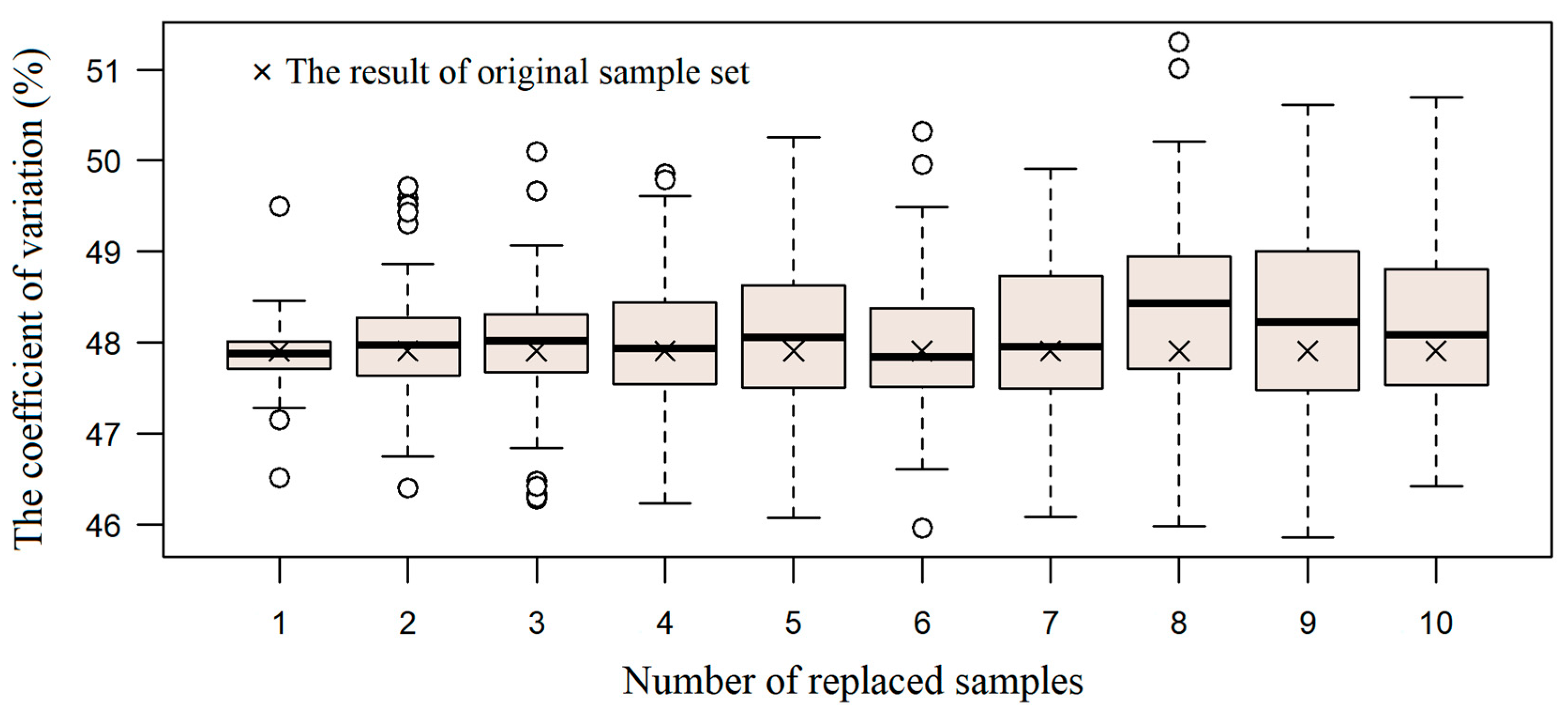
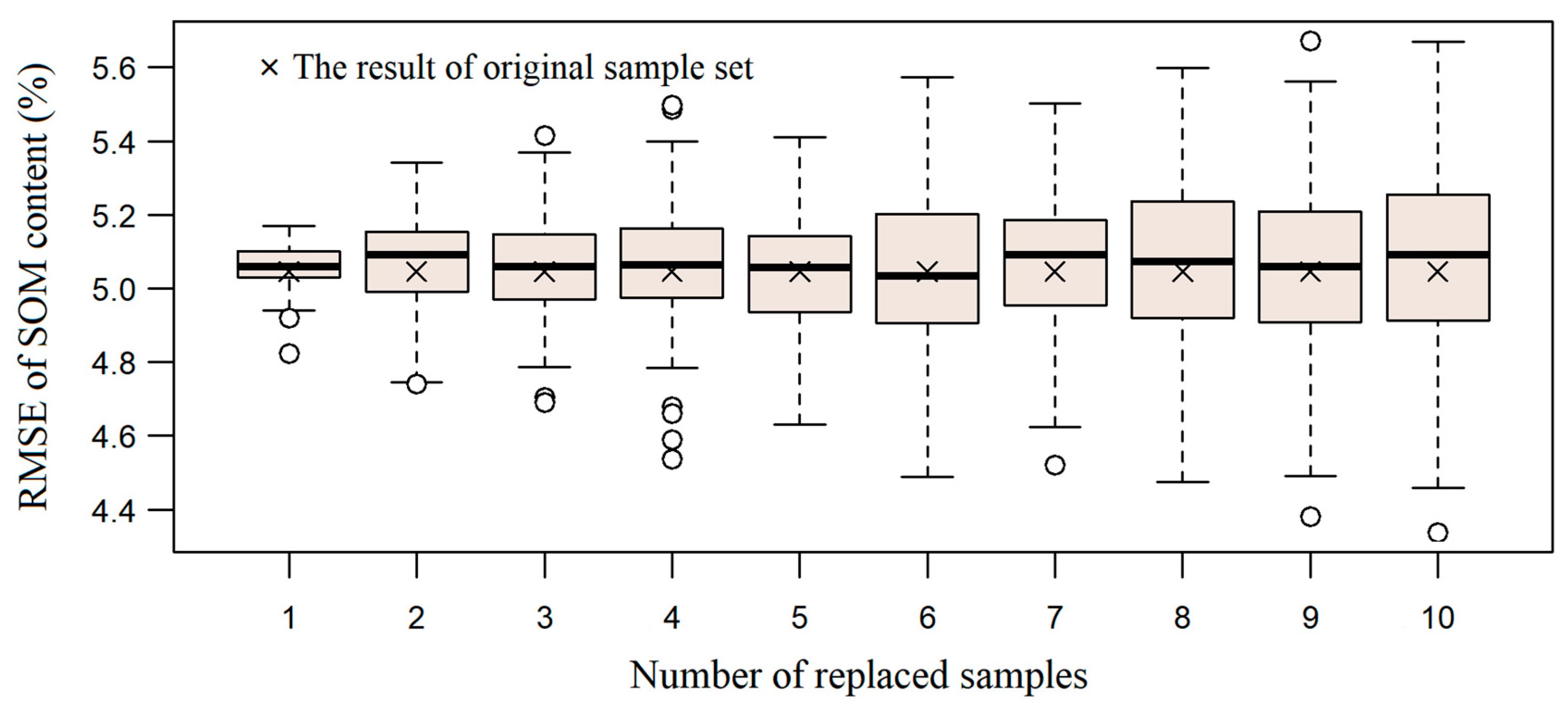
5.3. Substitute Samples for Stratified Random Sampling
5.3.1. Sample Layout
5.3.2. The Effect on Soil Mapping
5.4. Further Discussion
6. Conclusions
Author Contributions
Funding
Acknowledgments
Conflicts of Interest
References
- McBratney, A.B.; Mendonça Santos, M.L.; Minasny, B. On digital soil mapping. Geoderma 2003, 117, 3–52. [Google Scholar] [CrossRef]
- Brus, D.J. Improving design-based estimation of spatial means by soil map stratification. A case study of phosphate saturation. Geoderma 1994, 62, 233–246. [Google Scholar] [CrossRef]
- Brus, D.J.; Gruijter, J.J.D. Random sampling or geostatistical modelling? Choosing between design-based and model-based sampling strategies for soil (with discussion). Geoderma 1997, 80, 1–44. [Google Scholar] [CrossRef]
- Zhu, A.X.; Yang, L.; Li, B.L.; Qin, C.Z.; English, E.; Burt, J.E.; Zhou, C.H. Purposive sampling for digital soil mapping for areas with limited data. In Digital Soil Mapping with Limited Data; Hartemink, A.E., McBratney, A.B., Mendonca Santos, M.L., Eds.; Springer: New York, NY, USA, 2008; pp. 233–245. [Google Scholar]
- Yang, L.; Zhu, A.X.; Qi, F.; Qin, C.Z.; Li, B.L.; Pei, T. An integrative hierarchical stepwise sampling strategy and its application in digital soil mapping. Int. J. Geogr. Inf. Sci. 2013, 27, 1–23. [Google Scholar] [CrossRef]
- Long, J.; Liu, Y.; Xing, S.; Qiu, L.; Huang, Q.; Zhou, B.; Shen, J.; Zhang, L. Effects of sampling density on interpolation accuracy for farmland soil organic matter concentration in a large region of complex topography. Ecol. Indic. 2018, 93, 562–571. [Google Scholar] [CrossRef]
- Zeraatpisheh, M.; Ayoubi, S.; Jafari, A.; Finke, P. Comparing the efficiency of digital and conventional soil mapping to predict soil types in a semi-arid region in Iran. Geomorphology 2017, 285, 186–204. [Google Scholar] [CrossRef]
- Zhang, S.J.; Zhu, A.X.; Liu, J.; Yang, L.; Qin, C.Z.; An, Y.M. An heuristic uncertainty directed field sampling design for digital soil mapping. Geoderma 2016, 267, 123–136. [Google Scholar] [CrossRef] [Green Version]
- Roudier, P.; Hewitt, A.E.; Beaudette, D.E. A conditioned Latin hypercube sampling algorithm incorporating operational constraints. In Digital Soil Assessments and Beyond; Minasny, B., Malone, B.P., McBratney, A.B., Eds.; CRC Press: Boca Raton, FL, USA, 2012; pp. 227–231. [Google Scholar]
- Mulder, V.L.; De Bruin, S.; Schaepman, M.E. Representing major soil variability at regional scale by constrained Latin Hypercube Sampling of remote sensing data. Int. J. Appl. Earth Obs. 2013, 21, 301–310. [Google Scholar] [CrossRef]
- Clifford, D.; Payne, J.E.; Pringle, M.J.; Searle, R.; Butler, N. Pragmatic soil survey design using flexible Latin hypercube sampling. Comput. Geosci. 2014, 67, 62–68. [Google Scholar] [CrossRef]
- Kidd, D.; Malone, B.; Mcbratney, A.; Minasny, B.; Webb, M. Operational sampling challenges to digital soil mapping in Tasmania, Australia. Geoderma Regional 2015, 4, 1–10. [Google Scholar] [CrossRef]
- Wei, T.F. The Research of Calculating Alternative Samples of Soil Samples in Mobile Environment. Master’s Thesis, Nanjing Normal University, Nanjing, China, 2017. (In Chinese with English Abstract). [Google Scholar]
- Zhu, A.X.; Yang, L.; Li, B.L.; Qin, C.Z.; Pei, T.; Liu, B.Y. Construction of membership functions for predictive soil mapping under fuzzy logic. Geoderma 2010, 155, 164–174. [Google Scholar] [CrossRef] [Green Version]
- Zhu, A.X.; Band, L.; Vertessy, R.; Dutton, B. Derivation of soil properties using a soil land inference model (SoLIM). Soil Sci. Soc. Am. J. 1997, 61, 523–533. [Google Scholar] [CrossRef]
- Zhu, A.X.; Lu, G.N.; Liu, J.; Qin, C.Z.; Zhou, C.H. Spatial prediction based on Third Law of Geography. Ann. GIS 2018, 24, 225–240. [Google Scholar] [CrossRef]
- Zhu, A.X.; Liu, J.; Du, F.; Zhang, S.J.; Qin, C.Z.; Burt, J.; Behrens, T.; Scholten, T. Predictive soil mapping with limited sample data. Eur. J. Soil Sci. 2015, 66, 535–547. [Google Scholar] [CrossRef] [Green Version]
- Stevens, S.S. On the theory of scales of measurement. Science 1946, 103, 677–680. [Google Scholar] [CrossRef] [PubMed]
- Zhu, A.X.; Band, L. A knowledge-based approach to data integration for soil mapping. Can. J. Remote Sens. 1994, 20, 408–418. [Google Scholar] [CrossRef]
- Chen, Z.Q.; Chen, Z.B.; Chen, H.B.; Chen, L.H. Spatial relationship between soil fertility quality and human activities accessibility in the red eroded area of southern China: A case study in Zhuxi Watershed, Changting County, Fujian Province. Sci. Soil Water Conserv. 2012, 10, 103–107, (In Chinese with English Abstract). [Google Scholar]
- Cost Distance—Help | ArcGIS Desktop. Available online: http://pro.arcgis.com/en/pro-app/tool-reference/spatial-analyst/cost-distance.htm (accessed on 17 July 2018).
- Yang, L.; Zhu, A.X.; Zhao, Y.G.; Li, D.C.; Zhang, G.L.; Zhang, S.J.; Band, L.E. Regional Soil Mapping Using Multi-Grade Representative Sampling and a Fuzzy Membership-Based Mapping Approach. Pedosphere 2017, 27, 344–357. [Google Scholar] [CrossRef]
- Qin, C.Z.; Zhu, A.X.; Pei, T.; Li, B.L.; Scholten, T.; Behrens, T.; Zhou, C.H. An approach to computing topographic wetness index based on maximum downslope gradient. Precis. Agric. 2011, 12, 32–43. [Google Scholar] [CrossRef]
- Zhang, S.J.; Zhu, A.X.; Liu, W.L.; Liu, J.; Yang, L. Mapping detailed soil property using small scale soil type maps and sparse typical samples. Chin. Geogr. Sci. 2013, 23, 680–691. [Google Scholar] [CrossRef]
- Zeng, C.Y.; Yang, L.; Zhu, A.X.; Rossiter, D.G.; Liu, J.; Liu, J.Z.; Qin, C.Z.; Wang, D.S. Mapping soil organic matter concentration at different scales using a mixed geographically weighted regression method. Geoderma 2016, 281, 69–82. [Google Scholar] [CrossRef] [Green Version]
- Yu, K.Z.; Duan, T.W.; Li, D.H.; Peng, J.F. Landscape accessibility as a measurement of urban green system. City Plan. Rev. 1999, 8, 8–11, (In Chinese with English Abstract). [Google Scholar]
- Brus, D.J.; Noij, I.G.A.M. Designing sampling schemes for effect monitoring nutrient leaching from agricultural soils. Eur. J. Soil Sci. 2008, 59, 292–303. [Google Scholar] [CrossRef]
- Hammersley, J.M.; Handscomb, D.C. Monte Carlo Methods; Chapman and Hall: London, UK, 1979. [Google Scholar]
- Lesch, S.M.; Strauss, D.J.; Rhoades, J.D. Spatial prediction of soil salinity using electromagnetic induction techniques: II. An efficient spatial sampling algorithm suitable for multiple linear-regression model identification and estimation. Water Resour. Res. 1995, 31, 387–398. [Google Scholar] [CrossRef]
- Razakamanarivo, R.H.; Grinand, C. Mapping organic carbon stocks in eucalyptus plantations of the central highlands of Madagascar: A multiple regression approach. Geoderma 2011, 162, 335–346. [Google Scholar] [CrossRef]
- Aurenhammer, F. Voronoi Diagrams—A survey of a fundamental geometric data structure. ACM Comput. Surv. 1991, 23, 345–405. [Google Scholar] [CrossRef]
- Duyckaerts, C.; Godefroy, G. Voronoi tessellation to study the numerical density and the spatial distribution of neurones. J. Chem. Neuroanat. 2000, 20, 83–92. [Google Scholar] [CrossRef]


| Slope (°) | Cost Value |
|---|---|
| 0–5 | 1 |
| 5–10 | 3 |
| 10–20 | 5 |
| 20–30 | 7 |
| 30–35 | 9 |
| Land-Use Type | Cost Value |
|---|---|
| Urban land, rural resident land, other construction land | 1 |
| Bare soil | 2 |
| Bare rock and gravel, low coverage grassland | 3 |
| High coverage grassland, dry land, sparse woodland, other woodland | 5 |
| Paddy field | 6 |
| Dense woodland, beach | 7 |
| bushland | 9 |
| Lakes, river channels, reservoirs and pits | +∞ |
| Inaccessible Sample | Sampling Strategy | Substitute Location | Sampling Scenario | Substitutive Score | Accessibility Score |
|---|---|---|---|---|---|
| Stratified random sampling | Instant sampling | 1.0 | 0.93 | ||
| Subsequent sampling | 1.0 | 0.99 | |||
| purposive sampling | Instant sampling | 0.92 | 0.64 | ||
| Subsequent sampling | 0.92 | 0.99 |
| Number of Inaccessible Samples | The Percentage of Successfully Predicted Area to Study Area | ||
|---|---|---|---|
| Threshold = 0.4 | Threshold = 0.3 | Threshold = 0.2 | |
| 0 | 98.67 % | 96.20 % | 86.13 % |
| 1 | 98.66 % | 96.19 % | 86.12 % |
| 2 | 98.64 % | 96.15 % | 86.09 % |
| 3 | 98.62 % | 96.14 % | 86.07 % |
| 4 | 98.62 % | 96.13 % | 86.07 % |
| 5 | 98.62 % | 96.13 % | 86.07 % |
| 6 | 98.57 % | 96.04 % | 86.02 % |
| 7 | 98.52 % | 95.95 % | 85.92 % |
| 8 | 98.54 % | 95.99 % | 85.96 % |
| 9 | 98.53 % | 95.99 % | 85.99 % |
| 10 | 98.49 % | 95.91 % | 85.87 % |
© 2019 by the authors. Licensee MDPI, Basel, Switzerland. This article is an open access article distributed under the terms and conditions of the Creative Commons Attribution (CC BY) license (http://creativecommons.org/licenses/by/4.0/).
Share and Cite
Zhao, F.-H.; Qin, C.-Z.; Wei, T.-F.; Ma, T.-W.; Qi, F.; Liu, J.-Z.; Zhu, A.-X. Dynamic Recommendation of Substitute Locations for Inaccessible Soil Samples during Field Sampling Campaign. ISPRS Int. J. Geo-Inf. 2019, 8, 127. https://doi.org/10.3390/ijgi8030127
Zhao F-H, Qin C-Z, Wei T-F, Ma T-W, Qi F, Liu J-Z, Zhu A-X. Dynamic Recommendation of Substitute Locations for Inaccessible Soil Samples during Field Sampling Campaign. ISPRS International Journal of Geo-Information. 2019; 8(3):127. https://doi.org/10.3390/ijgi8030127
Chicago/Turabian StyleZhao, Fang-He, Cheng-Zhi Qin, Teng-Fei Wei, Tian-Wu Ma, Feng Qi, Jun-Zhi Liu, and A-Xing Zhu. 2019. "Dynamic Recommendation of Substitute Locations for Inaccessible Soil Samples during Field Sampling Campaign" ISPRS International Journal of Geo-Information 8, no. 3: 127. https://doi.org/10.3390/ijgi8030127