Integration, Processing and Dissemination of LiDAR Data in a 3D Web-GIS


Department of Geoinformatics, Faculty of Electronics, Telecommunication and Informatics, Gdansk University of Technology, 80-233 Gdansk, Poland
*
Author to whom correspondence should be addressed.
ISPRS Int. J. Geo-Inf. 2019, 8(3), 144; https://doi.org/10.3390/ijgi8030144
Submission received: 5 February 2019
/
Revised: 11 March 2019
/
Accepted: 15 March 2019
/
Published: 19 March 2019
(This article belongs to the Special Issue Multidimensional and Multiscale GIS)
Abstract
:The rapid increase in applications of Light Detection and Ranging (LiDAR) scanners, followed by the development of various methods that are dedicated for survey data processing, visualization, and dissemination constituted the need of new open standards for storage and online distribution of collected three-dimensional data. However, over a decade of research in the area has resulted in a number of incompatible solutions that offer their own ways of disseminating results of LiDAR surveys (be it point clouds or reconstructed three-dimensional (3D) models) over the web. The article presents a unified system for remote processing, storage, visualization, and dissemination of 3D LiDAR survey data, including 3D model reconstruction. It is built with the use of open source technologies and employs open standards, such as 3D Tiles, LASer (LAS), and Object (OBJ) for data distribution. The system has been deployed for automatic organization, processing, and dissemination of LiDAR surveys that were performed in the city of Gdansk. The performance of the system has been measured using a selection of LiDAR datasets of various sizes. The system has shown to considerably simplify the process of data organization and integration, while also delivering tools for easy discovery, inspection, and acquisition of desired datasets.
1. Introduction
In recent years, the proliferation of affordable Light Detection and Ranging (LiDAR) scanners has caused a rapid increase in their application. In contrast to expensive models, low-cost scanners are characterized with an effective scan range of under 10 m, which means that they are often used to collect information regarding single objects (e.g., buildings, monuments, etc.) at a time. This, in turn, results in a growing number of medium-volume point-based datasets that need to be categorized and classified before further processing. Moreover, LiDAR data is usually archived in binary files in the LASer (LAS) format, which is an open standard of three-dimensional (3D) data storage [1]. The format, although efficient for the storage of, for example, colour and classification information, is not particularly convenient for data management and dissemination. As the LAS standard does not allow for data cross-referencing, users must devise their own methods of organizing LiDAR datasets. Whereas, measurements that are performed on a large scale are easily placed in the context of a geographic grid, small-scale surveys that are performed in close proximity to one another are much harder to organize. Moreover, because the binary LAS format can only be effectively and reliably parsed using specialized desktop software, the online sharing of LiDAR datasets is even more complex.
This situation is particularly problematic for researchers, who are often interested in the point clouds of a particular quality. If data is stored in binary LAS files, then end users have no means to inspect it before downloading, which may result in the unnecessary loss of time and bandwidth. In consequence, new methods of online processing and the visualization of LiDAR data have been an active area of research for many years. In 2011, Krishnan et al. [2] presented web architecture for community access to LiDAR data, while Kuder and Zalik [3] proposed a method of serving subsets of LiDAR data in their original format via a Representational State Transfer (REST) service. In 2012, Lewis et al. [4] proposed a framework for LiDAR data storage, segmentation, and web-based streaming. Over the following years, Mao and Cao [5] proposed a method of remote 3D visualization of LiDAR data using HyperText Markup Language version 5 (HTML5) technologies, Maravelakis et al. [6] presented the Web-based point-cloud viewer utilising the Three.js Web Graphics Library (WebGL) Abstraction Layer, Nale [7] designed a framework for processing, querying, and web-based streaming of LiDAR data, Li et al. [8] proposed a framework for online LiDAR data processing that is based on Apache Hadoop, while von Schwerin et al. [9] presented a system for 3D visualization of pre-processed LiDAR data using WebGL. More recently, Schmiemann et al. [10] proposed a method for online mapping of data directly obtained form Unmanned Aerial Vehicles (UAV’s), Huang and Wang proposed a system for online processing and the visualization of LiDAR point clouds using WebGL [11], while Bohak et al. [12] presented a framework for online 3D visualization of LiDAR data while using Three.js and Potree.
Although the proposed solutions are very diverse in nature, all of them must deal with the main problem stemming from the use of web solutions. Namely, the successful processing and dissemination of LiDAR data in the web environment requires the source LAS files to be converted into a format which is better suited for online applications. Moreover, the evident lack of industry standards means that the exchange of such data between two different web-based applications is not possible without the prior modification of one of them to adopt the other’s method of data distribution. None of the existing solutions addresses this issue on the conceptual level. What is more, although the functionality that is offered by web solutions based on remote access to LiDAR measurement data is constantly expanding (e.g., the tools that are offered by GeoSignum allow not only for efficient access to large LiDAR data resources, but also provide advanced functions that include feature extraction, automatic object classification, statistical and spatial analysis tools, among others [13]), the users are forced to rely on the closed, commercial software on which they have no influence, which further limits the interoperability.
In the case of two-dimensional (2D) raster and vector data, the issue of data exchange between different systems has been solved with the adoption of open standards, such as Web Map Service (WMS) [14] and Web Feature Service (WFS) [15], which have been established by the Open Geospatial Consortium (OGC). While a standard format of storing 3D data exists in the form of the OGC CityGML [16], it has been primarily designed for representing buildings, roads, vegetation, terrain topography, and other elements of a three-dimensional city. In consequence, it does not provide efficient methods of data streaming and visualization (such as tiling of larger datasets), which means that the user needs to solve these important problems [17]. The Indexed 3D Scene Layer (I3S) format, defined by the Environmental Systems Research Institute (ESRI), handles issues such as 3D data tiling, compression, and level-of-detail. However, at the time of writing, the standard has only been adopted by commercial software, which considerably limits its application [18].
This being said, the recent years have witnessed the advent of a new open standard for unified storage and online dissemination of various types of three-dimensional data, including point sets and 3D models. The authors of the popular Cesium library have proposed the standard, named 3D Tiles, which is an open source library for the 3D visualization of geospatial data [19]. As such, Cesium provides excellent support for the online visualization of geographic information in the 3D Tiles format, which enables the construction of open source Web-based Geographic Information System (Web-GIS) applications for the dissemination of large-volume 3D data [20]. Recently, version 1.0 of the 3D Tiles specification has entered the process to become an OGC Community Standard [21]. In consequence, the combination of Cesium and 3D Tiles constitutes an appealing open source solution for 3D data dissemination. The advantages of utilizing these technologies include not only the convenient manner of data sharing and exchange, but also the easy handling of “the level of detail”, owing to the hierarchical organization of 3D Tiles.
Another important issue that is related to LiDAR data storage, processing, visualization, and dissemination is the geometric model that is used for its representation. The initial form of LiDAR data, as represented by an unorganized 3D point cloud, has many disadvantages, including poor support of representing objects and their attributes, low efficiency with respect to used processing power and memory resources (as even primitive surfaces, such as flat building roofs, are represented by dense groups of points), and low visualization quality. As a result, certain areas of research prefer the use of simpler procedurally generated models [22]. For these reasons, a different type of geometric model represents 3D spatial data, which relies on expressing three-dimensional objects in the form of surfaces consisting of higher order geometric structures, known as triangulated irregular network (TIN) models. As the overall shape of many real-world objects usually contains some semi-flat surfaces, representing them in the form of solid meshes results in improvements to storage space, bandwidth consumption, use of central processing unit (CPU), and memory resources as well as visualization quality. As a result, the methods of automatic shape recovery and the construction of more composed geometric models of spatial objects from point cloud data are crucial with respect to many applications of LiDAR measurements, and they have been the subject of extensive research for over a decade [23]. In consequence, several methods exist and different approaches are applied, depending on the type of scanned objects and application specifics; however, attempts to create a more universal approach to the problem are also carried out [24,25]. Thus, it may be expected that, in the near future, tools for shape recovery and higher order geometric model construction should become a standard element of systems that are dedicated to the management and dissemination of LiDAR point cloud data.
In the above context, the article presents a unified system for remote processing, storage, visualization, and dissemination of 3D objects that are obtained from LiDAR surveys. The system is built with the use of open source technologies and it employs the 3D Tiles standard for data dissemination. Those design choices address several problems that were identified within the previously discussed solutions. In particular, when compared to the present state-of-the-art, the proposed system offers functionality that combines and exceeds the capabilities of individual existing systems, including:
- upload, integration and sharing of data provided by different users;
- automatic 3D TIN model construction from point clouds for representation of spatial objects;
- storage and dissemination of data with the use of community standard open formats and protocols; and,
- online 3D visualization of original point clouds as well as reconstructed 3D models.
Section 2 presents the detailed architecture of the developed system of the article, which also explains the functionalities of its modules. Section 3 exemplifies the application of the system to LiDAR data processing and dissemination. Section 4 discusses the performance of the system when processing datasets of different sizes. Finally, Section 5 summarizes the presented work and outlines potential future research and development.
2. The Proposed System
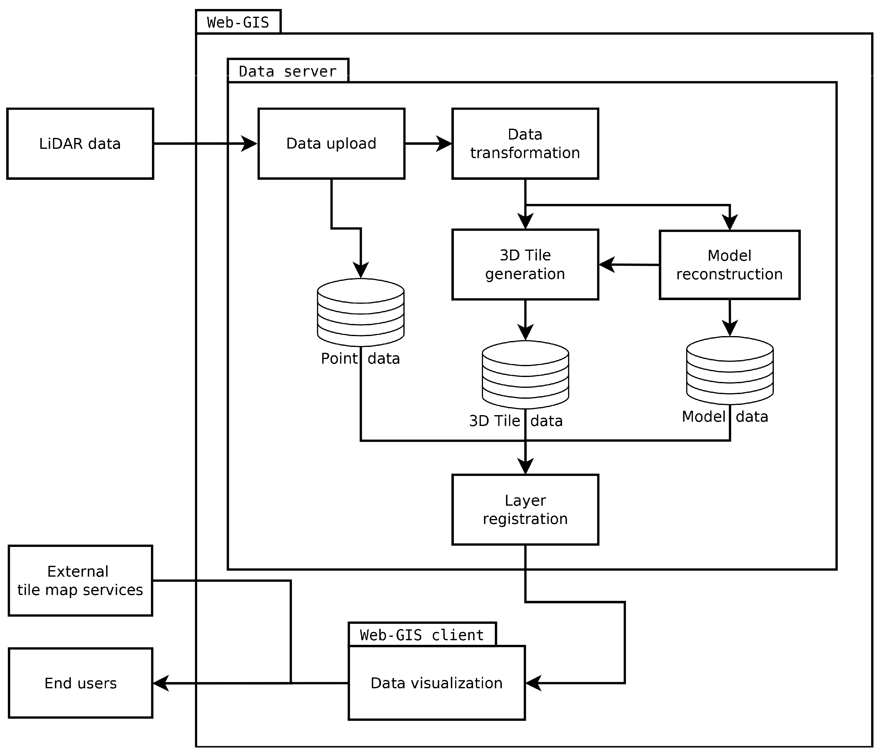
The presented system has been designed with the purpose of online processing, storage, visualization, and dissemination of 3D objects that were obtained from LiDAR surveys. Figure 1 presents the architecture of the system.
The results of LiDAR surveys are remotely uploaded to the Data server via the system’s Data upload module. There, the user needs to input some basic information regarding the data, such as its name and category. Once the upload is complete, the data is passed on to the data transformation module. There, the data is parsed and pre-processed. Afterwards, the results are passed on to the 3D Tile generation module, as well as Model reconstruction module. The former uses the pre-processed point data to construct 3D Tiles of the scanned object, while the latter attempts to reconstruct the object in the form of a three-dimensional model. The products of those two modules are then registered in their respective databases. The addresses of both 3D Tile and model versions of the scanned object are then passed on to the Layer registration module, which is responsible for generating a categorized list of all layers in the system for use with the Web-GIS client module. The client module provides a multidimensional visualization of data stored within the system with the option of overlaying it on data obtained from external mapping services. The client also enables instant switching between point and 3D representation of every object and it permits an on-demand download of source point data.
The following subsections list the technology and implementation specifics of each module.
2.1. Data Upload
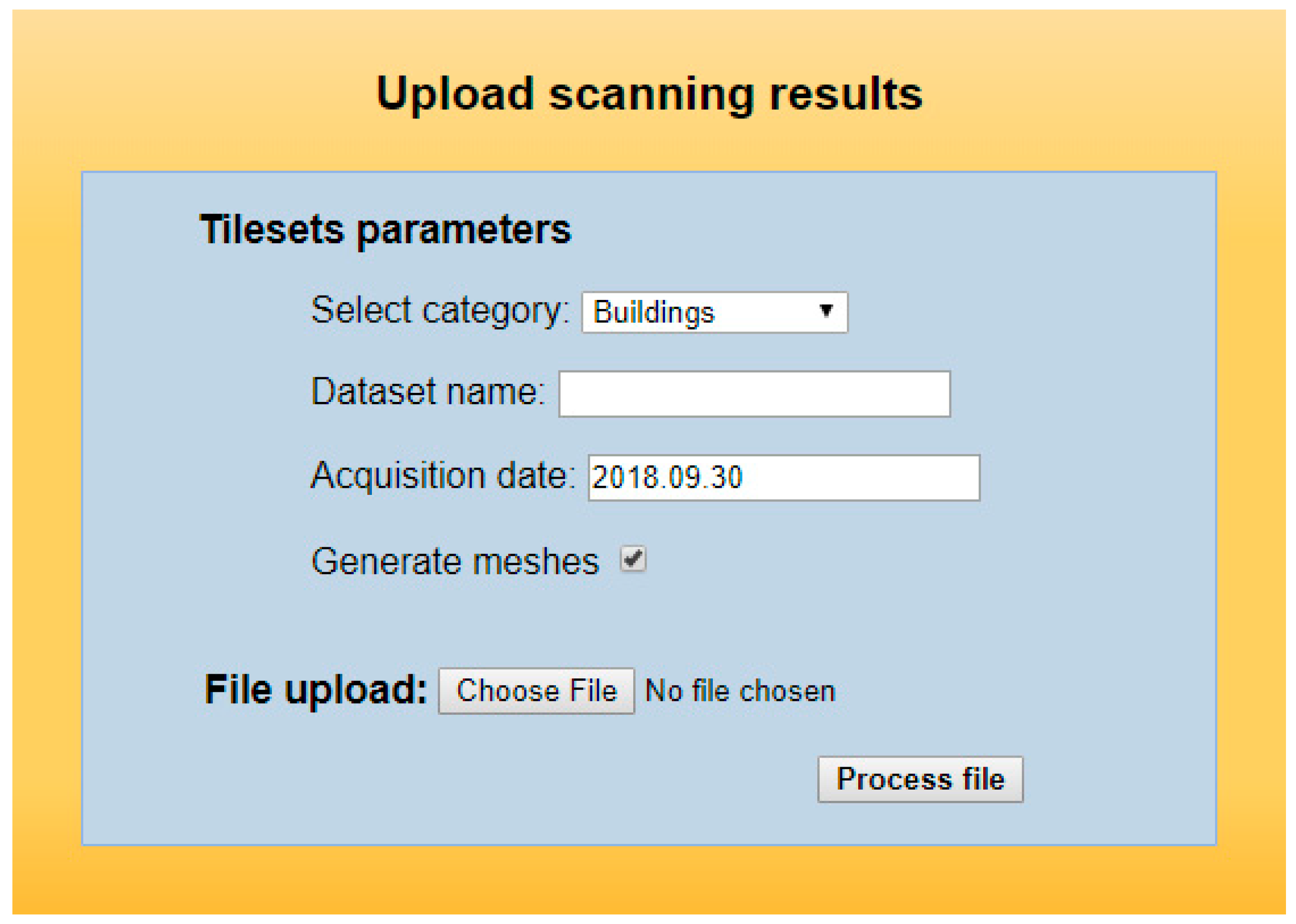
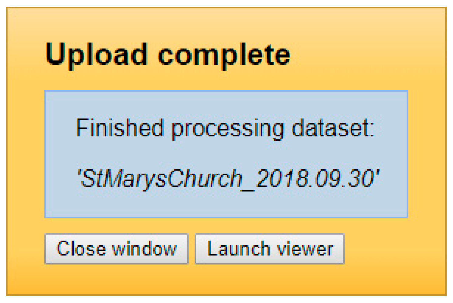
The results of LiDAR surveys are delivered to the system through a dedicated data upload module. The module exposes a straightforward frontend, which consists of a website that enables the user to select a local file to be transferred to the server. Alongside the location of the file, the user must specify several parameters, including the name of the uploaded dataset, its category (building, monument, terrain object, etc.), and date of acquisition. Once the values of all the required attributes have been provided, the user may proceed with uploading the file to the server. The upload process is asynchronously realized, which enables the user to be notified of transfer progress. Once data upload is complete, the file is automatically processed, and the user is notified of the progress and results. If the server encountered no errors, then the user is notified that the processing results may be viewed while using the Web-GIS client. The uploaded file is stored in the server database, from where it may be accessed by the Data transformation module, as well as being downloaded directly by end users.
2.2. Data Transformation
Once the LiDAR data has been uploaded, the Data transformation module automatically processes it. Data processing starts with decompression. Subsequently, the data is parsed. As the surface scanning results of a researched object are stored in the form of a point cloud in the European Petroleum Survey Group coordinate system no. 2180 (EPSG:2180) (which is unique for the entire area of Poland), the uploaded data is transformed to the Earth-Centered, Earth-Fixed (ECEF) coordinate system and then divided into a regular tile grid. In order to enable high-precision rendering of the converted dataset (which prevents display artifacts, such as jittering), all of the point positions are stored as values relative to the calculated center position of their associated tile. Finally, the point cloud data for each tile is converted to binary PNTS format to make it compatible with 3D Tiles Point Clouds. This dataset is then passed on to the 3D Tile generation module, while the original LAS file is passed on to the Model reconstruction module.
2.3. D Tile Generation
The 3D Tiles standard allows for the seamless integration of 3D data obtained from various sources in a hierarchical tree-like structure. The structure covers the entire surface of the Earth in tiles of various sizes and shapes. The tile shapes are defined by their bounding volumes (consisting of minimum and maximum longitude, latitude, and height relative to the World Geodetic System 1984 <WGS84> ellipsoid), which completely enclose their contents. Each tile may contain child tiles, which in turn may contain various types of 3D data as well as other child tiles, provided that the parent’s bounding volume contains all of the data stored within the child tiles. Currently, the 3D Tiles standard supports several different types of tiles. These consist of [19]:
- Point Cloud tiles, which contain arrays of 3D points;
- Batched 3D Model tiles, which contain solid 3D shapes based on the GL Transmission Format (glTF);
- Instanced 3D Model tiles, which contain many instances of a single model; and,
- Composite tiles, which may contain a combination of all the above.
Moreover, the standard defines several ways in which a 3D Tile may be divided into subtiles. These include k-d tree subdivision (where each tile has two children separated by a splitting plane parallel to the x, y, or z axis), the quadtree subdivision (where each tile is divided into four uniform children in 2D, i.e., the division is done with respect to the horizontal plane), the octree subdivision (similar to quadtree, but with division into eight children in 3D, i.e., by splitting a tile into two parts along each axis x, y, and z), and a grid subdivision (which allows for the definition of uniform, non-uniform, as well as overlapping grids for an arbitrary number of child tiles). Due to the presented system being designed to store data obtained from surveys that were made in various locations and on a varied scale, the results are uniformly divided in space and stored in the context of a regular grid with a tile size of 20 × 20 m (400 m2). Previous research has shown that, for dense point clouds, this tile size enables the coverage of a relatively large area with a single tile, while ensuring that its physical size is small enough to be easily transferred over the web [20]. Every processed dataset is subdivided into appropriate sections of the grid, with every section being defined by its own JSON-based tile set definition file. The results are placed in the appropriate subfolder of the 3D Tile database, from where they may be accessed by any application that is compatible with the standard.
2.4. Model Reconstruction
Aside from storage and visualization, the primary function of the presented system is the processing of collected data for the purpose of model reconstruction. In this context, the LiDAR data that was collected within the system is passed through the Model reconstruction module, where it undergoes several stages of processing. The first step of model reconstruction involves data regularization. At this point, the original point cloud is simplified and then placed within the context of a grid with a fixed resolution. The second step involves denoising the regularized data. After the data has been regularized and denoised, the contents of the point cloud are classified into several categories, including ground, objects (e.g., buildings), and greenery. The classification algorithm first attempts to detect large terrestrial objects and assign them to a new class, in order to separate them from ground points (using an approach that is similar to the one applied to underwater objects in [24]). The class assignment of each detected object is then corrected based on the object’s colour data. Afterwards, the Poisson Surface Reconstruction algorithm [26] is performed for selected objects with the use of MeshLab [27] to generate solid 3D meshes. If the original point cloud contains information regarding colours, this data is used to interpolate a texture for the reconstructed 3D objects. The textured 3D models are then saved in the open Wavefront Object (OBJ) format [28], after which they are compressed using the open ZIP archive format and then stored in the appropriate directory of the Model database. From there, the models may be downloaded and displayed in any application compatible with the standard. Finally, the reconstructed meshes are converted to binary B3DM format, which enables their dissemination as a part of Batched 3D Model tiles.
2.5. Layer Registration
Once the 3D Tiles containing processed LiDAR point cloud data, as well as reconstructed buildings (in OBJ format), have been stored in their respective databases, they need to be made available through the Web-GIS client. The client is built in Dynamic HyperText Markup Language (DHTML) technology, and thus the list of available layers is stored in a text file that contains javascript code, where the layers are grouped by their data type, origin, and categories. This code is imported by the client code, which causes it to be automatically parsed and interpreted when the client is initialized. In this context, the purpose of the Layer registration module is to generate an updated version of this layer file whenever a new dataset has been processed by the system.This functionality is provided by listing the contents of all data directories and storing the relative paths to tiles, 3D models, and original LAS files in the javascript file.
2.6. Data Visualization
The Web-GIS client was designed to provide online 3D visualization of reconstructed modes, as well as point clouds in the 3D Tiles format. The Cesium javascript library [29], which fulfills both of those requirements, was a natural choice for constructing the client. Cesium is an open source library for multidimensional data visualization, including the drawing of a 3D Earth based on the WGS84 ellipsoid with overlaid Digital Terrain Model data, as well as 3D objects that may change their state (e.g., position or animation frame) over time. Standard features that are supported by the library include drawing of the sun, stars, and Earth’s atmosphere, as well as dynamic lighting and shading (including self-shadows) of both terrain as well as overlaid objects. The latter may include raster data and vector features that may be integrated from multiple sources, such as WMS, Tile Map Service (TMS), Web Map Tile Service (WMTS), tile map services that are provided by OpenStreetMap (OSM), and Bing maps as well as 3D models in glTF and COLLADA formats, in addition to standard image files. All of the overlaid objects may be subject to custom animations, including the application of shaders (which include animated water and particle emitters) as well as changing their position and orientation according to the library’s internal time-of-day clock. Moreover, the library is very well optimized and it supports performance-enhancing techniques, such as level-of-detail, clipping, and culling, as well as a high precision Z-buffer for enhanced image quality. Using Cesium allows the client to provide 3D visualization of the Earth, which is represented by the WGS84 ellipsoid textured with satellite images. By default, the application uses the free Blue Marble dataset for texturing the planet. However, it is also possible to use external WMS to apply high-resolution Sentinel-2 imagery that were obtained from the free service that is provided by EOX IT Services GmbH [30]. Data in the client is organized in layers, a list of which is presented in a categorized manner in the application’s table of contents. The list presents a set of expandable nodes that correspond to data that is uploaded by the user. Each node contains information about the scanned object in the form of sets of 3D Tiles that contain either point clouds or 3D meshes (if their creation was requested during upload). By selecting proper nodes, the user has the option to either load or unload the specified tileset or download the corresponding data, such as the original point cloud or the 3D mesh file. The models and point clouds may be inspected in 3D context while using standard Cesium tools for zooming and panning the camera.
3. Application of the System to LiDAR Data Processing and Dissemination
The Department of Geoinformatics, Faculty of Electronics, Telecommunications and Informatics of the Gdansk University of Technology has developed and implemented the system for the purpose of automatic organization of LiDAR surveys that were performed in the city of Gdansk. Datasets that were collected by airborne or terrestrial LiDAR systems are copied onto a PC or laptop and then uploaded to the presented system, as shown in Figure 2.
Once the files have been processed, the user is redirected to the Web-GIS client, as shown in Figure 3.
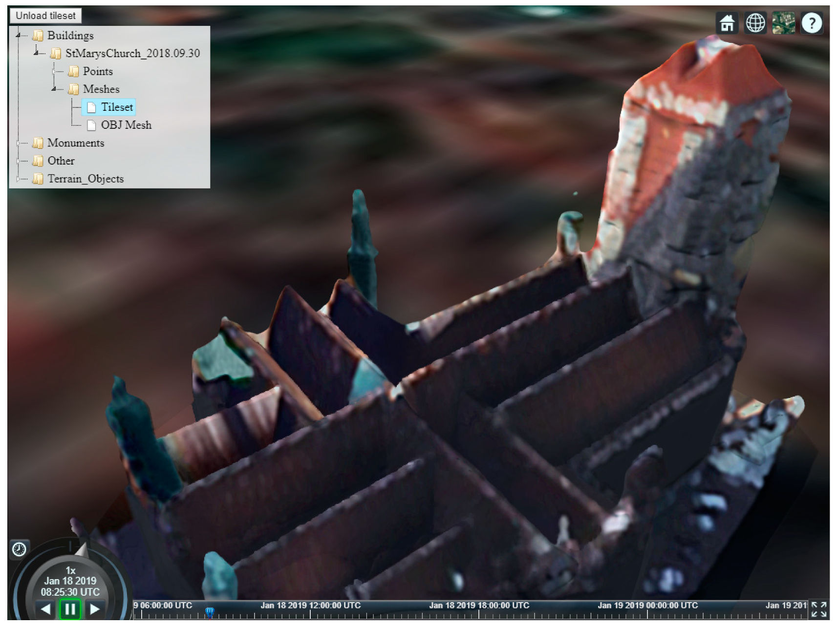
After clicking the Launch viewer button in the Data upload page, the user is transferred to the Web-GIS client module. By default, the client displays the most recently processed dataset in 3D model form. Other datasets may be selected from the client’s table of contents, as shown in the upper left corner of the Web-GIS interface. The datasets are categorized into “Buildings”, “Monuments”, “Terrain Objects”, and “Other”. Every category contains a list of datasets. The individual datasets contain “Points” and “Meshes” (if the user selected mesh generation during data upload). The former contains a reference to the point cloud in the 3D tiles format, as well as a link to download the original LAS file. The latter contains a reference to the reconstructed model in the 3D tiles format, as well as a link to download it in the OBJ format.
Clicking on an item in the table of contents activates the Load tileset button in the upper left corner of the screen. Clicking the button causes the Web-GIS client to download the selected dataset and display it by centering the camera on it. The Cesium library provides other available tools. They include a set of buttons in the upper right corner and a time control bar in the lower part of the screen. In the order of left to right, the buttons that enable centering the current view on the Gdansk University of Technology Faculty of Electronics, Telecommunications, and Informatics, changing the map view between 3D, 2D, and Columbus, changing the base layer from Blue Marble to a Sentinel-2 image, and displaying help. The time control bar enables the users to change the speed of time flow, as well as to change the current date. This action appropriately adjusts the position of the sun, which changes the scene lighting as well as shading of 3D models.
Figure 4 presents a reconstructed 3D model of the Basilica of St. Mary in Gdansk, as seen in the Web-GIS client.
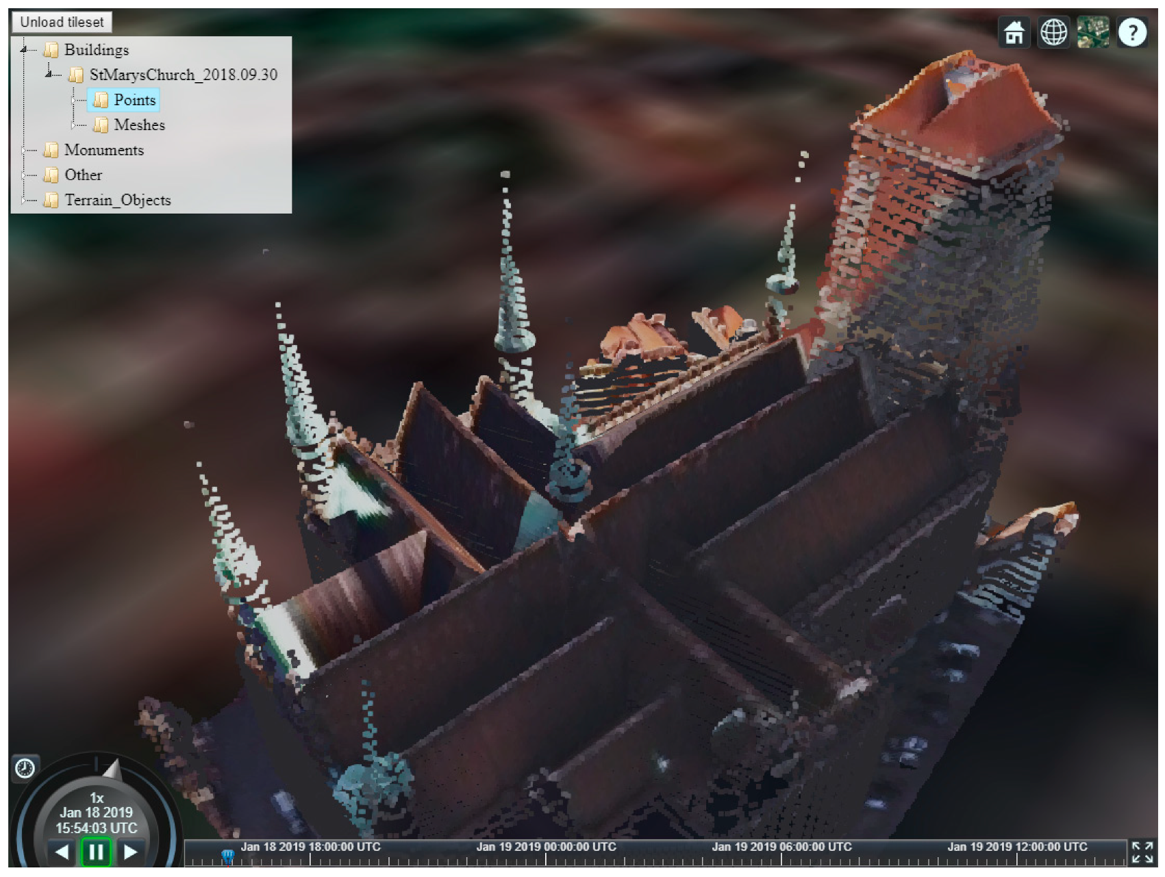
Clicking on other objects that are listed in the table of contents allows the user to load and display them in addition to the existing ones. For instance, selecting the “Points” category and selecting “Load tileset” shows the original point cloud dataset in addition to the 3D model. Selecting the “Meshes/tileset” option and clicking “Unload tileset” only leaves the 3D point cloud. Selecting “Meshes/OBJ Mesh” allows for downloading the 3D model directly to the user’s computer. Figure 5 presents the original point cloud of the Basilica of St. Mary in Gdansk, as seen in the Web-GIS client.
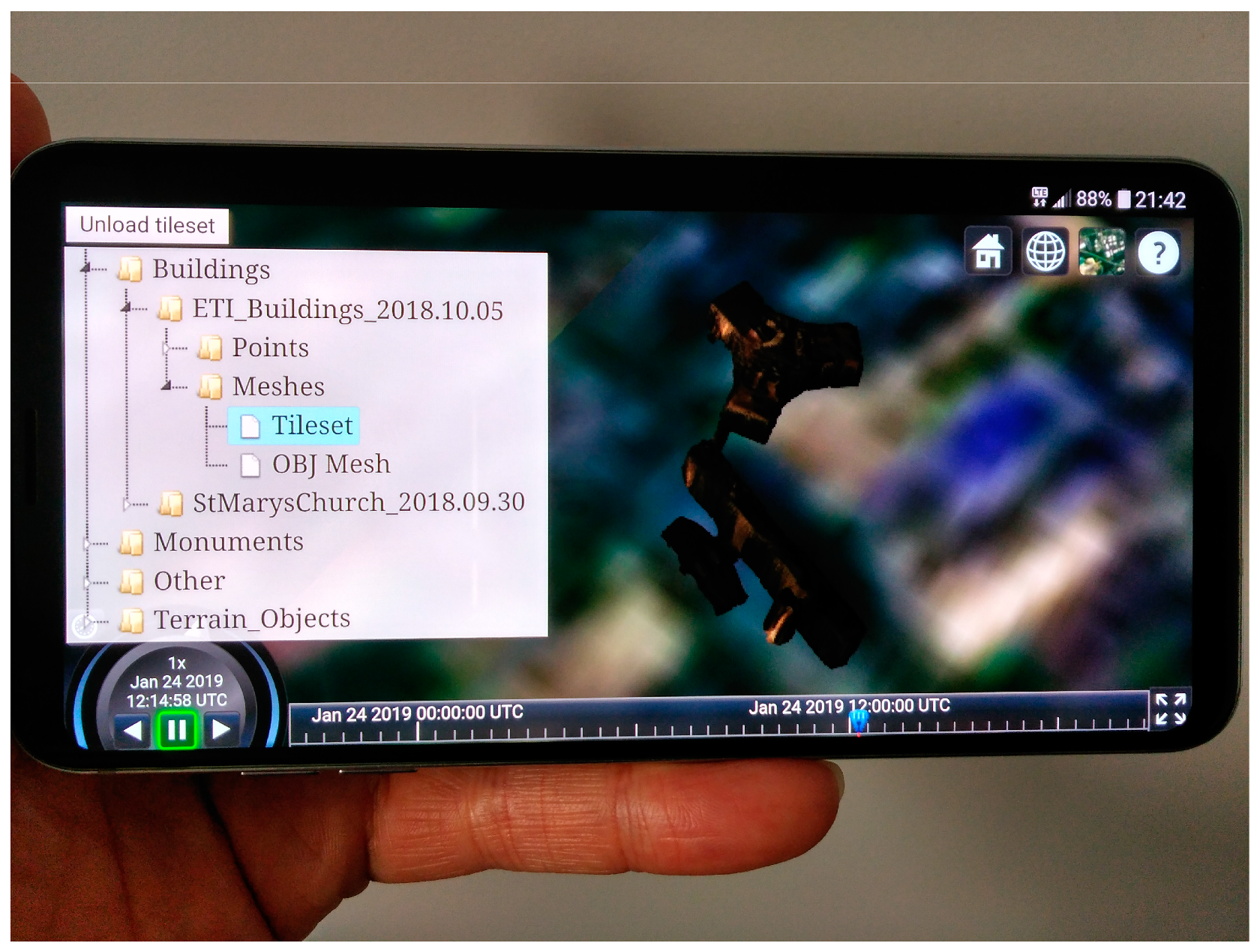
As the Web-GIS client has been strictly implemented with the use of HTML5 technologies, it can be run in any modern web browser, including mobile ones (provided that they support WebGL). Modern smartphones come equipped with fast Graphic Processing Units (GPU’s) and over 3 GB of RAM, which (in tandem with highly optimized rendering techniques that are offered by Cesium) enables the convenient use of the Web-GIS client on a mobile device. Figure 6 presents the Web-GIS client running on a smartphone that is equipped with a Snapdragon 835 chipset and 4 GB of RAM, displaying 3D meshes of the Gdansk University of Technology Faculty of Electronics, Telecommunications, and Informatics overlaid on a Sentinel-2 satellite image.
4. Discussion of System Performance
The system consists of two primary modules: the server, which is responsible for data storage and processing, and the client, which handles data 3D visualization. Thus, an analysis of the system’s performance should individually consider both of these elements.
4.1. Data Processing Performance
The server’s data processing performance has been measured while using LiDAR point clouds of various density and volume. As the algorithm performance was expected to scale with the size of input data, the number of vertices has been chosen as the principle for selecting point clouds for testing purposes. The input datasets included:
- Point cloud A: 249062 points
- Point cloud B: 158071 points
- Point cloud C: 72669 points
- Point cloud D: 15487 points
The tests have been performed on a server that is equipped with an Intel i7 8700K six-core (twelve-thread) CPU, 32 GB of RAM, and an eight-TB RAID-5 hard disk array. The tests measured the entire time of data processing, beginning with the uploaded file entering the Data transformation module, and ending with the Layer registration module updating the file containing the list of layers in the system. It should be noted that the CPU and disk configuration of the server permits certain operations in the system (e.g., model reconstruction and generation of Point Cloud 3D Tiles) to be performed in parallel. The measured characteristics included the processing time and RAM consumption. Table 1 presents the test results.
Table 1 presents the total processing time of a dataset from its admittance to the system to registration in the client layer list. During this time, several system modules, sometimes in parallel, process the datasets. In relation to the total processing time, the average processing times for individual system components are as follows:
- Data transformation: 8%
- Point Cloud tiles generation: 23%
- Batched 3D Model tiles generation: 92%, where 29% of total processing time is spent on data regularization, denoising and classification, 51% is spent on 3D surface reconstruction and building OBJ models and 12% is spent on converting the reconstructed mesh into B3DM format.
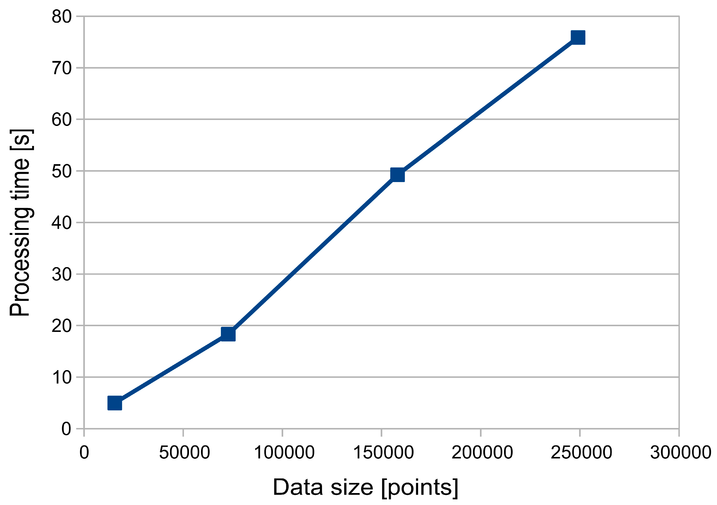
The time required for updating the client’s layer list was incomparably small (less than 1%), and thus it was omitted from the total. The recorded processing times for the used datasets are generally low and the same can be said about RAM consumption (in relation to the available system resources at least). The way that these characteristics will change for larger point clouds may be deduced by analyzing the evolution of those results in relation to the size of input data. Figure 7 presents the scaling of processing time in relation to the number of vertices in the processed point cloud.
As can be seen, the presented system provides linear scaling of processing time in relation to size of input data. While the certainly not as optimal as logarithmic, this type of performance scaling is preferred to the often-encountered polynomial one, where the processing time for larger datasets becomes disproportionally longer.
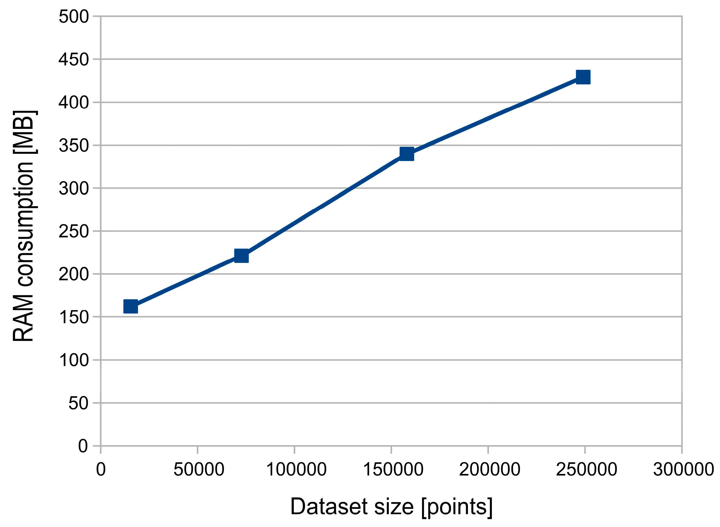
While processing a larger dataset will require more time, it will also need more RAM, which is a limited resource. Determining the maximum size of an input dataset that may be processed by the system in its current configuration requires an analysis of the scaling of RAM consumption in relation to input data size. Figure 8 presents the results of this analysis.
Similarly to processing time, the presented system provides linear scaling of RAM usage in relation to the size of input data. While RAM consumption could be further optimized, at the current rate, the server system should be able to process LiDAR clouds that consist of over 18 million points without the need to upgrade its operating memory.
4.2. Data Visualization Performance
The client’s data visualization performance has been measured by displaying the same LiDAR point cloud on several machines. Because, by default, Cesium does not redraw static scenes and only requests new video frames to be drawn when a change occurs, for the purpose of this test, a custom version of the client has been deployed with this optimization being disabled. This version of the client has then been executed on the following machines:
- Machine A: a Desktop-class PC equipped with an Intel Core i5 2500K quad core CPU, 16 GB of RAM and an Nvidia GeForce RTX 2080 Ti GPU.
- Machine B: a Laptop-class PC equipped with an Intel Core i7 3630QM quad core CPU with two hardware threads per core, 16 GB of RAM, and an Intel HD Graphics 4000 integrated GPU, in addition to a discrete Nvidia GeForce GTX 660M GPU.
- Machine C: a Smartphone that is equipped with a Snapdragon 835 System-on-Chip (SoC), which has two sets of cores (four “big” high-performance cores and four “little” high-efficiency cores) and 4 GB of RAM.
On every machine, the client performance has been measured when displaying the point cloud depicting the Basilica of St. Mary in Gdansk in the Google Chrome web browser, with a screen resolution of 1920 × 1080 pixels. In order to simulate real-world usage without inducing stutter that is caused by loading new assets, the displayed model was shifted to the left and right by several pixels while using the Client’s input controls. The measured performance characteristics included the number of video frames displayed per second (FPS), CPU use percentage, and RAM consumption. Table 2 presents the test results.
The obtained results show that running the Web-GIS client poses no problem for the Desktop-class PC. The system delivered an average of 60 frames per second, which is the maximum number that is allowed on a 60 Hz display without disabling synchronization. The application used 175 MB of RAM, which is a moderate amount when considering the available system resources (16 GB). Average CPU usage was around 15%, which corresponds to 60% usage of a single core out of the four that are available.
When considering the results that were obtained on the Laptop-class PC, the performance was substantially different, depending on the active hardware components. The system delivered an average of 15 frames per second when using the integrated Intel GPU, which are known for their low performance. However, running the application with the built-in discrete Nvidia GeForce 660M GPU delivered a stable performance level of about 55 frames per second. The application used around 176 MB of RAM, which is in line with the RAM consumption that was recorded on the Desktop-class PC. Average CPU usage was around 7%, which on a machine with eight logical cores corresponds to 60% usage of one of them.
The results that were obtained on the Smartphone are the most interesting. The system delivered an average of 25 frames per second, which not only provided good system responsiveness, but also exceeded the performance that was offered by the Intel integrated GPU on the Laptop. The application used around 298 MB of RAM, which is about 60% more than on other tested systems. This may be a result of using a different version of Google Chrome that specifically was built for the Android operating system. Still, the higher amount of consumed RAM is entirely acceptable when considering the available system resources (4 GB). Average CPU usage was around 28%, which corresponds to 100% usage of a single core and 12% use of a secondary core. However, it should be noted that the recorded usage corresponds to the four “little” cores, which are the low-performance, power-efficient part of the SoC. The usage of the four high-performance “big” cores was marginal (around 5%), which indicates that delivering a high level of performance when displaying LiDAR survey results on a mobile device does not require a sacrifice in power efficiency.
4.3. Performance limitations
Testing the system performance using datasets that were collected during real-world usage can deliver important metrics for establishment of data processing efficiency scaling. However, when discussing performance limitations, it is necessary to perform the tests using large volume data, which may not always be readily available. In order to test scenarios in which system performance may become limited by its architecture design choices, the existing datasets have been altered to produce 100 000 non-overlapping datasets, which have been uploaded to the system database. In addition, the 3D Tiles database has been populated with point clouds that contain over 22,000,000 vertices. This setup has enabled the investigation of system behavior when working with large amounts of data. Experience with development of architectures for processing and dissemination of similar volumes of data [31] has helped to identify two key areas, in which performance may be negatively impacted. The first one is client startup time, which will get increasingly longer as the number of datasets on the layer list increases. The second one is client performance when displaying large datasets.
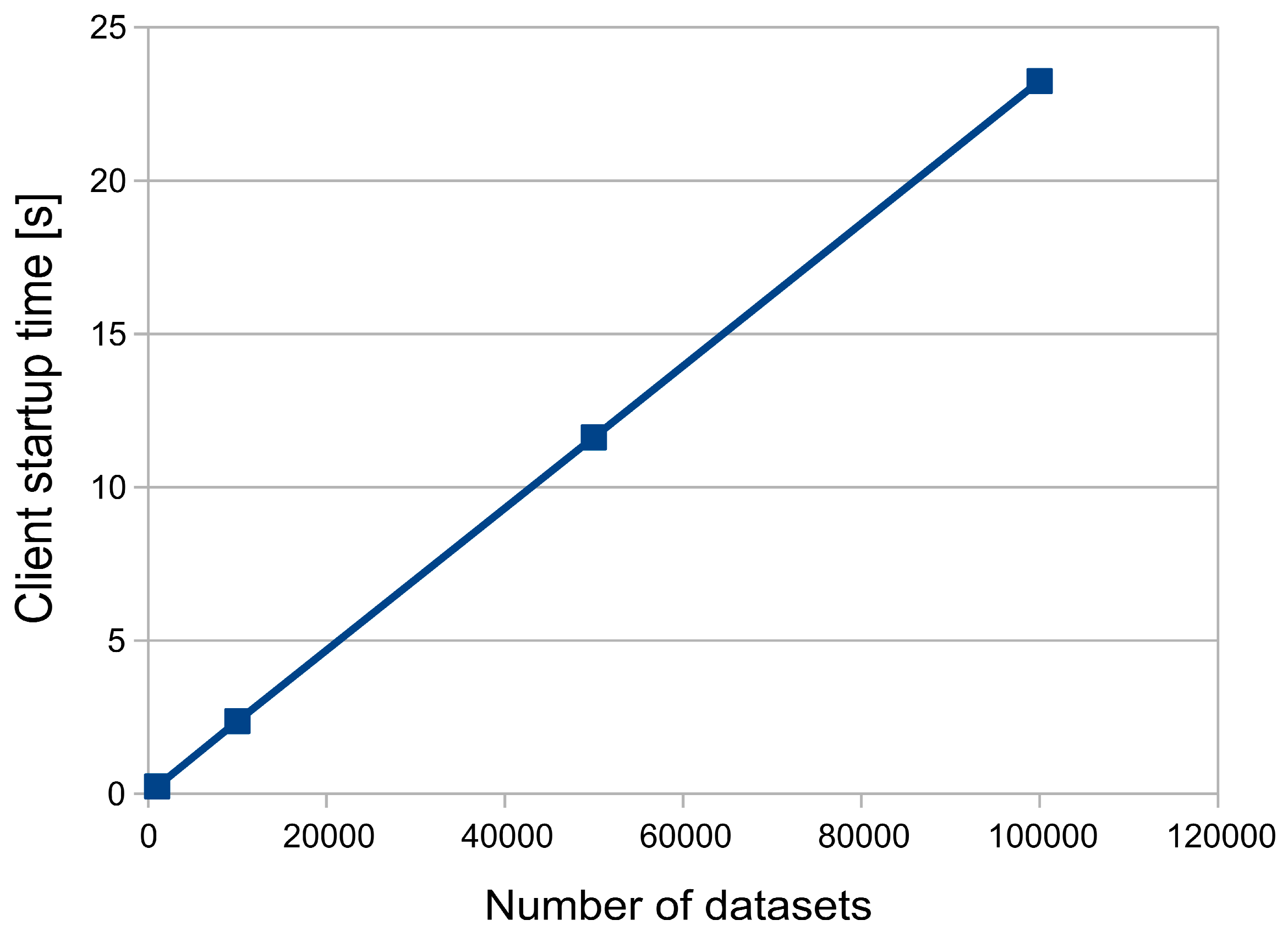
As far as the client startup time is concerned, the system database has been populated with several different numbers of datasets, and the client startup time (which is the time between entering the client website url in the browser and the time when Cesium begins drawing its user interface) has been measured for each database size. Figure 9 presents the results of this.
As expected, the time that is required to generate the layer list linearly scales with the size of the database. For 1000 datasets, it is negligibly short (0.24 s) and only really becomes noticeable at 10 000 datasets, where it takes 2.37 s. While it is difficult to state where the border lies exactly between acceptable and unacceptable delay in application startup time, studies have shown that, when browsing the Web, users may not always be willing to tolerate delays that are longer than several seconds [32]. In this context, it may be said that the wait time for 50 000 datasets (11.63 s) might be somewhat detrimental to user experience. With 100 000 datasets in the database, it takes 23.25 s to generate the list of layers, which is a relatively long time for loading a web page.
As for client performance when displaying large datasets, several different client machines have been tested while using two volumes of data. The first one consisted of roughly 11,000,000 points, while the second one contained over 22,000,000 points. Both of the data volumes have been delivered to the client in the form of 3D Tiles. Similarly to previous client performance tests, the camera has been adjusted to view the entirety of each data volume, and during measurement it has been shifted to the left and right by several pixels while using the Client’s input controls. The test has been performed on machines A, B, and C (which have been described in Section 4.2), however only the built-in discrete Nvidia GeForce 660M GPU has been used on the Laptop machine (B). Moreover, tests that were performed on the Android-powered Smartphone (C) have shown to be problematic due to RAM constraints, and ultimately have not been included in the results. Table 3 presents the latter.
As it can be seen, the Desktop-class PC had little problem displaying even very large volumes of data. When displaying 11,000,000 points, it provided around 50 frames per second, with a memory usage of 544 MB. It was only at 22,000,000 points where its performance significantly decreased, however the delivered 27 frames per second could still provide an acceptable level of user experience. RAM usage was at 950 MB, which was well below the system’s capabilities. However, the Laptop PC shows very different results. Although the tests have been exclusively performed on the higher-performing discrete GPU, when displaying the 11,000,000 points, the system delivered only one frame per second. As expected, the performance was much worse when displaying the 22,000,000 point cloud, where the system required two seconds to render a single frame of animation. RAM usage on the laptop was slightly higher than on the Desktop PC, however this could be an artifact of the browser’s memory management system. As for the Smartphone, when displaying 11,000,000 points, the system RAM was becoming saturated, which was likely the cause of experienced difficulties in rendering the entire point cloud. Because not all of the points were rendered, the phone’s performance metrics have not been included in the results.
As it can be seen, the chosen system architecture presents certain limitations to system performance when serving large amounts of data. With the number of stored datasets exceeding 50 000, the client startup time becomes noticeably long. Moreover, displaying point clouds containing over 20 000 000 points is certainly possible, however it requires a powerful client machine to do so. Smartphones and tablets with less than 6 GB RAM may not be able to properly display a cloud of more than 10 000 000 points. Other limitations of the system in its current form include the already discussed size of a single input file, which may be easily increased with an upgrade of the server’s RAM configuration. Moreover, it should also be noted that, at this point, the system does not allow for the simultaneous processing of multiple datasets. In such cases, the users will need to wait until the processing of the previous dataset has been completed.
5. Conclusions
The application of the presented system to automatic processing, integration, and dissemination of LiDAR survey results has proven the proposed design, architecture, and technological choices to be successful. The system has shown to considerably simplify the process of data organization and integration, while also delivering tools for easy discovery, inspection, and acquisition of desired datasets. Aside from acting as an interactive database, the system may also be used as a hub for data exchange. Third parties could upload their datasets for processing or downloading LiDAR point clouds for their own use. However, most importantly, all data types within the system are stored in open formats and are made available through open protocols. In consequence, any software compatible with those standards may access the contents of the system’s databases. At the same time, the presented system also integrates modern shape reconstruction algorithms, enabling the automated generation of 3D models from source point clouds. Aside from providing a simplified representation of scanned objects in the system, this functionality supports research activities through streamlining the process of testing the reconstruction algorithms. The generated models may be compared to the original point clouds at the click of a button, and in case of issues, the original dataset may be directly downloaded for further investigation. In this context, the presented system has shown to successfully address several issues that are related to LiDAR data management and dissemination.
As far as performance is concerned, the system has been deployed on a single server machine, while regular desktop-class PC’s, Laptops, and Smartphones have been used for running the client. The high optimization of the Cesium library has enabled the operation of the Web-GIS client on an Android-powered smartphone device with good performance. The server has shown to deliver the satisfactory scaling of performance between different hardware configurations and dataset sizes. More importantly, the average data processing times have shown to be several orders of magnitude lower than the time that is required for data collection, which has ensured uninterrupted system operation.
When considering the system limitations, both the maximum size of a single input dataset, as well as the maximum number of features that are displayed by the client have shown to be directly related to the available hardware resources on the server and client, respectively. As such, those limits will continue to shift with the introduction of new and more powerful hardware. The architectural limitations to system scalability include client startup time, which increases along with the size of the system database, as well as the inability to process multiple datasets at the same time. While the latter would require considerable architectural changes to neutralize, the former may be alleviated, for example by presenting visual feedback in the form of a progress bar animation. However, it should be noted that neither of those should pose a serious problem until the number of users (and, in consequence, processed datasets) is significantly increased. Moreover, while the system’s current user interface has been designed for managing a relatively small number of datasets, its functionality can be extended to support large amounts of data e.g., by implementing a mechanism for sorting and grouping datasets in the client by their date of acquisition. In the future, the authors are also planning to provide an option for searching and exploring the datasets by tags that are assigned during the data upload stage.
Summing up, the presented results have shown that the application of open standards of data storage and dissemination, in combination with modern open source GIS libraries, constitutes an efficient tool for integration, processing, and visualization of LiDAR data in a web environment.
Author Contributions
Conceptualization, Marcin Kulawiak and Marek Kulawiak; methodology, Marek Kulawiak and Marcin Kulawiak; software Marek Kulawiak; validation, Marek Kulawiak, Marcin Kulawiak and Zbigniew Lubniewski; formal analysis, Marek Kulawiak and Zbigniew Lubniewski; writing—original draft preparation, Marek Kulawiak and Marcin Kulawiak; writing—review and editing, Marcin Kulawiak and Zbigniew Lubniewski; visualization, Marek Kulawiak.
Funding
This research received no external funding.
Conflicts of Interest
The authors declare no conflict of interest.
References
- ASPRS. LAS Specification Version 1.4; The American Society for Photogrammetry & Remote Sensing: Bethesda, MD, USA, 2011; Available online: http://www.asprs.org/a/society/committees/standards/LAS_1_4_r13.pdf (accessed on 24 January 2019).
- Krishnan, S.; Crosby, C.; Nandigam, V.; Phan, M.; Cowart, C.; Baru, C.; Arrowsmith, R. OpenTopography: A services oriented architecture for community access to LiDAR topography. In Proceedings of the 2nd International Conference on Computing for Geospatial Research & Applications, Washington, DC, USA, 23–25 May 2011; p. 7. [Google Scholar]
- Kuder, M.; Zalik, B. Web-based LiDAR visualization with point-based rendering. In Proceedings of the 2011 Seventh International Conference on Signal-Image Technology and Internet-Based Systems (SITIS), Dijon, France, 28 November–1 December 2011; pp. 38–45. [Google Scholar]
- Lewis, P.; Mc Elhinney, C.P.; McCarthy, T. LiDAR data management pipeline; from spatial database population to web-application visualization. In Proceedings of the 3rd International Conference on Computing for Geospatial Research and Applications, Washington, DC, USA, 1–3 July 2012; p. 16. [Google Scholar]
- Mao, B.; Cao, J. HTML5 Based 3D Visualization of High Density LiDAR Data and Color Information for Agriculture Applications. In Social Media Retrieval and Mining; Springer: Berlin/Heidelberg, Germany, 2013; pp. 143–151. [Google Scholar]
- Maravelakis, E.; Konstantaras, A.; Kabassi, K.; Chrysakis, I.; Georgis, C.; Axaridou, A. 3DSYSTEK web-based point cloud viewer. In Proceedings of the IISA 2014, 5th International Conference on Information, Intelligence, Systems and Applications, Chania Crete, Greece, 7–9 July 2014. [Google Scholar]
- Nale, A. Design and Development of a Generalized LiDAR Point Cloud Streaming Framework over the Web. Master’s Thesis, Università degli Studi di Padova, Padova, Italy, 2014. [Google Scholar]
- Li, Z.; Hodgson, M.E.; Li, W. A general-purpose framework for parallel processing of large-scale LiDAR data. Int. J. Digit. Earth 2018, 11, 26–47. [Google Scholar] [CrossRef]
- von Schwerin, J.; Richards-Rissetto, H.; Remondino, F.; Spera, M.G.; Auer, M.; Billen, N.; Loos, L.; Stelson, L.; Reindel, M. Airborne LiDAR acquisition, post-processing and accuracy-checking for a 3D WebGIS of Copan, Honduras. J. Archaeol. Sci. Rep. 2016, 5, 85–104. [Google Scholar] [CrossRef] [Green Version]
- Schmiemann, J.; Harms, H.; Schattenberg, J.; Becker, M.; Batzdorfer, S.; Frerichs, L. A distributed online 3D-lidar mapping system. Int. Arch. Photogramm. Remote Sens. Spat. Inf. Sci. 2017, 42, 339. [Google Scholar] [CrossRef]
- Huang, J.; Wang, J. 3D Visualization of Point Clouds Using HTML5 and WebGL. In Proceedings of the 2017 7th International Conference on Computer Engineering and Networks, Shanghai, China, 22–23 July 2017. [Google Scholar]
- Bohak, C.; Kim, B.H.; Kim, M.Y. Web-based real-time ladar data visualization with multi-user collaboration support. In Proceedings of the International Conference on Augmented Reality, Virtual Reality and Computer Graphics, Otranto, Italy, 24–27 June 2018; Springer: Cham, Switzerland, 2018; pp. 214–224. [Google Scholar]
- GeoSignum BV Products Information, Web-Based LiDAR Data Processing. Available online: https://geosignum.nl/index.php/product-services/pointer-cloud-software (accessed on 17 January 2019).
- De la Beaujardiere, J. (Ed.) OpenGIS Web Map Service (WMS) Implementation Specification ver.1.3.0. 2006. Available online: http://www.opengeospatial.org/standards/wms (accessed on 6 January 2019).
- Vretanos, P.A. (Ed.) OpenGIS Web Feature Service (WFS) Implementation Specification ver. 1.1. 2005. Available online: http://www.opengeospatial.org/standards/wfs (accessed on 6 January 2019).
- Gröger, G.; Kolbe, T.H.; Nagel, C.; Häfele, K.-H. (Eds.) OGC City Geography Markup Language (CityGML) Encoding Standard. 2012. Available online: http://www.opengeospatial.org/standards/citygml (accessed on 6 January 2019).
- Prandi, F.; Devigili, F.; Soave, M.; Di Staso, U.; De Amicis, R. 3D web visualization of huge CityGML models. Int. Arch. Photogramm. Remote Sens. Spat. Inf. Sci. 2015, 40, 601–605. [Google Scholar] [CrossRef]
- ESRI Scene Layers: Service and Package Standard. Available online: https://github.com/Esri/i3s-spec (accessed on 14 January 2019).
- 3D Tiles Specification. Available online: https://github.com/AnalyticalGraphicsInc/3d-tiles (accessed on 14 January 2019).
- Kulawiak, M.; Kulawiak, M. Application of Web-GIS for Dissemination and 3D Visualization of Large-Volume LiDAR Data. In The Rise of Big Spatial Data; Springer: Cham, Switzerland, 2017; pp. 1–12. [Google Scholar] [CrossRef]
- OGC Seeks Public Comment on 3D Tiles Candidate Community Standard. Available online: https://www.opengeospatial.org/pressroom/pressreleases/2829 (accessed on 14 January 2019).
- Mustafa, A.; Wei Zhang, X.; Aliaga, D.G.; Bruwier, M.; Nishida, G.; Dewals, B.; Erpicum, S.; Archambeau, P.; Pirotton, M.; Teller, J. Procedural generation of flood-sensitive urban layouts. Environ. Plan. B Urban Anal. City Sci. 2018, 1–23. [Google Scholar] [CrossRef]
- Sitnik, R.; Karaszewski, M. Optimized point cloud triangulation for 3D scanning systems. Mach. Graph. Vis. 2008, 17, 349–371. [Google Scholar]
- Kulawiak, M.; Łubniewski, Z. 3D Object Shape Reconstruction from Underwater Multibeam Data and Over Ground Lidar Scanning. Pol. Marit. Res. 2018, 25, 47–56. [Google Scholar] [CrossRef]
- Kulawiak, M.; Lubniewski, Z. Processing of LiDAR and Multibeam Sonar Point Cloud Data for 3D Surface and Object Shape Reconstruction. In Proceedings of the Baltic Geodetic Congress (Geomatics), Gdansk, Poland, 2–4 June 2016; pp. 187–190. [Google Scholar] [CrossRef]
- Kazhdan, M.; Hoppe, H. Screened poisson surface reconstruction. ACM Trans. Graph. (ToG) 2013, 32, 29. [Google Scholar] [CrossRef]
- Cignoni, P.; Callieri, M.; Corsini, M.; Dellepiane, M.; Ganovelli, F.; Ranzuglia, G. Meshlab: An open-source mesh processing tool. In Proceedings of the Eurographics Italian Chapter Conference, Salerno, Italy, 2–4 July 2008; Volume 2008, pp. 129–136. [Google Scholar] [CrossRef]
- Reddy, M. OBJ Format Specification. Available online: http://www.martinreddy.net/gfx/3d/OBJ.spec (accessed on 24 January 2019).
- An Open-Source JavaScript Library for World-Class 3D Globes and Maps. Available online: https://cesiumjs.org/ (accessed on 14 January 2019).
- Sentinel-2 Cloudless Map of the World. Available online: https://s2maps.eu/ (accessed on 14 January 2019).
- Moszynski, M.; Kulawiak, M.; Chybicki, A.; Bruniecki, K.; Bieliński, T.; Łubniewski, Z.; Stepnowski, A. Innovative web-based geographic information system for municipal areas and coastal zone security and threat monitoring using EO satellite data. Mar. Geod. 2015, 38, 203–224. [Google Scholar] [CrossRef]
- Nah, F.F.H. A study on tolerable waiting time: How long are web users willing to wait? Behav. Inf. Technol. 2004, 23, 153–163. [Google Scholar] [CrossRef]
Figure 1.
Architecture of the system for online processing, storage, visualization and dissemination of Light Detection and Ranging (LiDAR) survey results.
Figure 1.
Architecture of the system for online processing, storage, visualization and dissemination of Light Detection and Ranging (LiDAR) survey results.

Figure 2.
The system’s Data upload service.

Figure 3.
When data processing completes, the Data upload module redirects the user to the Web-.

Figure 4.
The system’s Web-based Geographic Information System (Web-GIS) client displaying a model reconstructed from the processed dataset.
Figure 4.
The system’s Web-based Geographic Information System (Web-GIS) client displaying a model reconstructed from the processed dataset.

Figure 5.
The system’s Web-GIS client displaying the original point cloud of the processed dataset.

Figure 6.
The system’s Web-GIS client displaying three-dimensional (3D) meshes of the Gdansk University of Technology Faculty of Electronics, Telecommunications, and Informatics on a Snapdragon 835 smartphone.
Figure 6.
The system’s Web-GIS client displaying three-dimensional (3D) meshes of the Gdansk University of Technology Faculty of Electronics, Telecommunications, and Informatics on a Snapdragon 835 smartphone.

Figure 7.
Scaling of processing time in relation to size of input data.

Figure 8.
Scaling of RAM consumption in relation to size of input data.

Figure 9.
Scaling of client startup time in relation to size of database.


Table 1.
The measured processing time and RAM consumption for every processed dataset.
| Dataset | Processing Time [s] | RAM Usage [MB] |
|---|---|---|
| Point cloud A | 75.9 | 429.2 |
| Point cloud B | 49.2 | 339.8 |
| Point cloud C | 18.3 | 221.2 |
| Point cloud D | 4.9 | 162.2 |
Table 2.
The measured performance characteristics of the Web-GIS client running on different machines.
Table 2.
The measured performance characteristics of the Web-GIS client running on different machines.
| Machine | FPS | RAM Usage | CPU Use |
|---|---|---|---|
| Machine A | 60 | 175 MB | 15% (60% of 1 core) |
| Machine B | 15 (55) 1 | 176 MB | 7% (60% of 1 core) |
| Machine C | 25 | 298 MB | 28% (100% of 1 core) |
1 Performance measured when using the built-in GeForce 660M Graphic Processing Unit (GPU).
Table 3.
The performance of large-volume data visualization on different machines.
| Machine | 11 Million Points | 22 Million Points | ||
|---|---|---|---|---|
| FPS | RAM Usage | FPS | RAM Usage | |
| Machine A | 50 | 544 MB | 27 | 950 |
| Machine B | 1 | 550 MB | 0.5 | 990 |
© 2019 by the authors. Licensee MDPI, Basel, Switzerland. This article is an open access article distributed under the terms and conditions of the Creative Commons Attribution (CC BY) license (http://creativecommons.org/licenses/by/4.0/).
Share and Cite
MDPI and ACS Style
Kulawiak, M.; Kulawiak, M.; Lubniewski, Z. Integration, Processing and Dissemination of LiDAR Data in a 3D Web-GIS. ISPRS Int. J. Geo-Inf. 2019, 8, 144. https://doi.org/10.3390/ijgi8030144
AMA Style
Kulawiak M, Kulawiak M, Lubniewski Z. Integration, Processing and Dissemination of LiDAR Data in a 3D Web-GIS. ISPRS International Journal of Geo-Information. 2019; 8(3):144. https://doi.org/10.3390/ijgi8030144
Chicago/Turabian StyleKulawiak, Marek, Marcin Kulawiak, and Zbigniew Lubniewski. 2019. "Integration, Processing and Dissemination of LiDAR Data in a 3D Web-GIS" ISPRS International Journal of Geo-Information 8, no. 3: 144. https://doi.org/10.3390/ijgi8030144
Note that from the first issue of 2016, this journal uses article numbers instead of page numbers. See further details here.