Article

Application of Ordinary Kriging and Regression Kriging Method for Soil Properties Mapping in Hilly Region of Central Vietnam

by
Tung Gia Pham
1,2,*,
Martin Kappas
1,
Chuong Van Huynh
3 and
Linh Hoang Khanh Nguyen
4
1
Cartography, GIS and Remote Sensing Department, Göttingen University, 37077 Göttingen, Germany
2
Faculty of Land Resources and Agricultural Environment, University of Agriculture and Forestry, Hue University, 0234 Hue, Vietnam
3
Presidential Board, Hue University, 0234 Hue, Vietnam
4
International School, Hue University, 0234 Hue, Vietnam
*
Author to whom correspondence should be addressed.
ISPRS Int. J. Geo-Inf. 2019, 8(3), 147; https://doi.org/10.3390/ijgi8030147
Submission received: 13 February 2019 / Revised: 11 March 2019 / Accepted: 15 March 2019 / Published: 19 March 2019

Abstract

:
Soil property maps are essential resources for agricultural land use. However, soil properties mapping is costly and time-consuming, especially in the regions with complicated topographic conditions. This study was conducted in a hilly region of Central Vietnam with the following objectives: (i) to evaluate the best environmental variables to estimate soil organic carbon (SOC), total nitrogen (TN), and soil reaction (pH) with a regression kriging (RK) model, and (ii) to compare the accuracy of the ordinary kriging (OK) and RK methods. SOC, TN, and soil pH data were measured at 155 locations within the research area with a sampling grid of 2 km × 2 km for a soil layer from 0 to 30 cm depth. From these samples, 117 were used for interpolation, and the 38 randomly remaining samples were used for evaluating accuracy. The chosen environmental variables are land use type (LUT), topographic wetness index (TWI), and transformed soil adjusted vegetation index (TSAVI). The results indicate that the LUT variable is more effective than TWI and TSAVI for determining TN and pH when using the RK method, with a variance of 7.00% and 18.40%, respectively. In contrast, a combination of the LUT and TWI variables is the best for SOC mapping with the RK method, with a variance of 14.98%. The OK method seemed more accurate than the RK method for SOC mapping by 3.33% and for TN mapping by 10% but the RK method was found more precise than the OK method for soil pH mapping by 1.81%. Further selection of auxiliary variables and higher sampling density should be considered to improve the accuracy of the RK method.

1. Introduction

Soil quality information plays a vital role in land use planning, resource management and site investigation [1]. The most popular indicators to assess soil quality are soil organic carbon (SOC), total nitrogen (TN) and soil reaction (pH) [2,3]. The SOC is one of the most important indicators of soil quality for agricultural land use due to its impact on physical, chemical and biological indicators of soil quality, such as soil texture, nutrient availability in soil or electrical conductivity [4]. Moreover, TN and pH have an impact on growth of plants [5,6]. Reliable information on the spatial distribution of these soil quality indicators is required for sustainable land management and agricultural production [7,8].
There are various methods for interpolation of spatial distribution of SOC, TN and soil pH, such as inverse distance weighting (IDW) and ordinary kriging (OK) [9,10,11,12,13]. In recent years, researchers have suggested a combination of regression and spatial interpolation, called regression kriging (RK), to determine the spatial distribution of soil characteristics [14,15,16,17,18,19,20,21]. For this method, the selection of auxiliary variables is essential and remotely sensed images are typically the first choice [22]. The OK has been widely used in interpolation techniques due to its simplicity as well as availability in many geographical information systems (GISs) [23,24]. In recent years, RK has become an acceptable method for soil mapping due to its lower cost, and its accuracy often outperforms other methods [25]. However, the accuracy of the RK method is not clear in all of the case studies because it depends on actual soil and environmental variable relationships [26].
For soil characteristic mapping based on environmental variables, researchers [27] often use terrain characteristics as independent variables [19,27,28]. Some researchers use the topographic wetness index (TWI), a local scale index to quantitatively indicate the balance between water accumulation and drainage conditions, as an environmental variable for SOC mapping [29,30,31] or TN mapping [16,27].
Most researchers [17,18,31,32,33], however, use normalized difference vegetation index (NDVI) as an auxiliary variable for the regression process. NDVI has been applied to many different aspects of rangeland ecology, but it has limitations. Huete and Jackson [34] found that the soil surface impact on NDVI value was the most significant in areas with a vegetation cover between 45% and 70%. Moreover, NDVI is an estimate of above ground biomass, so if the vegetation is sparse with bare soil present, the soil color may significantly influence the spectral signal. Xue and Su [35] stated that when background brightness is increased, the NDVI also increases. To cope with these inconveniences, Baret et al. [36] suggested an index, the TSAVI, to minimize the soil brightness effect.
LUT is also considered an environmental variable for SOC and TN mapping [37], as well as soil pH mapping [38]. At the current research site, Pham et al. [39] stated that different land use systems significantly influence the SOC, TN, and pH.
Mountains and hills cover eighty percent of Vietnam’s territory with a complicated terrain. However, eighty-five percent of it are low mountains and hills. The landscape of Central Vietnam is a narrow shape with the hills in the West and small plains along the coast. Among the three macro-regions of Vietnam, the Central region is the least developed [40]. The agricultural and forested land areas of the Central region account for seventy-eight percent of the total area [41], and the agricultural production is the main livelihood of local inhabitants. The lack of soil properties information is one of the main obstacles for agricultural cultivation in Central Vietnam [42]. Therefore, this study conducted in the A Luoi district of Vietnam, aimed (i) to evaluate the best environmental variables to estimate SOC, TN, and soil pH with RK model, and (ii) compare the accuracy of the OK and RK method for soil property mapping.

2. Materials and Methods
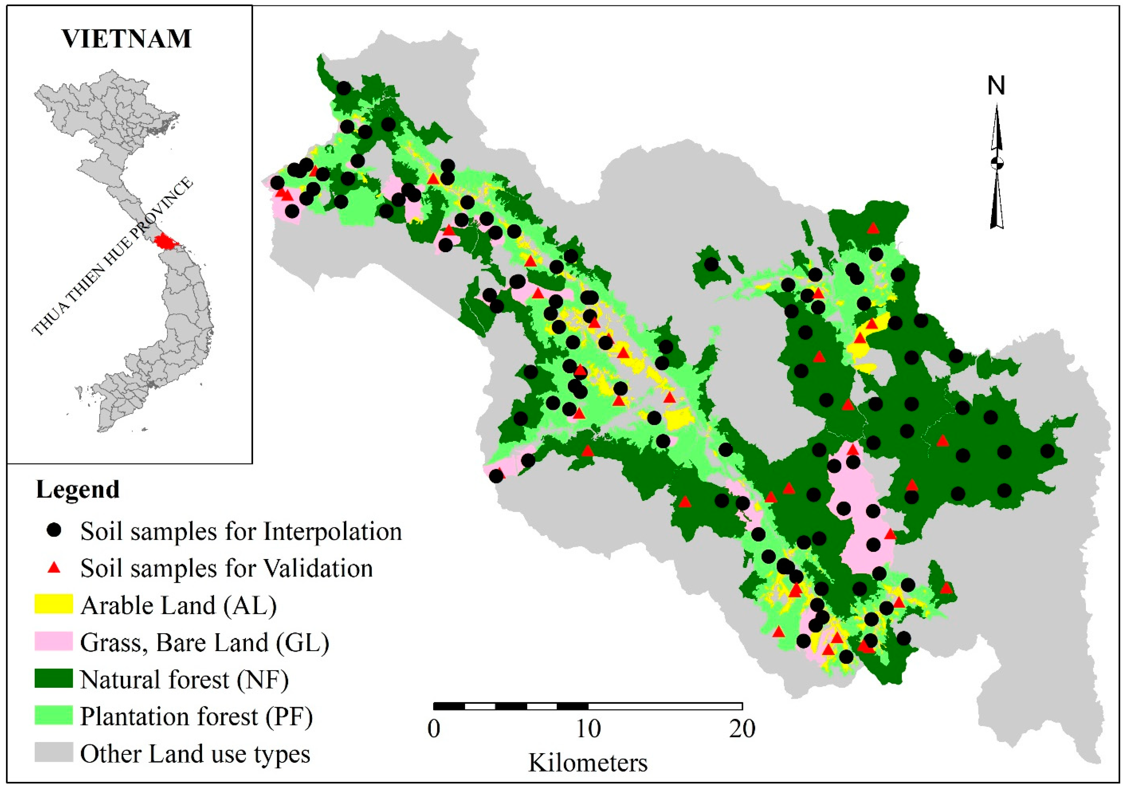
2.1. Research Area

The study area is located between 107°E to 107°30′E and 16°N to 16°30′N, approximately 60 km west of Hue City, in the low mountainous and hilly region of Central Vietnam. Agricultural production, the collection of forest products, and social subsidies provide the main livelihood for the local people. The lack of primary resources, such as finance and market access, present challenges to these local communities.
The climate at the research site exhibits tropical monsoon characteristics with an annual rainy season from September to December. According to statistics from 2005 to 2015, the average yearly precipitation is approximately 3180 mm. The average temperature is the highest in May at 25 °C, while the lowest is in January at 17 °C [43]. The research site has a mountainous topography, with an elevation between 60 and 1760 m above sea level, which decreases from west to east. The slope of the terrain is complex and steep with an average slope of ten degrees. There are four soil types within the research site: Ferralic Acrisols (75%), Arenic Acrisols (14%), Humic Acrisols (6%), and Hyperdystrict Acrisols (5%). Regarding the soil texture, loam is major (71%), followed by silt loam (24%) and clay loam (5%) [44].
The total area of the A Luoi district is 122,415 hectares (ha), comprising 61,105 ha (49%) of protected forests, 57,492 ha (47%) of agricultural land, 2318 ha (2%) of water bodies and 2500 ha (2%) of residential and commercial area [45].

2.2. Remote Sensing Data

In this research, the near-infrared (NIR) and red bands were extracted from Landsat 8 data, which were downloaded from the United States Geological Survey (USGS) (acquired on 24 January 2015 with cloud cover less than 10%). The data were atmospherically corrected and converted from digital numbers to reflectance values by dark object subtraction (DOS1) algorithm and top of atmosphere reflectance (TOA) tool in QGIS software version 3.2 before calculation of the soil line [46]. The digital elevation model (DEM) was downloaded from USGS and used for calculating the TWI. The data were stored in raster format with a spatial resolution of 30 m.

2.3. Field Survey and Soil Quality Analysis

The samples were collected in December 2015 relying on soil unit maps at scale 1:100000 and the grid sampling method. Soil unit maps display the soil type, land use, and slope [44,45]. In total, 78 soil units are present at the research site. A grid sampling of 2 km × 2 km size for general cases and 4 km × 4 km for large areas and highly homogeneous areas was carried out. The guideline for sampling follows two basic principles: (1) if only one soil unit exists in the grid cell, the sample will be taken at the center of the cell, or (2) if more than one soil unit exists, the sample will be taken at the center for each unit that covers an area bigger than 30 ha in that grid. For each sample, soil material in the layer at 0–30 cm was collected from five points (North, South, East, West, and Center) inside a circle with a radius of 25 m then mixed together as a soil sample. A total of 155 soil samples were collected, air-dried and passed through a 2 mm sieve to remove stones, grass, forest litter and any other material on the soil surface. Out of these, 117 samples were used for spatial interpolation, and the 38 remaining samples (25% of total number samples) were used for validation of the model [47,48,49]. Figure 1 shows the locations of the soil samples. SOC was determined with the Walkley–Black method [50], TN was determined via Kjeldahl’s digestion [51,52], and pH was measured using a portable pH meter and 1M KCl [53]. The samples were analyzed at the laboratory of the Soil Science Department at the Hue University of Agriculture and Forestry, in Vietnam.

2.4. Environmental Variables Data

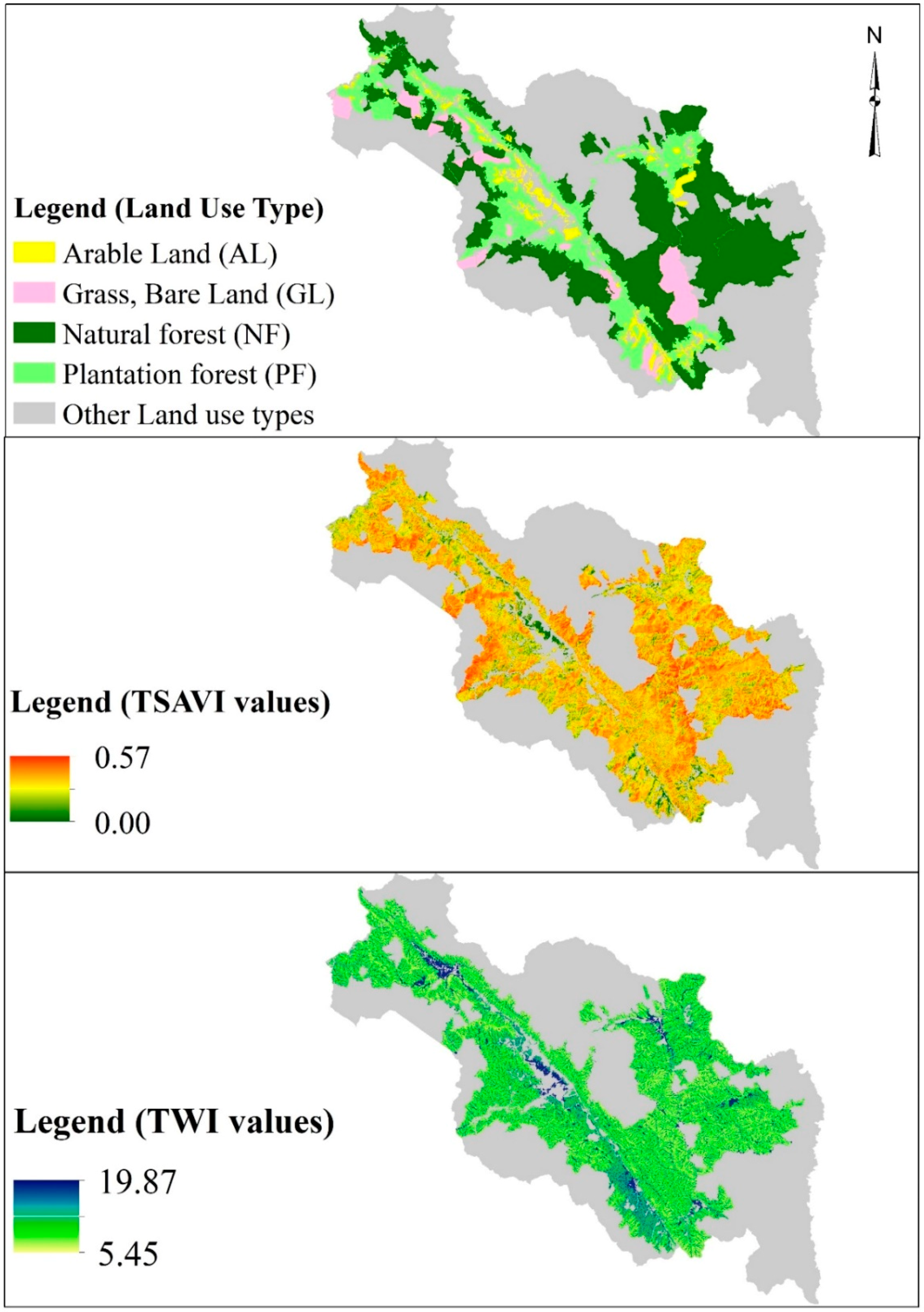
2.4.1. Transformed Soil Adjusted Vegetation Index (TSAVI)

Baret et al. [36] proposed the TSAVI to minimize the effect of the soil background [54]. Baret and Guyot [55] defined TSAVI with the following equation:
TSAVI = α ( NIR α R β ) ( R + α ( NIR β ) + X ( 1 + α 2 ) )
The soil line represents the relationship between the red (R) and near-infrared (NIR) reflectances of bare soil that was proposed by Richardson and Wiegand [56], modeled with the following equation:
NIR = α R + β
In Equation (1) and (2), α and β are the slope and intercept of the soil line, respectively, NIR is the near-infrared, R is the red reflectance value, and X is soil background adjustment factor (almost in all cases X is 0.08). TSAVI equals zero for bare soil and is close to one for very high leaf area indices.
The soil line extends from an upper value of bright soil with high reflectance in both the R and NIR bands to lower values for darker soils [57]. In this study, the soil line was identified with the quantile regression method. The quantile was set at a number close to zero, for example, 0.00001 [54].

2.4.2. Topographic Wetness Index (TWI)

TWI proposed by Beven and Kirkby [58], also called the compound topographic index, is based on two parameters: upstream contributing area and slope. TWI is represented as:
TWI = ln ( λ tan δ )
where λ is the contributing area and δ is the local slope of the terrain. High values of TWI indicate a high potential for runoff generation. TWI is unitless. In this study, TWI was calculated with the aid of the raster calculator tool in ArcGIS 10.5.

2.5. Spatial Interpolation

2.5.1. Ordinary Kriging

OK is one of the most commonly used kriging techniques. The spatial prediction of the unmeasured point xo is given by predicting the value Z ( x o ) , which equals the line sum of the known measured values (i.e., observed values). Isaaks and Srivastava [59], Cressie [60] and many other researchers provide an elegant and simple description of OK as the following formula:
Z ( x o ) = i = 1 n λ i Z ( x i )
where Z ( x o ) is the predicted value at the unmeasured position xo, Z ( x i ) is the measured value at position xi, λi is the weighting coefficient from the measured position to xo and n is the number of positions within the neighborhood searching [61]. A fitted model based on the input data distribution is needed to describe the spatial continuity of the data and show the spatial relationship between the pairs of points. In this study, the OK method was calculated using R software with a framework introduced by Hengl [61] and Omuto and Vargas [62].

2.5.2. Regression Kriging
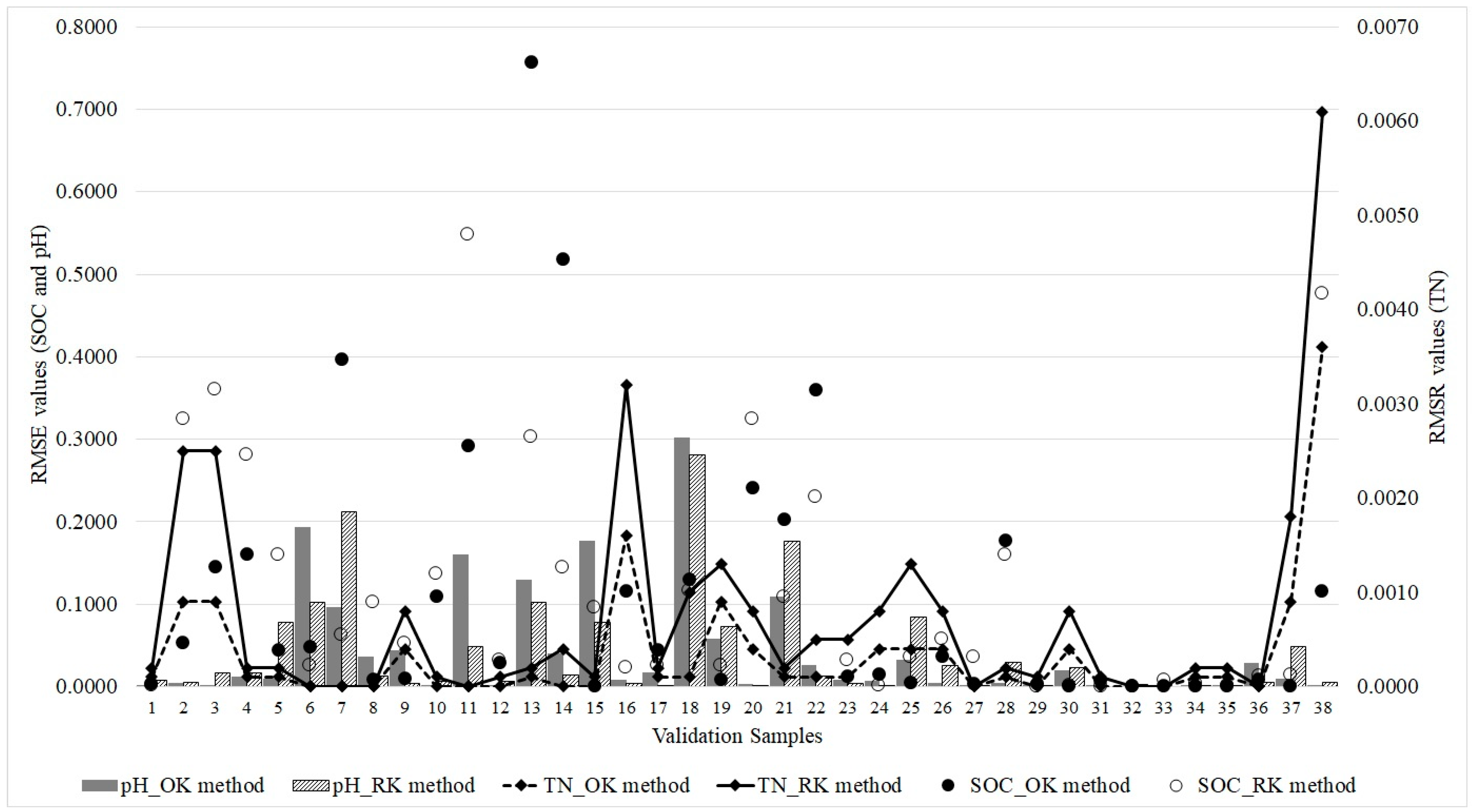
RK is a spatial interpolation technique that combines a regression of dependent variables on predictors with kriging of the prediction residuals [14,63]. The following equation calculates the RK interpolation:
Z ( x o ) = m ^ ( x o ) + e ^ ( x o ) = k = 0 p β ^ k q k ( x o ) + i = 1 n λ i e ( x i )
where m ^ ( x o ) is the fitted deterministic part, e ^ ( x o ) is the interpolated residual, β ^ k are the estimated deterministic model coefficients, λi are the kriging weights determined by the spatial dependence structure of the residual and e(xi) is the residual at position xi. Thus, the first part of the right-hand side of Equation (5) represents the regression and the second part represents the kriging of the residual. Hengl et al. [14] introduced the process of using the RK method for spatial prediction of soil variables. In this study, RK was conducted using the R software [64,65,66] with a framework introduced by Hengl [61] and Omuto and Vargas [62].

2.6. Validation

Thirty-eight of the 155 soil samples were randomly extracted from the dataset to test the predictive accuracy of the model. This was evaluated by comparing the observed and predicted SOC, TN, and pH values at validation point locations. In this study, mean error (ME) and root mean square error (RMSE) were selected as validation indices. We used RI to compare the OK and RK methods and to improve the prediction accuracy index. If RI is positive, the accuracy prediction of RK is higher than that of OK and vice-versa [16].
ME = 1 n j = 1 n ( Z o i Z p i )
RMSE = 1 n j = 1 n ( Z o i Z p i ) 2
R I = RMSE OK RMSE RK RMSE OK 100 %
In Equations (6)–(8), ME is mean error, RMSE is root mean square error, n is the number of testing points, Zoi is the observed value at the ith position, and Zpi is the predicted value at the ith position.

3. Results

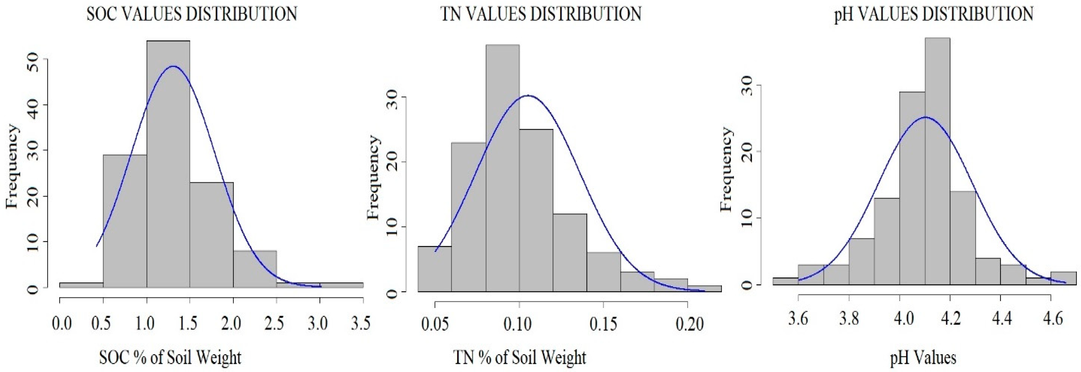
3.1. Soil Samples Data Descriptions

The percent SOC of the topsoil layer (0-30 cm depth) varies from 0.42% to 3.02%. Meanwhile, TN ranges from 0.05% to 0.21%, and pH ranges from 3.60 to 4.68 (Table 1). High standard deviation values of SOC and TN (compared to the mean of each soil quality indicator value) imply that these values are widely distributed, while low standard deviation values indicate most of the values are close to an average value. The differences in SOC and TN between the samples were substantial, and vice versa for the soil pH. The distributions of all variables were only slightly skewed (with a skewness value less than 1.0), and their median values were very close to the mean values. Therefore, the soil property values of the sampling points follow a normal distribution (Figure 2).

3.2. Regression Model for Soil Characteristics Mapping

3.2.1. Environmental Variables Calculation

LUT, TSAVI, and TWI are predictor variables (independent variables) in this research. Figure 3 shows the spatial distribution of these variables. Based on the 2015 land use map [45], scale 1:50000 and the field survey results, we determined four LUTs belonging to the agricultural land use categories were arable land (AL), grassland (GL), natural forest (NF) and plantation forest (PF). The slope and intercept value of the soil line (α = 1.026, β = 0.00003) was determined for the research site. Using Equation (4), the TSAVI ranges from 0 to 0.57. The TSAVI values of AL are lower than for other land use types. The TWI value of the research site changes from 5.4 to 19.87. Most of the area of GL, PF, and NF have TWI values of approximately 10, while the TWI values of AL are higher than those of other land use types.

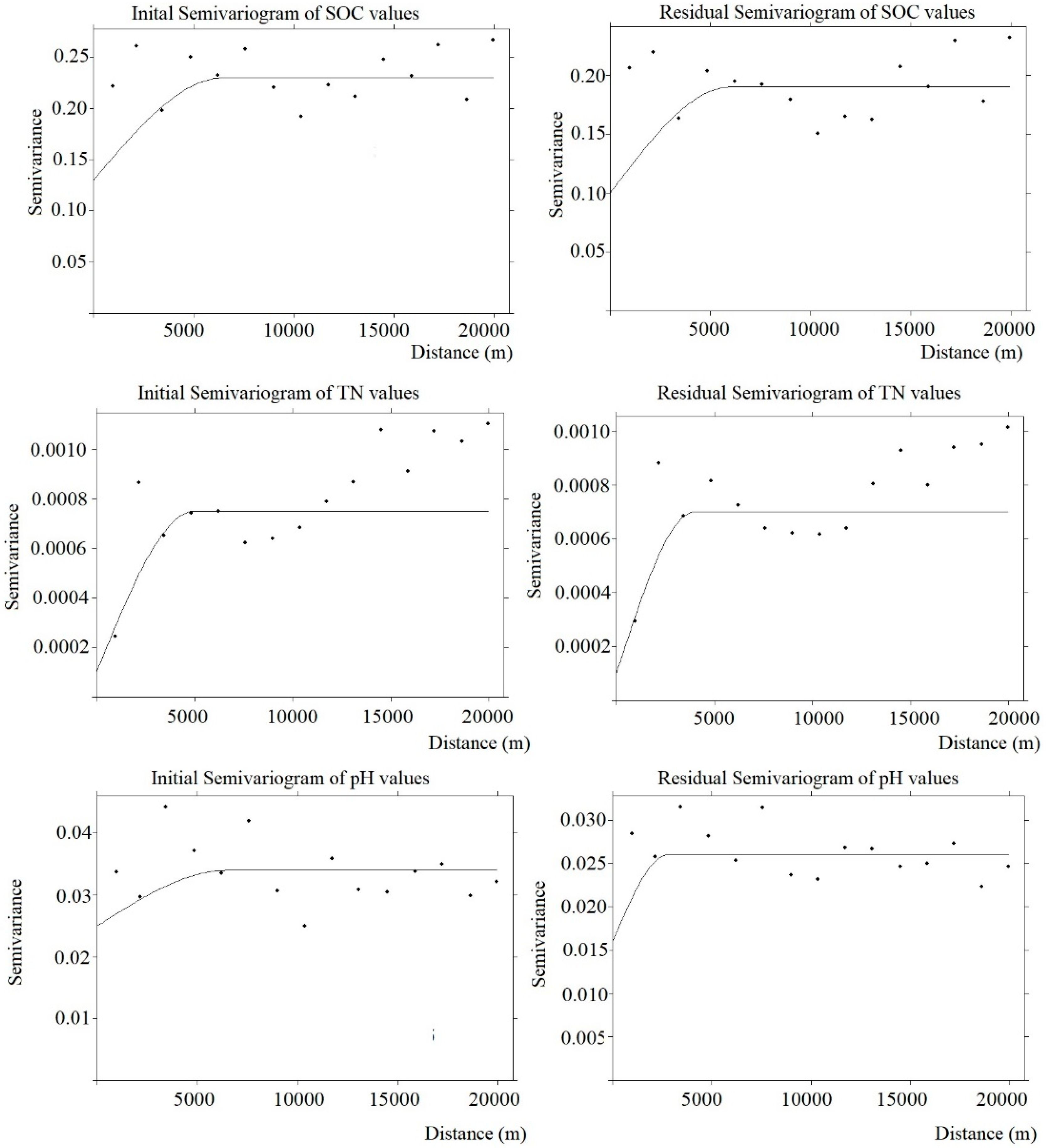
3.2.2. Model for Regression Kriging

Adjusted R squared values are critical to explaining the influence of the independent variables on the dependent variables of the model. The results from Table 2 show that the LUT affects TN and pH (7.00% for TN, 18.40% for pH), whereas a combination of the LUT and the TWI has the most robust impact on the SOC with a variance of 14.98%. Environmental variables affect SOC and soil pH more than they affect TN. Therefore, y = f(LUT) was used for TN and pH mapping with the RK method, while y = f(TWI, LUT) was used for SOC interpolation.
The semivariogram depicts the spatial autocorrelation of the measured sample points. Figure 4 and Table 3 show the semivariogram and residual semivariogram of SOC, TN, and pH data. Both semivariogram models (initial variables and residuals) have approximately the same form, but the residuals semivariogram model has a small difference in sill, nugget, and range.
The nugget parameter of the SOC semivariogram is very high, meaning that the unexplained variability of this soil indicator is caused by measurement error rather than the short sampling distance. Moreover, the nugget/sill ratio of SOC and pH is 0.56 and 0.86, respectively, indicating that the sampled spatial dependence is weak. This ratio indicates that the SOC value errors are related to sampling distances. The nugget/sill ratio of TN is lower than the ratio of other soil indicators. Since the nugget value is higher than zero, the separated observation by the smallest distances is dissimilar.

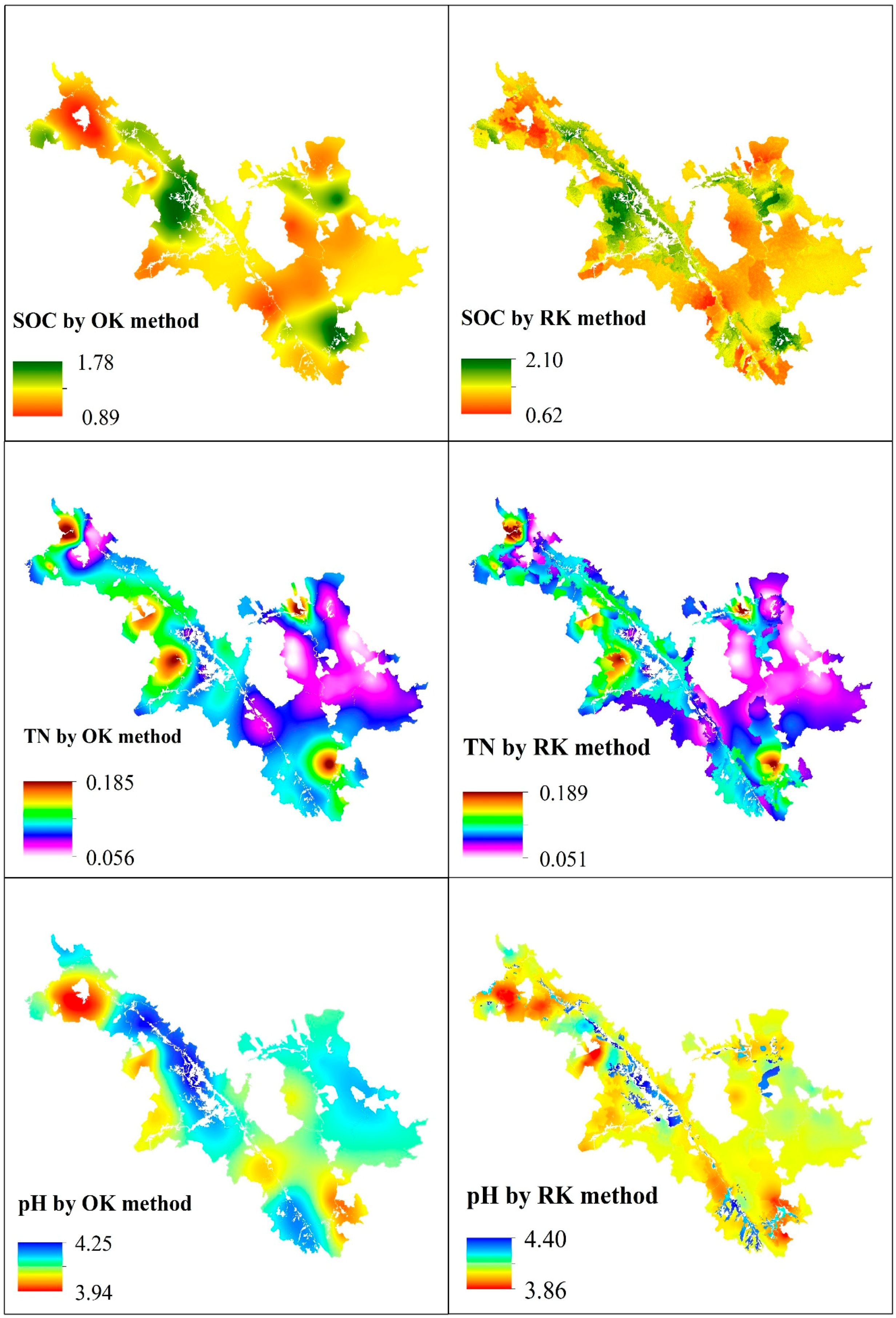
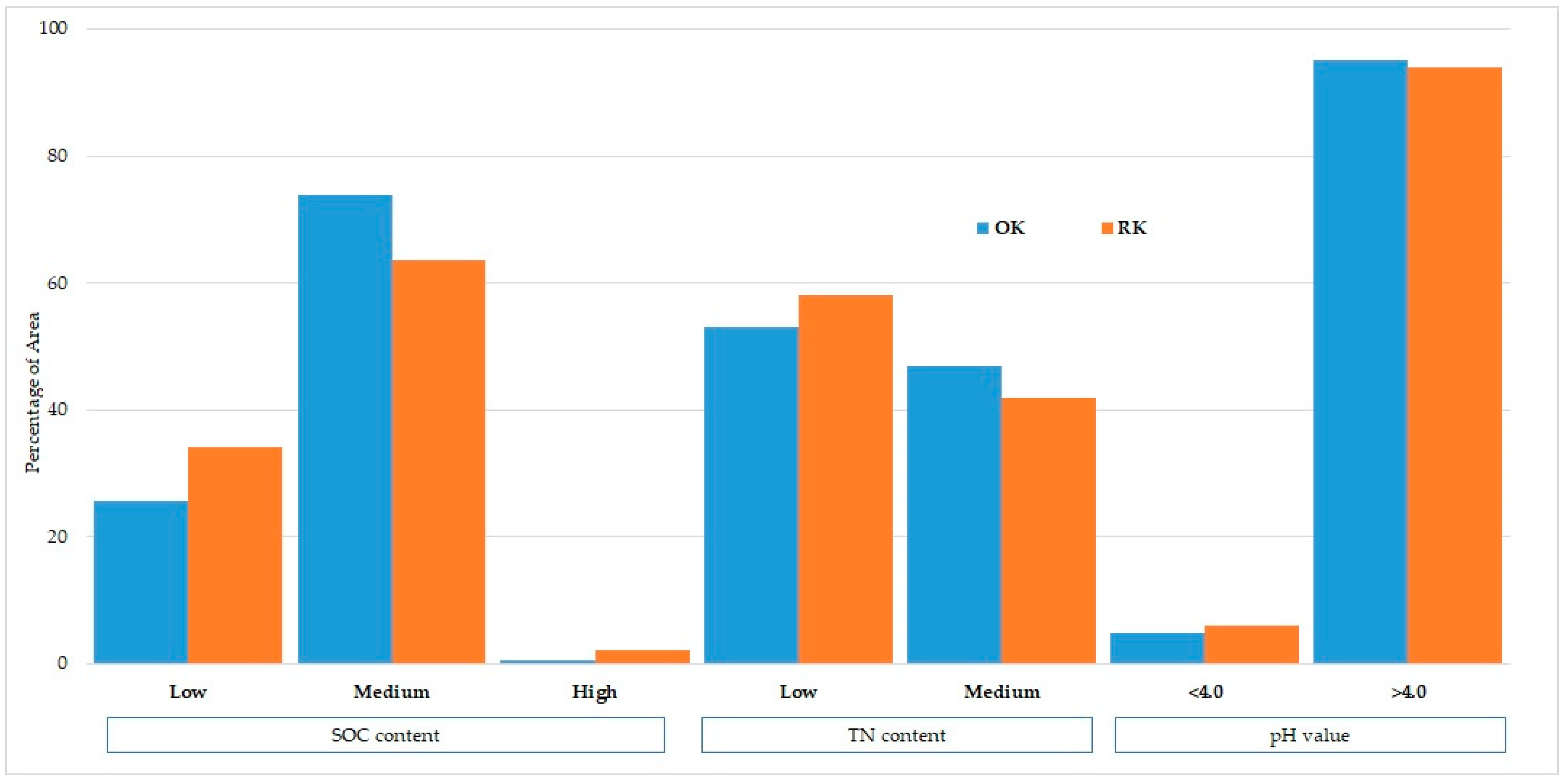
3.3. Spatial Interpolation

The spatial prediction maps by OK and RK method are presented in Figure 5 for the SOC, TN, and soil pH indicators. The SOC at the research site ranges from 0.89% to 1.78% when interpolated with the OK method. When interpolated with the RK method, the SOC content is somewhat more detailed than the OK method, ranging from 0.62% to 2.10%. The pH varies from 3.94 to 4.25 for the OK method and from 3.86 to 4.40 for the RK method. The TN for both methods does not differ much, 0.051 for the lowest threshold and nearly 0.189 for the highest value. The OK prediction map shows the gradual transition of the detailed level is lower than the transition with the RK method. The influence of auxiliary variables is shown clearly on the maps, which was interpolated with the RK method. For the TN and pH maps, transitions are evident at the boundaries between land use types, however, these changes are recorded at different TWI value locations and boundaries between different land use types on the SOC map as well.
According to SOC classification by Le and Ton, cited in Nguyen and Klinnert [67], SOC in upland soil in Vietnam was divided into three groups (less than 0.58% is low, from 0.58 to 1.16 is medium, and more than 1.74% is high). Regarding the TN, Do and Nguyen [68] suggested three groups for Vietnamese soil (less than 0.1 is low, from 0.1 to 0.2% is medium, and more than 0.2% is high). The results (Figure 6) show that there are small differences between the maps obtained by the OK and RK methods. The percentage of area where SOC ranges from 1.16% to 1.74% (medium level) by the OK method is 9% higher than by the RK method, and vice-versa for the remaining SOC contents. Meanwhile, there are more TN values at a low level when interpolated by the RK method compared to the OK method (58% and 53% of the total area, respectively). The difference in the percentage of area for pH values between the RK and the OK method is not significant. In general, the distributions of soil property classes in maps created by both methods are the same.
For an accurate prediction model, the absolute values of RMSE and ME should be as small as possible. Negative ME values indicate that the actual value recorded is higher than the predicted value. For the SOC and TN mapping, the absolute values of both ME and RMSE produced with the OK method are smaller than those generated with the RK method (Table 4). This statistical value indicates that the prediction accuracy of OK is higher than RK. The values of RI show that OK is more accurate than RK (for SOC and TN mapping) by 3.33% and 10.00%, respectively.
Regarding soil pH mapping, the absolute value of ME for the OK method is less than for the RK method, and vice versa for RMSE values. These values show that the sum of the mean errors for the OK method is smaller than for the RK method. However, the mean errors are unevenly distributed, and large errors are more frequent for the OK method. Therefore, the RK method is more accurate than the OK method (by 1.81%) for soil pH mapping.
Figure 7 shows the degree of dispersion of RMSE values for observed and predicted values at 38 validation points. These small values indicate that the predicted values are close to the observed values and vice versa. The method with the larger number of smaller RMSE values is more accurate and vice versa. For SOC mapping, the value of RMSE for 25 of the 38 validation samples with the OK method is smaller than with the RK method. Meanwhile, there are ten samples which have RMSE values that are smaller with the OK method, and only one sample that has a smaller RMSE value with the RK method. There is no difference between the OK and RK RMSE values for the remaining 27 samples. Again, these data confirmed that for SOC and TN mapping, the OK method is more accurate than the RK method. Regarding soil pH interpolation, the number of validation samples that have small RMSE values is equal between the OK and RK methods. Therefore, although the RK method has higher accuracy, it is not significant for soil pH mapping.

4. Discussion

4.1. The Impact of Environmental Variables on SOC, TN, and Soil pH

Land use has a strong impact on soil properties. Different land use types are managed using different practices, for instance, with the amount and frequency of fertilizer applied [69]. Moreover, our previous research [39] indicated that at the study site, the SOC content of plantation forest and arable land is higher than for other land use types. The highest TN average occurred for arable land and the lowest for natural forest. The pH for arable land was significantly higher than for the other land use types. The impact of land use type on SOC has been analyzed in many studies [19,70,71]. Our results are consistent with the findings of Liu et al. [72], who stated that LUT has the most influence on SOC when compared to other environmental variables. Quantitative studies of the influence of LUT on TN and soil pH spatial interpolation models have not yet been conducted, however, many researchers [16,27,73,74] have indicated that LUT has an effect on TN and soil pH. The influence of the LUT on SOC, TN, and pH is a consequence of farming systems and fertilizer application.
Ließ et al. [75] indicated that TSAVI does not belong to a group of 13 environmental variables that have the most effect on SOC content. Other authors often use NDVI as a predictor for SOC mapping. Ranjan et al. [76], Kumar et al. [17] and Wu et al. [77] found that the correlation of NDVI with SOC is 0.56, 0.66 and 0.67, respectively, for the soil layer between 0 and 15 cm. Our research, however, analyzed SOC in the soil layer between 0 and 30 cm. This depth difference could explain the weak correlation between SOC and TSAVI. With an increase of soil depth, the correlation of SOC and the density of vegetation decreased gradually [77]. This could also explain the correlation between TN and TSAVI, especially at our research site, as the TN content is low. So far, no study has mentioned the relationship between TSAVI and soil pH. West et al. [78] reported that there was no correlation between NDVI calculated from Landsat 8 and soil moisture. Meanwhile, soil moisture has a strong influence on soil pH [79], so the density of vegetation does not show any correlation to soil pH. On the other hand, our research site has a very complex terrain and high annual precipitation. These natural conditions lead to a strong flow rate since the water concentrates in streams instead of dispersing over a wider area. TSAVI has a weak correlation with SOC, TN, and soil pH because of the soil depths and the very steep terrain, as well as the heavy rainfall.
Our results are similar to other authors [30], who also state that there is no significant correlation between TWI and TN content. The spatial TN distribution is more influenced by anthropogenic activity than by topographic features [80]. Regarding the SOC concentration, our results indicate that TWI accounted for only 7.19% of the SOC content. This finding coincided with Pei et al. [29], in the case of using the single flow direction algorithm method to calculate TWI, like in our research. Our results are in agreement with Kumar et al. [81] who reported that the correlation between TWI and SOC in a tropical region (India) was 7%. She et al. [82] also stated that TWI is positively correlated with SOC content. In contrast, Wiesmeier et al. [83] and Yang et al. [84] stated that TWI has a very weak negative correlation with SOC. This difference might be attributed to terrain by slowing down SOC decomposition. Obu et al. [30] found a strong correlation between TWI and SOC at Herschel Island, where the maximum elevation is 180 m above sea level. Gamble et al. [20] found that the spatial distribution of SOC corresponds closely with TWI in a region with an elevation difference of only 6 m. Thus, we assume that there is no correlation between TWI and SOC at 30-m spatial resolution in complex terrain. So far, not much research has studied the influence of the TWI on soil pH, but Seibert et al. [85] found that soil pH increased with TWI. Our results indicate that TWI explained the soil pH variance of 4.59%, which means that this effect is very weak. This finding coincides with Huang et al. [86] who reported that the correlation between TWI and soil pH is not significant, only around 12%. Hjerdt et al. [87] stated that the difference in water flow movement in the area is considered a reason for the inconsistency of TWI. This reason may reduce TWI control on the distribution of soil moisture and soil organic matter [88].

4.2. Comparison between OK and RK

Zhu and Lin [89] stated that the RK was more accurate for soil property interpolation when a strong relationship existed between predicted soil properties and auxiliary variables, e.g., a coefficient of determination of more than 0.6, indicating that auxiliary variables explain more than 60% of the variance of the predicted variable. In all other cases, the OK was more suitable. Herbst et al. [90] found that the RK was more suitable than the OK for soil mapping when the correlation between soil properties and auxiliary was between 0.2 and 0.55. In our study, the auxiliary variables influenced soil properties by only 14.98% and 7.00% for the SOC and TN, respectively. Therefore, the OK interpolation method is more accurate than the RK method with LUT, TSAVI, and TWI auxiliary variables for SOC and TN mapping. Our results show that with 18.40% variance, the LUT variable improved the soil pH mapping with the RK method. The selection of more auxiliary variables (e.g., elevation, slope, soil moisture) is a possible option to improve the accuracy of the RK method. Wang et al. [91] also stated that RK may be more suitable for spatial predictions in relatively uniform environments, especially those that are suitable for gathering strongly autocorrelated data via regular grid sampling. Table 3 shows that the distance between our samples is too large for this criterion. Increasing sampling density is a solution to increase accuracy via the establishment of an appropriate semivariogram. To improve the accuracy of the RK method, Omuto and Vargas [62] suggested mixed-effects modeling, to avoid the failure of the RK model, recognizing that natural soils occur in groups with unique response characteristics depending on soil formation factors.

5. Conclusions

In the RK method, LUT is an auxiliary variable that most affects the interpolation model. For soil pH and TN mapping, a single regression of LUT and predicted variables were established for interpolation, whereas multiple regressions of LUT and TWI variables were used for the SOC mapping model.
The interpolated SOC and TN maps show that the OK is more accurate than RK because of the weak correlation between the auxiliary variables and the predicted variables. However, the RK method is better than the OK method for soil pH mapping. The LUT, TSAVI, and TWI at 30-m spatial resolution are not suitable auxiliary variables in the RK method for SOC and TN mapping in this hilly region of Central Vietnam, but the LUT should be considered an auxiliary variable for soil pH mapping with the RK method.

Author Contributions

Conceptualization, Tung Gia Pham and Martin Kappas; Formal analysis, Tung Gia Pham; Investigation, Tung Gia Pham, Chuong Huynh Van and Linh Nguyen Hoang Khanh; Methodology, Tung Gia Pham and Martin Kappas; Resources, Tung Gia Pham and Martin Kappas; Validation, Tung Gia Pham and Martin Kappas; Visualization, Tung Gia Pham; Writing–original draft, Tung Gia Pham, Martin Kappas, Chuong Huynh Van and Linh Nguyen Hoang Khanh; Writing–review & editing, Tung Gia Pham, Martin Kappas, Chuong Huynh Van and Linh Nguyen Hoang Khanh.

Funding

This research was funded by Ministry of Education and Training of Vietnam grant number 978/QĐ-BGDĐT.

Acknowledgments

The authors thank the Vietnamese government for their financial support. This publication was supported financially by the Open Access Publication Fund of the University of Göttingen. We also thank the three anonymous reviewers for their valuable comments, which greatly improved our paper.

Conflicts of Interest

The authors declare no conflict of interest.

References

  1. Lee, E.M.; Griffiths, J.S. The importance of pedological soil survey in land use planning, resource assessment and site investigation. Geol. Soc. Lond. Eng. Geol. Spec. Publ. 1987, 4, 453–466. [Google Scholar] [CrossRef]
  2. Seyed, A.; Gilkes, R.J.; Andrews, S.S. A minimum data set for assessing soil quality in rangelands. Geoderma 2006, 136, 229–234. [Google Scholar] [CrossRef]
  3. Yevheniya, V.; Jenny, N.; Lars, R.; Norberg, T. A minimum data set for evaluating the ecological soil functions in remediation projects. J. Soils Sediments 2014, 14, 1850–1860. [Google Scholar] [CrossRef] [Green Version]
  4. Reeves, D.W. The role of soil organic matter in maintaining soil quality in continuous cropping systems. Soil Tillage Res. 1997, 43, 131–167. [Google Scholar] [CrossRef]
  5. Gentili, R.; Ambrosini, R.; Montagnani, C.; Caronni, S.; Citterio, S. Effect of Soil pH on the Growth, Reproductive Investment and Pollen Allergenicity of Ambrosia artemisiifolia L. Front. Plant Sci. 2018, 9, 1335. [Google Scholar] [CrossRef]
  6. Liu, C.-W.; Sung, Y.; Chen, B.-C.; Lai, H.-Y. Effects of Nitrogen Fertilizers on the Growth and Nitrate Content of Lettuce (Lactuca sativa L.). Int. J. Environ. Res. Public Health 2014, 11, 4427–4440. [Google Scholar] [CrossRef] [PubMed]
  7. McBratney, A.B.; Mendonça Santos, M.L.; Minasny, B. On digital soil mapping. Geoderma 2003, 117, 3–52. [Google Scholar] [CrossRef]
  8. Sumfleth, K.; Duttmann, R. Prediction of soil property distribution in paddy soil landscapes using terrain data and satellite information as indicators. Ecol. Indic. 2008, 8, 485–501. [Google Scholar] [CrossRef]
  9. Uygur, V.; Irvem, A.; Karanlik, S.; Akis, R. Mapping of total nitrogen, available phosphorous and potassium in Amik Plain, Turkey. Environ. Earth Sci 2010, 59, 1129–1138. [Google Scholar] [CrossRef]
  10. Shit, P.K.; Bhunia, G.S.; Maiti, R. Spatial analysis of soil properties using GIS based geostatistics models. Model. Earth Syst. Environ. 2016, 2, 495. [Google Scholar] [CrossRef]
  11. Göl, C.; Bulut, S.; Bolat, F. Comparison of different interpolation methods for spatial distribution of soil organic carbon and some soil properties in the Black Sea backward region of Turkey. J. Afr. Earth Sci. 2017, 134, 85–91. [Google Scholar] [CrossRef]
  12. Tang, X.; Xia, M.; Pérez-Cruzado, C.; Guan, F.; Fan, S. Spatial distribution of soil organic carbon stock in Moso bamboo forests in subtropical China. Sci. Rep. 2017, 7, 81. [Google Scholar] [CrossRef]
  13. Conforti, M.; Matteucci, G.; Buttafuoco, G. Organic carbon and total nitrogen topsoil stocks, biogenetic natural reserve ‘Marchesale’ (Calabria region, southern Italy). J. Maps 2017, 13, 91–99. [Google Scholar] [CrossRef]
  14. Hengl, T.; Heuvelink, G.B.M.; Stein, A. A generic framework for spatial prediction of soil variables based on regression-kriging. Geoderma 2004, 120, 75–93. [Google Scholar] [CrossRef] [Green Version]
  15. Kumar, S.; Lal, R.; Liu, D. A geographically weighted regression kriging approach for mapping soil organic carbon stock. Geoderma 2012, 189–190, 627–634. [Google Scholar] [CrossRef]
  16. Peng, G.; Bing, W.; Guangpo, G.; Guangcan, Z. Spatial Distribution of Soil Organic Carbon and Total Nitrogen Based on GIS and Geostatistics in a Small Watershed in a Hilly Area of Northern China. PLoS ONE 2013, 8, e83592. [Google Scholar] [CrossRef]
  17. Kumar, P.; Pandey, P.C.; Singh, B.K.; Katiyar, S.; Mandal, V.P.; Rani, M.; Tomar, V.; Patairiya, S. Estimation of accumulated soil organic carbon stock in tropical forest using geospatial strategy. Egypt. J. Remote Sens. Space Sci. 2016, 19, 109–123. [Google Scholar] [CrossRef] [Green Version]
  18. Bhunia, G.S.; Kumar Shit, P.; Pourghasemi, H.R. Soil organic carbon mapping using remote sensing techniques and multivariate regression model. Geocarto Int. 2017, 56, 1–12. [Google Scholar] [CrossRef]
  19. Mondal, A.; Khare, D.; Kundu, S.; Mondal, S.; Mukherjee, S.; Mukhopadhyay, A. Spatial soil organic carbon (SOC) prediction by regression kriging using remote sensing data. Egypt. J. Remote Sens. Space Sci. 2017, 20, 61–70. [Google Scholar] [CrossRef] [Green Version]
  20. Gamble, J.D.; Feyereisen, G.W.; Papiernik, S.K.; Wente, C.; Baker, J. Regression-Kriged Soil Organic Carbon Stock Changes in Manured Corn Silage–Alfalfa Production Systems. Soil Sci. Soc. Am. J. 2017, 81, 1557. [Google Scholar] [CrossRef]
  21. Wang, S.; Zhuang, Q.; Jia, S.; Jin, X.; Wang, Q. Spatial variations of soil organic carbon stocks in a coastal hilly area of China. Geoderma 2018, 314, 8–19. [Google Scholar] [CrossRef]
  22. Meng, Q. Regression Kriging versus Geographically Weighted Regression Kriging versus Geographically Weighted Regression for Spatial Interpolation. Int. J. Adv. Remote Sens. GIS 2014, 3, 606–615. [Google Scholar]
  23. Lefohn, A.S.; Knudsen, H.P.; Shadwick, D.S. Using Ordinary Kriging to Estimate the Seasonal W126, and N100 24h-Concentrations for the Year 2000 and 2003. 2005. Available online: https://webcam.srs.fs.fed.us/impacts/ozone/spatial/2000/contractor_2000_2003.pdf (accessed on 4 March 2019).
  24. Wackernagel, H. Multivariate Geostatistic. An Introduction with Applications; Springer: Berlin/Heidelberg, Germany, 1995. [Google Scholar]
  25. Sarmadian, F.; Keshavarzi, A.; Rooien, A.; Iqbal, M.; Zahedi, G.; Javadikia, H. Digital mapping of soil phosphorus using multivariate geostatistics and topographic information. Aust. J. Crop Sci. 2014, 8, 1216–1223. [Google Scholar]
  26. Sun, W.; Minasny, B.; McBratney, A. Analysis and prediction of soil properties using local regression-kriging. Geoderma 2012, 171–172, 16–23. [Google Scholar] [CrossRef]
  27. Wang, K.; Zhang, C.; Li, W. Predictive mapping of soil total nitrogen at a regional scale: A comparison between geographically weighted regression and cokriging. Appl. Geogr. 2013, 42, 73–85. [Google Scholar] [CrossRef]
  28. Xu, Y.; Smith, S.E.; Grunwald, S.; Abd-Elrahman, A.; Wani, S.P.; Nair, V.D. Estimating soil total nitrogen in smallholder farm settings using remote sensing spectral indices and regression kriging. CATENA 2018, 163, 111–122. [Google Scholar] [CrossRef]
  29. Pei, T.; Qin, C.-Z.; Zhu, A.-X.; Yang, L.; Luo, M.; Li, B.; Zhou, C. Mapping soil organic matter using the topographic wetness index: A comparative study based on different flow-direction algorithms and kriging methods. Ecol. Indic. 2010, 10, 610–619. [Google Scholar] [CrossRef]
  30. Obu, J.; Lantuit, H.; Myers-Smith, I.; Heim, B.; Wolter, J.; Fritz, M. Effect of Terrain Characteristics on Soil Organic Carbon and Total Nitrogen Stocks in Soils of Herschel Island, Western Canadian Arctic. Permafr. Periglac. Process. 2017, 28, 92–107. [Google Scholar] [CrossRef]
  31. Wang, S.; Zhuang, Q.; Wang, Q.; Jin, X.; Han, C. Mapping stocks of soil organic carbon and soil total nitrogen in Liaoning Province of China. Geoderma 2017, 305, 250–263. [Google Scholar] [CrossRef]
  32. Fabiyi, O.O.; Ige-Olumide, O.; Fabiyi, A.O. Spatial analysis of soil fertility estimates and NDVI in south-western Nigeria: A new paradigm for routine soil fertility mapping. Res. J. Agric. Environ. Manag. 2013, 2, 403–411. [Google Scholar]
  33. Bernardi, A.C.d.C.; Grego, C.R.; Andrade, R.G.; Rabello, L.M.; Inamasu, R.Y. Spatial variability of vegetation index and soil properties in an integrated crop-livestock system. Rev. Bras. Eng. Agríc. Ambient. 2017, 21, 513–518. [Google Scholar] [CrossRef] [Green Version]
  34. Huete, A.R.; Jackson, R.D. Soil and atmosphere influences on the spectra of partial canopies. Remote Sens. Environ. 1988, 25, 89–105. [Google Scholar] [CrossRef]
  35. Xue, J.; Su, B. Significant Remote Sensing Vegetation Indices: A Review of Developments and Applications. J. Sens. 2017, 2017, 1–17. [Google Scholar] [CrossRef]
  36. Baret, F.; Guyot, G.; Major, D.J. TSAVI: A Vegetation Index Which Minimizes Soil Brightness Effects on LAI and APAR Estimation. In Proceedings of the 12th Canadian Symposium on Remote Sensing Geoscience and Remote Sensing Symposium, Vancouver, BC, Canada, 10–14 July 1989; Volume 2, pp. 1355–1358. [Google Scholar] [CrossRef]
  37. Wang, X.; Li, Y.; Chen, Y.; Lian, J.; Luo, Y.; Niu, Y.; Gong, X. Spatial pattern of soil organic carbon and total nitrogen, and analysis of related factors in an agro-pastoral zone in Northern China. PLoS ONE 2018, 13, e0197451. [Google Scholar] [CrossRef]
  38. Bai, L.; Wang, C.; Zang, S.; Zhang, Y.; Hao, Q.; Wu, Y. Remote Sensing of Soil Alkalinity and Salinity in the Wuyu’er-Shuangyang River Basin, Northeast China. Remote Sens. 2016, 8, 163. [Google Scholar] [CrossRef]
  39. Pham, T.G.; Nguyen, H.T.; Kappas, M. Assessment of soil quality indicators under different agricultural land uses and topographic aspects in Central Vietnam. Int. Soil Water Conserv. Res. 2018, 6, 280–288. [Google Scholar] [CrossRef]
  40. Bautista, R.M. Agriculture—Based Development: A SAM Perspective on Central Vietnam; International Food Policy Research Institute: Seoul, Korea, 1999. [Google Scholar]
  41. Vietnam General Statistics Office. Statistical Yearbook of Vietnam; Statistical Publisher of Vietnam: Hanoi, Vietnam, 2014.
  42. Huynh, V.C. Multi-Criteria Land Suitability Evaluation for Selected Fruit Crops in Hilly Region of Central Vietnam. with Case Studies in Thua Thien Hue Province; Shaker Verlag: Achen, Germany, 2008. [Google Scholar]
  43. People’s Committee of A Luoi District. Statistical Year Book: 2005–2015; People’s Committee of A Luoi District: Thua Thien Hue, Vietnam, 2015. [Google Scholar]
  44. National Institute of Agricultural Planning and Projection of Vietnam. Soil Map of Thua Thien Hue Province (1/100000); National Institute of Agricultural Planning and Projection of Vietnam: Hanoi, Vietnam, 2005. [Google Scholar]
  45. Natural Resources and Environment Department of A Luoi District. Land Use Map of A Luoi District, Thua Thien Hue province, (1/50000); Natural Resources and Environment Department of A Luoi District: Thua Thien Hue, Vietnam, 2015. [Google Scholar]
  46. QGIS Development Team. QGIS Geographic Information System. Open Source Geospatial Foundation Project; QGIS Development Team: Grüt, Switzerland, 2018. [Google Scholar]
  47. Greg, S.; Wu, Y.H. Accuracy and Effort of Interpolation and Sampling: Can GIS Help Lower Field Costs? ISPRS Int. J. Geo-Inf. 2014, 3, 1317–1333. [Google Scholar] [CrossRef] [Green Version]
  48. Nussbaum, M.; Walthert, L.; Fraefel, M.; Greiner, L.; Papritz, A. Mapping of soil properties at high resolution in Switzerland using boosted geoadditive models. Soil 2017, 3, 191–210. [Google Scholar] [CrossRef] [Green Version]
  49. Song, X.-D.; Zhang, G.-L.; Liu, F. Predictive Mapping of Soil Organic Matter at a Regional Scale Using Local Topographic Variables: A comparison of Different Polynomial Models. In Digital Soil Mapping Across Paradigms, Scale and Boundaries, 1st ed.; Zhang, G.-L., Brus, D., Liu, F., Song, X.-D., Lagacherie, P., Eds.; Springer: New York, NY, USA, 2016; pp. 219–233. [Google Scholar]
  50. Walkley, A.; Black, I.S. An examination of the degtjareff method for determining soil organic mater, and a proposed modification of the chromic acid titration method. Soil Sci. 1934, 37, 29–38. [Google Scholar] [CrossRef]
  51. Bremner, J.M. Determination of nitrogen in soil by the Kjeldahl method. J. Agric. Sci. 1960, 55, 11. [Google Scholar] [CrossRef]
  52. He, X.T.; Mulvaney, R.L.; Banwart, W.L. A Rapid Method for Total Nitrogen Analysis Using Microwave Digestion. Soil Sci. Soc. Am. J. 1990, 54, 1625–1629. [Google Scholar] [CrossRef]
  53. Food and Agriculture Organization of The United. Guidelines for Soil Description, 4th ed.; Food and Agriculture Organization of The United: Rome, Italy, 2006. [Google Scholar]
  54. Xu, D.; Guo, X. A Study of Soil Line Simulation from Landsat Images in Mixed Grassland. Remote Sens. 2013, 5, 4533–4550. [Google Scholar] [CrossRef] [Green Version]
  55. Baret, F.; Guyot, G. Potentials and limits of vegetation indices for LAI and APAR assessment. Remote Sens. Environ. 1991, 35, 161–173. [Google Scholar] [CrossRef]
  56. Richardson, A.J.; Wiegand, C.L. Distinguishing Vegetation from Soil Background Information. Photogramm. Eng. Remote Sens. 1977, 43, 1541–1552. [Google Scholar]
  57. Fox, G.A.; Sabbagh, G.J.; Searcy, S.W.; Yang, C. An Automated Soil Line Identification Routine for Remotely Sensed Images. Soil Sci. Soc. Am. J. 2004, 68, 1326–1331. [Google Scholar] [CrossRef]
  58. Beven, K.J.; Kirkby, M.J. A physically based, variable contributing area model of basin hydrology. Hydrol. Sci. Bull. 1979, 24, 43–69. [Google Scholar] [CrossRef]
  59. Isaaks, E.H.; Mohan Srivastava, R. An Introduction to Applied Geostatistics; Oxford Unviversity Press: New York, NY, USA, 1989. [Google Scholar]
  60. Cressie, N.A.C. Statistics for Spatial Data, Revised Edition; John Wiley & Sons, Inc.: New York, NY, USA, 1993. [Google Scholar]
  61. Hengl, T. A Practical Guide to Geostatistical Mapping, 2nd ed.; Hengl: Amsterdam, The Netherlands, 2009. [Google Scholar]
  62. Omuto, C.T.; Vargas, R.R. Re-tooling of regression kriging in R for improved digital mapping of soil properties. Geosci. J. 2015, 19, 157–165. [Google Scholar] [CrossRef]
  63. Odeh, I.O.A.; McBratney, A.B.; Chittleborough, D.J. Further results on prediction of soil properties from terrain attributes: Heterotopic cokriging and regression-kriging. Geoderma 1995, 67, 215–226. [Google Scholar] [CrossRef]
  64. Edzer Pebesma, B.G. Spatial and Spatio-Temporal Geostatistical Modelling, Prediction and Simulation; R Packages: Münster, Germany, 2018. [Google Scholar]
  65. Hiemstra, P. Automatic Interpolation Package; R Packages: Amsterdam, The Netherlands, 2013. [Google Scholar]
  66. Bivand, R.; Keitt, T.; Rowlingson, B.; Pebesma, E.; Sumner, M.; Hijmans, R.; Rouault, E. RGDAL: Bindings for the Geospatial Data Abstraction Library; R Packages: Bergen, Norway, 2017. [Google Scholar]
  67. Dang, N.T.; Klinnert, C. Problems with and local solutions for organic matter management in Vietnam. Nutr. Cycl. Agroecosyst. J. 2001, 61, 89–97. [Google Scholar] [CrossRef]
  68. Sam, D.D.; Binh, N.N. Assessment of Productivity of Forest Land in Vietnam; Vietnam Statistical Publishing House: Hanoi, Vietnam, 2001. [Google Scholar]
  69. Guo, P.-T.; Wu, W.; Liu, H.-B.; Li, M.-F. Effects of land use and topographical attributes on soil properties in an agricultural landscape. Soil Res. 2011, 49, 606. [Google Scholar] [CrossRef]
  70. Liu, F.; Zhang, G.-L.; Sun, Y.-J.; Zhao, Y.-G.; Li, D.-C. Mapping the Three-Dimensional Distribution of Soil Organic Matter across a Subtropical Hilly Landscape. Soil Sci. Soc. Am. J. 2013, 77, 1241. [Google Scholar] [CrossRef]
  71. Chen, C.; Hu, K.; Li, H.; Yun, A.; Li, B. Three-Dimensional Mapping of Soil Organic Carbon by Combining Kriging Method with Profile Depth Function. PLoS ONE 2015, 10, e0129038. [Google Scholar] [CrossRef]
  72. Liu, S.; An, N.; Yang, J.; Dong, S.; Wang, C.; Yin, Y. Prediction of soil organic matter variability associated with different land use types in mountainous landscape in southwestern Yunnan province, China. Catena 2015, 133, 137–144. [Google Scholar] [CrossRef]
  73. Shi, W.; Liu, J.; Du, Z.; Stein, A.; Yue, T. Surface modelling of soil properties based on land use information. Geoderma 2011, 162, 347–357. [Google Scholar] [CrossRef]
  74. Radim, V.; Pavlů, L.; Borůvka, L.; Drábek, O. Mapping the Topsoil pH and Humus Quality of Forest Soils in the North Bohemian Jizerské hory Mts. Region with Ordinary, Universal, and Regression Kriging: Cross-Validation Comparison. Soil Water Res. 2013, 8, 97–104. [Google Scholar] [CrossRef]
  75. Ließ, M.; Schmidt, J.; Glaser, B. Improving the Spatial Prediction of Soil Organic Carbon Stocks in a Complex Tropical Mountain Landscape by Methodological Specifications in Machine Learning Approaches. PLoS ONE 2016, 11, e0153673. [Google Scholar] [CrossRef] [PubMed]
  76. Ranjan, R.; Ankita, J.; Ramu, N.; Nain, A.S. Soil Organic Carbon Estimation Using Remote Sensing in Tarai Region of Uttarakhand. Ann. Plant Soil Res. 2015, 17, 361–364. [Google Scholar]
  77. Wu, L.; Li, L.; Yao, Y.; Qin, F.; Guo, Y.; Gao, Y.; Zhang, M. Spatial distribution of soil organic carbon and its influencing factors at different soil depths in a semiarid region of China. Environ. Earth Sci. 2017, 76. [Google Scholar] [CrossRef]
  78. West, H.; Quinn, N.; Horswell, M.; White, P. Assessing Vegetation Response to Soil Moisture Fluctuation under Extreme Drought Using Sentinel-2. Water 2018, 10, 838. [Google Scholar] [CrossRef]
  79. Misra, A.; Germund, T. Influence of Soil Moisture on Soil Solution Chemistry and Concentrations of Minerals in the Calcicoles Phleum phleoides and Veronica spicata Grown on a Limestone Soil. Ann. Bot. 1999, 84, 401–410. [Google Scholar] [CrossRef] [Green Version]
  80. Zhu, H.; Bi, R.; Duan, Y.; Xu, Z. Scale-location specific relations between soil nutrients and topographic factors in the Fen River Basin, Chinese Loess Plateau. Front. Earth Sci. 2017, 11, 397–406. [Google Scholar] [CrossRef]
  81. Kumar, N.; Velmurugan, A.; Hamm, N.A.S.; Dadhwal, V.K. Geospatial Mapping of Soil Organic Carbon Using Regression Kriging and Remote Sensing. J. Indian Soc. Remote Sens. 2018, 46, 705–716. [Google Scholar] [CrossRef]
  82. She, D.; Xuemei, G.; Jingru, S.; Timm, L.C.; Hu, W. Soil organic carbon estimation with topographic properties in artificial grassland using a state-space modeling approach. Can. J. Soil. Sci. 2014, 94, 503–514. [Google Scholar] [CrossRef]
  83. Wiesmeier, M.; Prietzel, J.; Barthold, F.; Spörlein, P.; Geuß, U.; Hangen, E.; Reischl, A.; Schilling, B.; von Lützow, M.; Kögel-Knabner, I. Storage and drivers of organic carbon in forest soils of southeast Germany (Bavaria)—Implications for carbon sequestration. For. Ecol. Manag. 2013, 295, 162–172. [Google Scholar] [CrossRef]
  84. Yang, R.; Rossiter, D.G.; Liu, F.; Lu, Y.; Yang, F.; Yang, F.; Zhao, Y.; Li, D.; Zhang, G. Predictive Mapping of Topsoil Organic Carbon in an Alpine Environment Aided by Landsat TM. PLoS ONE 2015, 10, e0139042. [Google Scholar] [CrossRef]
  85. Seibert, J.; Stendahl, J.; Sørensen, R. Topographical influences on soil properties in boreal forests. Geoderma 2007, 141, 139–148. [Google Scholar] [CrossRef]
  86. Huang, H.-H.; Adamchuk, V.; Biswas, A.; Ji, W.; Lauzon, S. Analysis of Soil Properties Predictability Using Different On-the-Go Soil Mapping Systems. In Proceedings of the 14th International Conference on Precision, Montreal, QC, Canada, 24–27 June 2018. [Google Scholar]
  87. Hjerdt, K.N.; McDonnell, J.J.; Seibert, J.; Rodhe, A. A new topographic index to quantify downslope controls on local drainage. Water Resour. Res. 2004, 40, 2135. [Google Scholar] [CrossRef]
  88. Li, X.; McCarty, G.W.; Lang, M.; Ducey, T.; Hunt, P.; Miller, J. Topographic and physicochemical controls on soil denitrification in prior converted croplands located on the Delmarva Peninsula, USA. Geoderma 2018, 309, 41–49. [Google Scholar] [CrossRef]
  89. Zhu, Q.; Lin, H.S. Comparing Ordinary Kriging and Regression Kriging for Soil Properties in Contrasting Landscapes. Pedosphere 2010, 20, 594–606. [Google Scholar] [CrossRef]
  90. Herbst, M.; Diekkrüger, B.; Vereecken, H. Geostatistical co-regionalization of soil hydraulic properties in a micro-scale catchment using terrain attributes. Geoderma 2006, 132, 206–221. [Google Scholar] [CrossRef]
  91. Wang, K.; Zhang, C.; Li, W. Comparison of Geographically Weighted Regression and Regression Kriging for Estimating the Spatial Distribution of Soil Organic Matter. Gisci. Remote Sens. 2012, 49, 915–932. [Google Scholar] [CrossRef]
Figure 1. Land Use Map and Soil sampling positions.
Ijgi 08 00147 g001
Figure 2. Soil quality indicator distribution.
Ijgi 08 00147 g002
Figure 3. Map of environmental variables.
Ijgi 08 00147 g003
Figure 4. Semivariogram of soil organic carbon (SOC), total nitrogen (TN), pH (left) and their residuals (right).
Ijgi 08 00147 g004
Figure 5. Maps of SOC, TN, pH by OK method (left) and by RK method (right).
Ijgi 08 00147 g005
Figure 6. Percentage of area for SOC, TN, and soil pH by the OK and the RK method.
Ijgi 08 00147 g006
Figure 7. Root mean square error (RMSE) values of validation samples.
Ijgi 08 00147 g007
Table 1. Description of soil samples.
Soil IndicatorMeanMedianMinMaxStd. DeviationSkewness
SOC1.311.290.423.020.480.90
TN0.110.100.050.210.030.82
pH4.104.113.604.680.190.02
The units for SOC and TN are the percentage of soil weight.
Table 2. Variance explanation for models.
Predictive ModelVariance Explanation (%)
SOCTNpH
y = f(TSAVI)2.080.014.03
y = f(TWI)7.190.014.59
y = f(LUT)14.527.0018.40
y = f(TSAVI, TWI, LUT)14.515.6017.15
y = f(TWI, LUT)14.986.3017.77
y = f(TSAVI, LUT)13.916.2517.71
y = f(TSAVI, TWI)7.000.015.90
Table 3. Semivariogram parameters.
Soil PropertyModelInitial SemivariogramResidual SemivariogramNugget/Sill (Initial Data)
Range (m)SillNuggetRange (m)SillNugget
SOCSpherical65000.230.1338000.190.090.56
TNSpherical50007.5 × 10−410−440007.5 × 10−410−40.13
pHSpherical65000.0290.02528000.0260.0160.86
Table 4. Accuracy assessment of ordinary kriging (OK) and regression kriging (RK) method for SOC, TN, and pH mapping.
SOCTNpH
OKRKOKRKOKRK
ME−0.034−0.041−0.008−0.0080.001−0.019
RMSE0.3270.3370.0180.0200.2020.198
RI−3.33%−10.00%1.81%

