A Spectral Feature Based Convolutional Neural Network for Classification of Sea Surface Oil Spill


Environmental Information Institute, Navigation College, Dalian Maritime University, Dalian 116026, China
*
Author to whom correspondence should be addressed.
ISPRS Int. J. Geo-Inf. 2019, 8(4), 160; https://doi.org/10.3390/ijgi8040160
Submission received: 17 February 2019
/
Revised: 22 March 2019
/
Accepted: 24 March 2019
/
Published: 27 March 2019
(This article belongs to the Special Issue Data Mining and Feature Extraction from Satellite Images and Point Cloud Data)
Abstract
:Spectral characteristics play an important role in the classification of oil film, but the presence of too many bands can lead to information redundancy and reduced classification accuracy. In this study, a classification model that combines spectral indices-based band selection (SIs) and one-dimensional convolutional neural networks was proposed to realize automatic oil films classification using hyperspectral remote sensing images. Additionally, for comparison, the minimum Redundancy Maximum Relevance (mRMR) was tested for reducing the number of bands. The support vector machine (SVM), random forest (RF), and Hu’s convolutional neural networks (CNN) were trained and tested. The results show that the accuracy of classifications through the one dimensional convolutional neural network (1D CNN) models surpassed the accuracy of other machine learning algorithms such as SVM and RF. The model of SIs+1D CNN could produce a relatively higher accuracy oil film distribution map within less time than other models.
1. Introduction
The ocean is an important part of the earth’s surface, accounting for approximately 71% of the total surface area, and serves as an indispensable component of the Earth’s ecosystem. In recent years, sudden oil spill accidents have become more frequent with increasing maritime traffic. These accidents include oil pipeline ruptures, oil and gas leakages, vessel collisions, illegal dumping, and blowouts, causing serious damage to the marine environment and ecological resources [1,2,3]. To manage oil spill detection and post-disaster cleanup, planners require instantaneous information regarding the location, type, distribution, and thickness of an oil slick [4,5]. Compared with the traditional direct detection method that requires human control, satellite remote sensing technology can enable large-area monitoring of the spread, thickness, and type of an oil spill. These data compensate for the shortcomings of traditional direct surveillance methods and can guide surveillance aircraft and ships to conduct real-time monitoring of the most important parts of a spill. Hence, remote sensing technology has become an essential tool for detecting oil spills [1,6,7].
Hyperspectral remote sensing images are advantageous for oil spill detection because they comprise continuous and abundant spectral information. The intrinsic data structure of such images can be regarded as a three-dimensional tensor representing the height, width, and spectral dimension of the image. Within the spectral dimension, the two-dimensional spatial architecture of the hyperspectral data comprises the first (the height of the spectral image) and second (the width of the spectral image) dimensions. Today, the methods commonly used for extracting oil spill information from hyperspectral remote sensing images include the maximum likelihood classifier, classification regression tree (CART), support vector machine (SVM), and random forest (RF). However, these classification methods have many drawbacks, such as the Hughes (curse of dimensionality) effect, the need for large memory, cumbersome tuning with large-scale training samples, and limitations in dealing with multi-modal inputs [8].
Convolutional Neural networks (CNNs) are similar to biological neural networks, which are applied for visual image processing and speech recognition. CNNs can effectively extract spatial information and share weights among nodes to reduce the number of parameters [9,10,11]. Makantasis, Liang, and Vetrivel [12,13,14] extracted spatial features from the first several principal-component bands of original hyperspectral data using a 2D CNN model. However, these studies mainly used local spatial information while training the 2D CNN model and did not use any spectral information. In some studies [13,15], although the CNN model was more accurate overall than other classifiers, it tends to misclassify smaller targets. A 3D CNN model can acquire local signal changes in the spatial and spectral dimensions simultaneously in a feature cube; furthermore, it can utilize the rich spectral information included in hyperspectral images [16,17]. Chen [18] proposed deep feature extraction based on spectral, spatial, and space–spectral combined information using the CNN framework; moreover, a feature extraction model for hyperspectral imagery that uses 3D-CNNs was proposed. Li [19] proposed a classification method that uses 3D CNNs to extract deep features effectively using a combination of spectral and spatial information. This method does not rely on any pre- or post-processing steps. However, the computation time for data with high dimension increased significantly when taking both spectral and spatial information into account [16,17,19].
The 1D CNN model focuses on the rich spectral information that is available in hyperspectral images, which can reduce calculation time and deeply mine spectral feature information [16]. Fisher, Zhang, and Ghamisi [20,21,22] first proposed a 1D CNN algorithm based solely on spectral information. This algorithm uses the pure spectral characteristics of pixels in the original image as an input vector, which could be realized quickly and simply in theory. Hu [23] used the spectral information in single-season hyperspectral images as input vectors to construct a 1D CNN model and a local convolution filter to obtain the local spectral features of spectral vectors for land-cover classification. The overall accuracy (90% to 93%) of the 1D CNN was superior to SVM classification by 1% to 3%. Guidici [11] proposed a 1D CNN architecture based on single-season and three-season hyperspectral images of the San Francisco Bay in California and compared the CNN classifier against RF and SVM classifiers. The 1D CNN was 0.4% more accurate than the SVM and 7.7% more accurate than the RF when using three-season data. Therefore, 1D CNNs can offer some of the advantages of a 3D CNN without incurring the prohibitive computational cost.
The 2D CNN model must convolve for each two-dimensional input in the network, and each input comprises a set of learnable kernels. The increase of training parameters may cause over-fitting, leading to a reduction in the generalization ability of the algorithm. In addition, the 2D CNN model considers only the information between adjacent pixels of a certain pixel on the images and does not utilize the unique spectral-dimension information of the hyperspectral image [16,23,24]. The 3D CNN model extracts three-dimensional features from the image and uses spatial and spectral information, which may improve the classification accuracy of hyperspectral images. However, it significantly increases the computing time and reduces operating efficiency [16,19,25]. In recent years, applications of CNN models to oil-slick monitoring have been improved owing to the increased abundance of remote sensing data from satellites. Guo [10] proposed multi-feature fusion to support the CNN oil spill classification method using polarized synthetic aperture radar (SAR) data. In addition to identifying dark spots, the method could effectively classify unstructured features. Nieto–Hidalgo [26] proposed a system for detecting ships and oil spills with a two-stage architecture composed of three pairs of CNNs. However, CNN models for oil-slick identification mainly used SAR images currently. SAR and multi-spectral remote sensing data are widely used in the response to oil spills. However, SAR data do not allow clear discrimination between oil slicks and false positives, for example biogenic slicks, because it cannot get any spectral features. Furthermore, the use of SAR is critical when the sea is flat due to absence of wind. In this case, the availability of fully polarimetric SAR could be useful to discriminate between the dielectric constant of oil and that of (salt) water. Otherwise, the response in a single-polarization channel mainly depends on the roughness, i.e., presence and size of waves, of the sea surface. The multi-spectral data usually do not permit to detect oil pollution, because of their large bands compared to the narrow bands of hyperspectral data. Thin absorption features are captured by some of the hyperspectral bands, but are spread and cannot be detected in the corresponding multispectral bands. That is the reason for which few hyperspectral bands containing the absorption features of interest for the discrimination are preferable to many multispectral bands. More suitable hyperspectral data will be available in future (EnMap and PRISMA), which could be used to develop more suitable solutions to the oil film classification. However, few studies have used hyperspectral data for oil film extraction using machine learning methods. Using the band selection method, we can extract the most valuable spectral features and reduce the amount of computation. The main purpose of this work is to propose a simple and efficient oil film classification model. By doing so, we could aid in the oil spill emergency response and clean-up works.
2. Data Sets
The Deep Water Horizon oil spill was among the worst in history [27,28]. To monitor progress in the cleanup of this spill, the US government obtained significant amount of spaceborne and airborne remote sensing data using a range of sensors, such as MODIS, MERIS, Landsat-TM/ETM, airborne visible/infrared imaging spectrometer (AVIRIS), and Envisat-ASAR, which were analyzed in several studies [29,30,31].
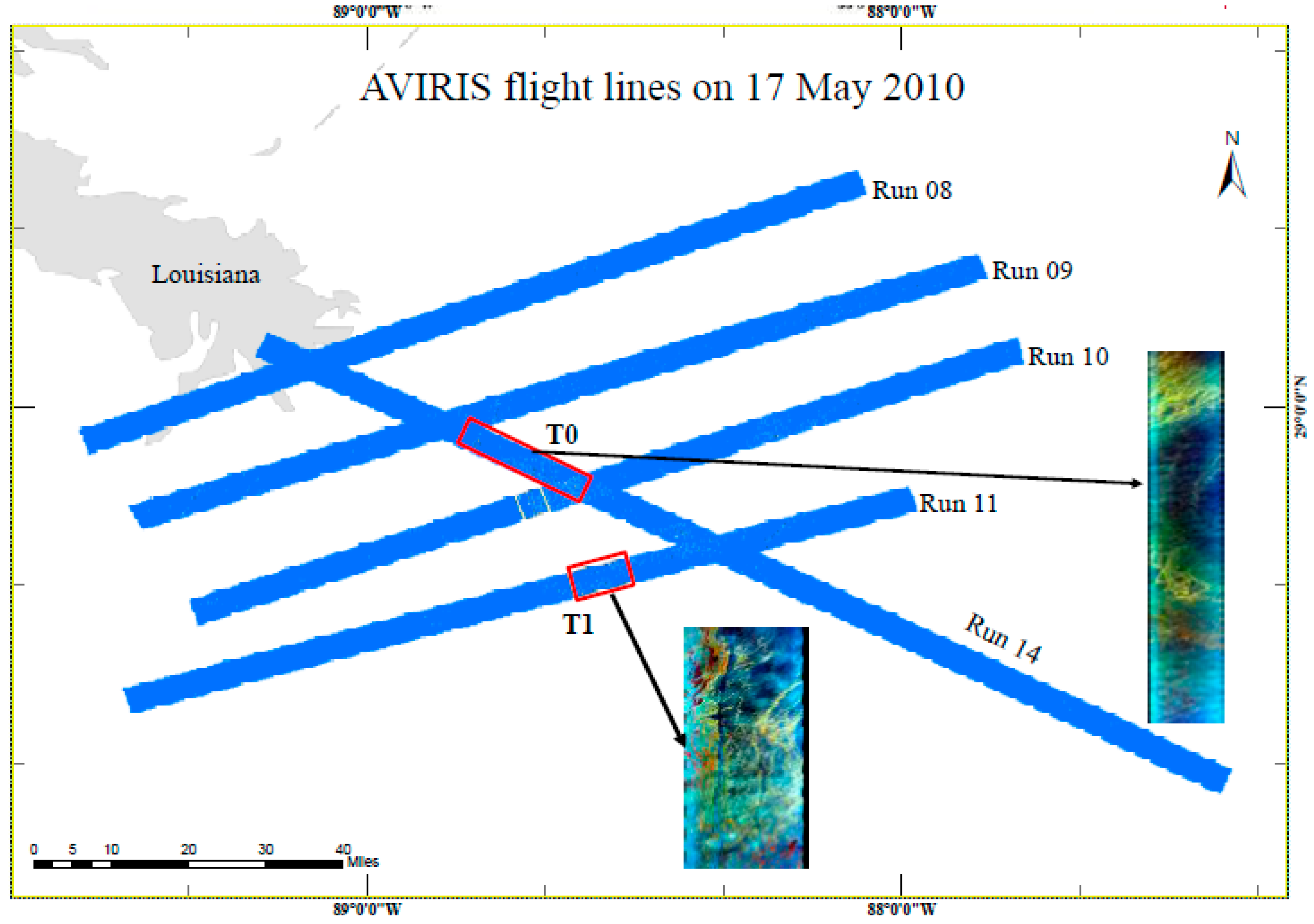
This paper focuses on the AVIRIS data, which was recorded with 224 bands in the 400 to 2500-nm wavelength range [32]. The flight names of the data are f100517t01p00r10 and f100517t01p00r11, and they have spatial resolutions of ~7.6 m and spectral resolution of 10 nm, respectively. The data was recorded on 17 May 2010 (Figure 1).
We collected training and test samples by human interpretation with reference to the Bonn Agreement [33], AVIRIS-derived oil volume maps [30], and spectral features [34]. The numbers of training and test samples were 469567 and 42676, respectively, which were selected from the image of Region T0 separately. These samples were divided into five classes (water, sheen, thin film, medium film, and thick film) (Table 1).
3. Methods
3.1. Overall Procedure
The overall workflow of this study is shown in Figure 2. First, three machine learning classifiers were implemented, which will be explained in detail later. Next, the training and test samples were prepared and read into each classifier separately. A series of parameters were used to train the model using the training samples. The 3-fold cross-validation was used to the training samples [35], which helped select the best combination of parameters. Each of the selected methods was tested using the test samples to calculate the accuracy. Finally, we adopted the best models of each classifier obtained previously to predict the label for each pixel and produce the oil slick distribution maps. We also compared the accuracy of the proposed method with the method in [23]. For the process of oil film distribution mapping, SIs and minimum redundancy maximum relevance (mRMR) were used to select the prominent features of each pixel in the image of T1 (Figure 1). The selected bands were loaded into the aforementioned classifiers.
3.2. Data Pre-Processing
Radiometric calibration and atmospheric correction, which will eliminate systematic errors introduced by system [36] and atmosphere, respectively, were applied to the hyperspectral raw data. While radiometric calibration is performed by the data provider, atmospheric correction is generally performed by the user. NASA/JPL had already processed the data to remove geometric errors introduced by the aircraft motion and radiation errors caused by the instruments. The atmospheric calibration was required to yield the surface reflectance values. The original values in the images were those of scaled radiance. Bands 1 to 110 have a scale factor of 300, bands 111 to 160 have a scale factor of 600, and bands 161 to 224 have a scale factor of 1200. Each band was divided by the corresponding scale factors, and a 16-bit integer radiation value was obtained in units of μW/(cm2 × sr × nm). Following this, the atmospheric correction was performed using the Fast Line-of-sight Atmospheric Analysis of Hypercubes (FLAASH) module in the ENVI software. In the FLAASH module, the atmospheric model parameters were tropical, and the aerosol model was maritime. After the atmospheric correction, the nearby pixels, which may contain oil film with similar thickness, have nearly identical spectra [37].
3.3. Feature Selection
Pal and Foody [38] showed that the classification accuracy is related to the dimension of the input features. The accuracy declines significantly with the addition of features, particularly if a small training data sample is used. However, Li et al. [39] found that the use of more bands improved classification accuracy. In this paper, we used images with and without band selection as inputs for the classifiers. The band selection methods we tested are based on the spectral index (SI) and mRMR measures.
(1) SI-based band selection
Zhao et al. [34] evaluated the usefulness of SIs to identify oil films with different thicknesses. They found that the spectral indices of hydrocarbons have a greater potential to detect oil slicks imaged with continuous true color. For sheens and seawater, seawater indices are more suitable. Among these indices, the Hydrocarbon Index (HI), Fluorescence Index (FI), and Rotation–Absorption Index (RAI) have been used to detect and characterize oil films of varying thicknesses [40,41] (Table 2). Other researchers [2,42,43] analyzed the spectral features of oil films with different thicknesses or area ratios and proposed useful spectral bands in the ranges of 507 to 670 nm, 756 to 771 nm, and 1627 to 1746 nm.
For the present work, we selected bands in the ranges of 490 to 885 nm and 1627 to 1746 nm.
(2) mRMR-based band selection
mRMR is an efficient feature selection algorithm proposed by Peng et al [44]. It penalizes a feature’s relevance by its redundancy in the presence of the other selected features. The relevance of a feature set and the redundancy of all features in the set are defined as follows:
where S is a feature set, C is the class, is the individual feature, and is the mutual information between feature and class C or features and is the relevance of S for the class C.
The mRMR of a feature set is obtained by simultaneously combining and into a single criterion function. Ding [45] defined the following two criteria to select the features: The MID: Mutual Information Difference criterion, and MIQ: Mutual Information Quotient criterion.
We used the MIQ, and 15 features were selected.
In hyperspectral data, the class label is an integer, but the bands are continuous. In order to use the algorithm, features are usually quantized to discretize the continuous bands into bins [46]. In this paper, the quantization boundary was set as , where and represent the estimated mean and standard deviation of the features, respectively.
3.4. Classifiers
(1) RF
Developed by Breiman in 2001, RF is one of the most commonly used machine learning ensembles. It trains a series of decision trees using randomized draws of training data. Following this, the entire forest of decision trees is used as a composite classifier. Data can be applied to the classifier once the forest is created. Furthermore, the prediction across each tree can be obtained [47].
A few parameters should be adjusted to make the RF classifier easier to use [48]. We used the RF classifier included in the Scikit-learn library [49]. The number of trees in the forest, the maximum number of features, and the minimum samples required to be present at a leaf node should be adjusted. The features are the reflectance bands in hyperspectral imagery. The maximum number of features is considered when looking for the best split. The number of trees used during this study was (10, 100, 500, 1000), among which the model with 100 trees got a relatively high accuracy and consumed a short amount of time. The maximum number of features is the square root of the number of features, and the minimum number of samples taken at each leaf is 1.
(2) SVM
SVM is a supervised learning model that uses learning algorithms to analyze and classify data. It is used widely owing to its effectiveness with small datasets [38]. A hyperplane is defined using the training data to classify in the SVM classifier [49,50]. For 2D data, the hyperplane is the line between two categories that separates the data most effectively. For high-dimensional classification, the data are mapped to space with a higher dimension, and the separator between categories becomes a plane. Hyper-parameters are used to dictate how the data is mapped onto the higher dimension. In this paper, the SVC model in the Scikit-learn library was used. The kernel support vector classifier that utilizes a one-vs.-one classification scheme, termed Radial Basis Function (RBF), was adopted. The kernel coefficient gamma for the RBF was set to (10−6, 0.01, 0.1, 0.2, 0.5). The penalty parameter C of the error term balances the misclassification of the training samples and the simplicity of the decision surface. A small C value makes a smooth decision surface, while a large C value implies that the model has greater freedom to select more samples as support vectors. We tested a series of C values, 1, 20, 70, 100, 200, 700, and 1000. The most suitable values found that kernel coefficient was 0.01 and C was 700.
(3) Convolutional Neural network
CNNs are feedforward neural networks whose artificial neurons can respond to a surrounding area of the covered part. CNNs comprise neurons with learnable weights and biases. Each neuron receives a line of inputs and performs dot product calculations. The output is the score for each category; the category with the highest score is used as the result. Typically, CNNs comprise four layers: Input, convolutional, pooling, and fully connected (FC). The output of the FC layer is the input to a simple linear classifier that generates the required classification result.
We used TensorFlow, a popular deep learning tool [51], to build our CNN. The architecture of the network comprises an input layer, a convolutional layer, a pooling layer, an FC neural network, and an FC Softmax layer that serves as the classifier. The flow diagram of our CNN process is shown in Figure 3.
The first layer of CNN is the input layer that contains the samples. To uniformly distribute the samples, a pre-processing procedure, such as normalization and dimensional reduction, could be performed. For this work, one-dimensional arrays, the spectra of all bands, and bands selected by mRMR and SI are used as the inputs.
The convolutional layer is the main part of CNN, and its parameters comprise a set of learnable filters [52]. Each filter is small but extends through the full depth of the input array. The outputs produced via convolving these filters across the input arrays are then fed into an active function. The outputs of convolutional layers are calculated using Equation (5).
where f is the active function, M and N are the width and height of the filter, respectively, and O(x,y) and w(x,y) are the value and weight of the xth row and yth column, respectively. b represents the bias.
In particular, for this work, two convolutional layers were utilized, the sizes and height of the filters were set as 3 and 1, respectively, and x was a constant (x = 1). We utilized the rectified linear unit (ReLU) as the active function. ReLU is an element-wise operation and replaces all negative pixel values in the feature map with zero. The purpose of ReLU is to introduce nonlinearity in the proposed convolutional net because most of the real-world data to be learned by the convolutional net would be non-linear.
The pooling layer can be regarded as a spectral subsampling or down-sampling of the convolutional features. It reduces the dimensionality of each feature but retrains the most important information. A max-pooling operation, which has been shown to work well in practice [11], was used in this paper. Through this operation, we defined a spectral neighborhood and took the largest element from the rectified feature within that window. For this work, the size of the window was 1 × 3.
The output of the pooling layer was then provided to the feature classification network, which comprised an FC neural network and an FC Softmax layer. The FC neural network contained a hidden layer with 128 notes. A 50% dropout level was adopted to randomly ignore nodes, which could prevent overfitting.
The output of the hidden layer was connected to the final classifier: a Softmax layer. This layer could produce a vector with the length that equals to the number of classes. Each value represents the probability that a feature belongs to a certain class. The Argmax function was adopted to find the location of the argument with the largest probability and finally provide a one-hot classification.
4. Results and Discussion
4.1. Feature Selection
The retention of important spectral features is essential. Hyperspectral remote sensing images can obtain nearly continuous spectra associated with the features. However, leaving too many spectral bands in the image will lead to redundancy between the bands, which will increase computational complexity without improving accuracy. Therefore, the hyperspectral remote sensing data are always dimensionally reduced. Band selection was used for dimension reduction. Using SIs-based method, 55 bands were selected and 15 bands remained after mRMR-based band selection. The computational complex was reduced dramatically, while the main spectral features were preserved. Images reduced with the mRMR indicator were less accurately classified than unreduced and SI-reduced images. This implies that mRMR band selection eliminated some useful features. The images reduced using the SIs indicator were reduced in dimension but lost no useful information [34]. This indicates that the thickness-related features of the images were part of the spectral information.
Band selection based on SIs and mRMR was applied to the original images, and the resulting bands were compared. Here, we named the original image as the all-bands image and the images after band selection as images of SIs selected bands and image mRMR selected bands.
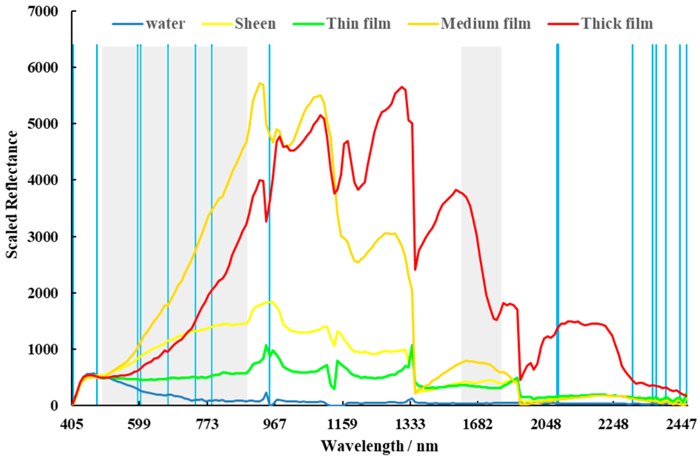
The dimensions of the data were reduced significantly through band selection (Figure 4). The selection results are mainly concentrated on the bands whose wavelength less than 970 nm or greater than 1600 nm. Using the mRMR method, 15 bands were selected for subsequent training and classification. The wavelengths of these bands are mainly concentrated in the range of 405 to 948 nm and 2357 to 2457 nm. According to the SIs, 55 bands that range from 490 to 880 nm to 1632 to 1742 nm were selected.
The separability between regions of interest (ROIs) is an important evaluation criterion for measuring the suitability of the training samples or ROIs. In the present study, the Jeffries–Matusita Distance (JMD) between various ROIs was calculated to evaluate the pair separation of the selected ROIs depending on the band selection method.
As shown in Table 3, the JMD values of the selected training samples from the all-band and band-selected images are between 1.89 and 2, which indicates that the selected samples were separable in all three cases [53]. The separation of the all-bands image was better than that of the band-selected images. The separability of the training samples is relatively low on the images after band selection through mRMR.
4.2. Accuracy Comparisons Among the Models
The sample distribution, overall accuracy (OA), producer’s accuracy (PA), and Kappa coefficient of the proposed and compared methods are listed in the Table 4. The accuracy was calculated based on the 42,676 test samples. By comparing the OAs of all the methods, we found that the methods with SIs selected bands received more accurate classification results than theses with all bands. Specifically, the proposed SIs+1D CNN had the best performance, while the All bands+RF performed the worst. We also calculated the accuracy of the method using Hu’s CNN [23]. The results of the method using Hu’s CNN were more accurate than those of SVM and RF, but less accurate than those of the proposed 1D CNN. This may be caused by the shallower architecture.
We calculated and listed the PA of each class using different methods. The PA of water is much higher than any other classes. This is because the spectra of water is obviously different from those of oil films (Figure 4 and Figure 5). Compared with the other models, the SIs+1D CNN had a much higher PA for water, sheen, and thick oil film. For the medium oil film, the method of All bands+SVM had the best classification result, while the SIs+1D CNN could mistakenly classify it as thick oil film. The thin films were easy to be categorized as sheen when the SIs+1D CNN is used.
During an oil spill emergency response, the most important thing is to distinguish the polluted and clean waters. Considering that, the SIs+1D CNN performs pretty well, because it can identify oil film accurately and classify the oil film thickness easily.
4.3. Running Time Comparisons Among the Models
The running time of each model is listed in Table 5. It was tested on the same running environment (Intel Core i5 CPU @ 2.64 GHz, use single core). The sample training time for RF and SVM refers to the time to fit the model to the training samples. The training time for proposed 1D CNN and Hu’s CN is the training time used to reach the highest OA. The sample validation time is the time used to predict labels for the test samples. The prediction time is the average time used to produce oil film distribution map for the hyperspectral image of region T1, including the time used for image input, output, and classification.
The model of All bands+RF took the longest training, validation, and prediction time. The method of mRMR+1D CNN took the shortest time for training, validation and, prediction. Generally, methods with Hu’s CNN needed less time than those with our CNN. This was mainly because Hu’s CNN had less layers, which meant it took less time to calculate and fit. Overall, The SIs+1D CNN model took relatively less prediction time, which is a very important factor for large scale oil spill extraction.
4.4. Case Studies
We selected one representative scene to compare the mapping results of each classifier. Figure 6 shows the AVIRIS true color image (color composite is R:638 nm, G:550 nm, B: 462 nm), the results obtained from All bands+1D CNN, SIs+1D CNN, mRMR+1D CNN, All bands+RF, SIs+RF, All bands+SVM, SIs+SVM, All bands+HU and SIs+HU for each scene. As can be seen in the images, most of the sea surface was clear water. In the area covered by the oil film, the oil film was mainly sheen and thin film. Thick oil films were scattered around the study area, which were labelled by the ellipses on the images. The medium oil films were distributed around the thick films.
By comparing the oil film distribution maps with the true color image, we found that the SIs+1D CNN, All bands +1D CNN, and SIs+SVM could identify most of the thick oil film. The model of SIs+1D CNN could precisely extract medium and thick oil film, while the other models consistently underestimated these two classes. The sheen oil film was mistakenly classified as water when the All bands+1D CNN, mRMR+1D CNN, RF, and Hu are used as the classifiers. The SIs+1D CNN could classify the sheen accurately (marked in red rectangle). Generally, the results obtained using SIs+1D CNN were substantially better than those from other models.
5. Conclusions and Future Work
In this paper, we proposed a band selection based 1D CNN method to perform oil film identification and thickness classification over AVIRIS hyperspectral images. We selected some bands with the main spectral features using spectral indices and mRMR. All models were trained and tested over the original all bands, SIs selected bands and mRMR selected bands separately. A cross-validation procedure was performed to find the best parameter combination for each method. All the selected models were tested over the test samples to calculate their OA, PA, and kappa coefficients, which demonstrated that the proposed SIs+1D CNN achieved an improvement in performance with respect to the rest of compared models in OA, and in PA for water, sheen, and thick oil film. The comparison of computation time was also made, and our proposed method reported that it needed relatively less prediction time. Moreover, all the mentioned methods were applied to an image to map the oil film distribution. It showed that our proposed method performed well in identification and classification of oil film.
In addition to the spectral information, the spatial context should also be considered during the oil film classification [37]. Normally, the thickness of oil film on sea surface changes gradually from sheen to thick. To improve classification performance, an intuitive idea is to design models using both spectral and spatial dimension, incorporating the spatial context into the 1D classifiers. Spatial information could provide additional discriminant information related to the effect of adjacent pixels, which could lead to more accurate classification maps [21]. Thus, 3D CNN should be considered in future studies.
Author Contributions
Conceptualization, Bingxin Liu; Data curation, Ying Li and Anling Liu; Formal analysis, Bingxin Liu; Project administration, Bingxin Liu; Writing—original draft, Bingxin Liu and Guannan Li.
Funding
This work was supported by the National Natural Science Foundation of China (Grant No. 51509030), Natural Science Foundation of Liaoning Province (Grant No. 20180550362), Dalian Innovation Support Foundation (Grand No. 2017RQ065), the Fundamental Research Funds for the Central Universities (Grant No. 3132014302) and China Scholarship Council.
Acknowledgments
The authors would like to thank JPL (https://aviris.jpl.nasa.gov/) for providing the data. We also thank Professor Jan-Peter Muller for giving some valuable advice.
Conflicts of Interest
The authors declare no conflict of interest.
References
- Fingas, M.; Brown, C. A Review of Oil Spill Remote Sensing. Sensors 2018, 18, 91. [Google Scholar] [CrossRef] [PubMed]
- Liu, B.; Li, Y.; Liu, C.; Xie, F.; Muller, J.-P. Hyperspectral Features of Oil-Polluted Sea Ice and the Response to the Contamination Area Fraction. Sensors 2018, 18, 234. [Google Scholar] [CrossRef] [PubMed]
- Cui, C.; Li, Y.; Liu, B.; Li, G. A new endmember preprocessing method for the hyperspectral unmixing of imagery containing marine oil spills. ISPRS Int. J. Geo-Inf. 2017, 6, 286. [Google Scholar] [CrossRef]
- Alves, T.M.; Kokinou, E.; Zodiatis, G.; Lardner, R. Deep-Sea Research II Hindcast, GIS and susceptibility modelling to assist oil spill clean-up and mitigation on the southern coast of Cyprus (Eastern Mediterranean). Deep Res. Part II 2015, 1980, 1–17. [Google Scholar] [CrossRef]
- Alves, T.M.; Kokinou, E.; Zodiatis, G. A three-step model to assess shoreline and offshore susceptibility to oil spills: The South Aegean (Crete) as an analogue for confined marine basins. Mar. Pollut. Bull. 2014. [Google Scholar] [CrossRef]
- Solberg, A.H.S.; Brekke, C.; Husøy, P.O. Oil spill detection in Radarsat and Envisat SAR images. IEEE Trans. Geosci. Remote Sens. 2007, 45, 746–754. [Google Scholar] [CrossRef]
- Fingas, M.; Brown, C. Review of oil spill remote sensing. Mar. Pollut. Bull. 2014, 83, 9–23. [Google Scholar] [CrossRef] [PubMed]
- Hughes, G.F. On the Mean Accuracy of Statistical Pattern Recognizerss. IEEE Trans. Inf. Theory 1968, 14, 55–63. [Google Scholar] [CrossRef]
- Paoletti, M.E.; Haut, J.M.; Plaza, J.; Plaza, A. A new deep convolutional neural network for fast hyperspectral image classification. ISPRS J. Photogramm. Remote Sens. 2017. [Google Scholar] [CrossRef]
- Khodadadzadeh, M.; Member, S.; Li, J.; Plaza, A.; Member, S. Spectral—Spatial Classification of Hyperspectral Data Using Local and Global Probabilities for Mixed Pixel Characterization. IEEE Trans. Geosci. Remote Sens. 2014, 52, 6298–6314. [Google Scholar] [CrossRef]
- Belgiu, M.; Drăgu, L. Random forest in remote sensing: A review of applications and future directions. ISPRS J. Photogramm. Remote Sens. 2016, 114, 24–31. [Google Scholar] [CrossRef]
- Guo, H.; Wu, D.; An, J. Discrimination of oil slicks and lookalikes in polarimetric SAR images using CNN. Sensors 2017, 17, 1837. [Google Scholar] [CrossRef]
- Guidici, D.; Clark, M. One-Dimensional Convolutional Neural Network Land-Cover Classification of Multi-Seasonal Hyperspectral Imagery in the San Francisco Bay Area, California. Remote Sens. 2017, 9, 629. [Google Scholar] [CrossRef]
- Makantasis, K.; Karantzalos, K.; Doulamis, A.; Doulamis, N. Deep supervised learning for hyperspectral data classification through convolutional neural networks. In Proceedings of the 2015 IEEE International Geoscience and Remote Sensing Symposium (IGARSS), Milan, Italy, 26–31 July 2015; pp. 4959–4962. [Google Scholar] [CrossRef]
- Liang, H.; Li, Q. Hyperspectral imagery classification using sparse representations of convolutional neural network features. Remote Sens. 2016, 8, 99. [Google Scholar] [CrossRef]
- Vetrivel, A.; Gerke, M.; Kerle, N.; Nex, F.; Vosselman, G. Disaster damage detection through synergistic use of deep learning and 3D point cloud features derived from very high resolution oblique aerial images, and multiple-kernel-learning. ISPRS J. Photogramm. Remote Sens. 2018. [Google Scholar] [CrossRef]
- Kussul, N.; Lavreniuk, M.; Skakun, S.; Shelestov, A. Deep Learning Classification of Land Cover and Crop Types Using Remote Sensing Data. IEEE Geosci. Remote Sens. Lett. 2017, 14, 778–782. [Google Scholar] [CrossRef]
- Chen, Y.; Jiang, H.; Li, C.; Jia, X.; Ghamisi, P. Deep feature sextraction and classification of hyperspectral images based on convolutional neural networks. IEEE Trans. Geosci. Remote Sens. 2016, 54, 6232–6251. [Google Scholar] [CrossRef]
- Li, Y.; Zhang, H.; Shen, Q. Spectral–spatial classification of hyperspectral imagery with 3D convolutional neural network. Remote Sens. 2017, 9, 67. [Google Scholar] [CrossRef]
- Chen, G.; Li, Y.; Sun, G.; Zhang, Y. Application of Deep Networks to Oil Spill Detection Using Polarimetric Synthetic Aperture Radar Images. Appl. Sci. 2017, 7, 968. [Google Scholar] [CrossRef]
- Fisher, P. The pixel: A snare and a delusion. Int. J. Remote Sens. 1997, 18, 679–685. [Google Scholar] [CrossRef]
- Zhang, L.; Zhang, L.; Kumar, V. Deep learning for Remote Sensing Data. IEEE Geosci. Remote Sens. Mag. 2016, 4, 22–40. [Google Scholar] [CrossRef]
- Ghamisi, P.; Plaza, J.; Chen, Y.; Li, J.; Plaza, A.J. Advanced Spectral Classifiers for Hyperspectral Images: A review. IEEE Geosci. Remote Sens. Mag. 2017, 5, 8–32. [Google Scholar] [CrossRef]
- Hu, W.; Huang, Y.; Wei, L.; Zhang, F.; Li, H. Deep convolutional neural networks for hyperspectral image classification. J. Sens. 2015, 2015, 258619. [Google Scholar] [CrossRef]
- Krizhevsky, A.; Sutskever, I.; Hinton, G.E. 1 ImageNet Classification with Deep Convolutional Neural Networks. Adv. Neural Inf. Process. Syst. 2012. [Google Scholar] [CrossRef]
- Mei, S.; Ji, J.; Hou, J.; Li, X.; Du, Q. Learning Sensor-Specific Spatial-Spectral Features of Hyperspectral Images via Convolutional Neural Networks. IEEE Trans. Geosci. Remote Sens. 2017, 55, 4520–4533. [Google Scholar] [CrossRef]
- Nieto-Hidalgo, M.; Gallego, A.J.; Gil, P.; Pertusa, A. Two-stage convolutional neural network for ship and spill detection using SLAR images. IEEE Trans. Geosci. Remote Sens. 2018, 56, 5217–5230. [Google Scholar] [CrossRef]
- Joye, S.B.; MacDonald, I.R.; Leifer, I.; Asper, V. Magnitude and oxidation potential of hydrocarbon gases released from the BP oil well blowout. Nat. Geosci. 2011, 4, 160–164. [Google Scholar] [CrossRef]
- Svejkovsky, J.; Lehr, W.; Muskat, J.; Graettinger, G.; Mullin, J. Operational utilization of aerial multispectral remote sensing during oil spill response: Lessons learned during the Deepwater Horizon (MC-252) spill. Photogramm. Eng. Remote Sens. 2012, 78, 1089–1102. [Google Scholar] [CrossRef]
- Leifer, I.; Lehr, W.J.; Simecek-Beatty, D.; Bradley, E.; Clark, R.; Dennison, P.; Hu, Y.; Matheson, S.; Jones, C.E.; Holt, B.; et al. State of the art satellite and airborne marine oil spill remote sensing: Application to the BP Deepwater Horizon oil spill. Remote Sens. Environ. 2012, 124, 185–209. [Google Scholar] [CrossRef] [Green Version]
- Clark, B.R.N.; Swayze, G.A.; Leifer, I.; Livo, K.E.; Kokaly, R.; Hoefen, T.; Lundeen, S.; Eastwood, M.; Green, R.O.; Pearson, N.; et al. A Method for Quantitative Mapping of Thick Oil Spills Using Imaging Spectroscopy; US Geological Survey: Tucson, AZ, USA, 2010.
- Liu, B.; Li, Y.; Chen, P.; Zhu, X. Extraction of Oil Spill Information Using Decision Tree Based Minimum Noise Fraction Transform. J. Indian Soc. Remote Sens. 2016, 44. [Google Scholar] [CrossRef]
- Green, R.O.; Eastwood, M.L.; Sarture, C.M.; Chrien, T.G.; Aronsson, M.; Chippendale, B.J.; Faust, J.A.; Pavri, B.E.; Chovit, C.J.; Solis, M. Imaging spectroscopy and the airborne visible/infrared imaging spectrometer (AVIRIS). Remote Sens. Environ. 1998, 65, 227–248. [Google Scholar] [CrossRef]
- Bonn Agreement. Bonn Agreement Aerial Operations Handbook; Bonn Agreement Secretariat: London, UK, 2017. [Google Scholar]
- Zhao, D.; Cheng, X.; Zhang, H.; Niu, Y.; Qi, Y. Evaluation of the Ability of Spectral Indices of Hydrocarbons and Seawater for Identifying Oil Slicks Utilizing Hyperspectral Images. Remote Sens. 2018, 10, 421. [Google Scholar] [CrossRef]
- Carranza-García, M.; García-Gutiérrez, J.; Riquelme, J. A Framework for Evaluating Land Use and Land Cover Classification Using Convolutional Neural Networks. Remote Sens. 2019, 11, 274. [Google Scholar] [CrossRef]
- Alparone, L.; Selva, M.; Aiazzi, B.; Baronti, S.; Butera, F.; Chiarantini, L. Signal-dependent noise modelling and estimation of new-generation imaging spectrometers. In Proceedings of the WHISPERS ’09—1st Workshop on Hyperspectral Image and Signal Processing: Evolution in Remote Sensing, Grenoble, France, 26–28 August 2009; pp. 1–4. [Google Scholar]
- Acquarelli, J.; Marchiori, E.; Buydens, L.M.C.; Tran, T.; van Laarhoven, T. Spectral-spatial classification of hyperspectral images: Three tricks and a new learning setting. Remote Sens. 2018, 10, 1156. [Google Scholar] [CrossRef]
- Pal, M.; Foody, G.M. Feature selection for classification of hyperspectral data by SVM. IEEE Trans. Geosci. Remote Sens. 2010, 48, 2297–2307. [Google Scholar] [CrossRef]
- Loos, E.; Brown, L.; Borstad, G.; Mudge, T.; Álvarez, M. Characterization of Oil Slicks at Sea Using Remote Sensing Techniques. In Proceedings of the OCEANS, Yeosu, Korea, 21–24 May 2012. [Google Scholar]
- Kühn, F.; Oppermann, K.; Hörig, B. Hydrocarbon index—An algorithm for hyperspectral detection of hydrocarbons. Int. J. Remote Sens. 2004, 25, 2467–2473. [Google Scholar] [CrossRef]
- Lu, Y.; Tian, Q.; Qi, X.; Wang, J.; Wang, X. Spectral response analysis of offshore thin oil slicks. Spectrosc. Spectr. Anal. 2009, 29, 986–989. [Google Scholar]
- Liu, B.; Li, Y.; Zhang, Q.; Han, L. Assessing Sensitivity of Hyperspectral Sensor to Detect Oils with Sea Ice. J. Spectrosc. 2016, 2016, 1–9. [Google Scholar] [CrossRef]
- Peng, H.; Long, F.; Ding, C. Feature selection based on mutual information: Criteria of Max-Dependency, Max-Relevance, and Min-Redundancy. IEEE Trans. Pattern Anal. Mach. Intell. 2005, 27, 1226–1238. [Google Scholar] [CrossRef] [PubMed]
- Ding, C.; Peng, H. Minimum Redundancy Feature Selection from Microarray Gene Expression Data. J. Bioinform. Comput. Biol. 2005, 3, 523–528. [Google Scholar] [CrossRef]
- Su, J.; Yi, D.; Liu, C.; Guo, L.; Chen, W.H. Dimension reduction aided hyperspectral image classification with a small-sized training dataset: Experimental comparisons. Sensors (Switzerland) 2017, 17, 2726. [Google Scholar] [CrossRef] [PubMed]
- Breiman, L. Random Forests. Mach. Learn. 2001, 45, 5–32. [Google Scholar] [CrossRef] [Green Version]
- Zhao, C.; Wan, X.; Zhao, G.; Yan, Y. Spectral–spatial classification of hyperspectral images using trilateral filter and stacked sparse autoencoder. J. Appl. Remote Sens. 2017, 11, 016033. [Google Scholar] [CrossRef]
- Pedregosa, F.; Weiss, R.; Brucher, M. Scikit-learn Machine Learning in Python. J. Mach. Learn. Res. 2011, 12, 2825–2830. [Google Scholar] [CrossRef]
- Zhao, W.; Du, S. Spectral-Spatial Feature Extraction for Hyperspectral Image Classification: A Dimension Reduction and Deep Learning Approach. IEEE Trans. Geosci. Remote Sens. 2016, 54, 4544–4554. [Google Scholar] [CrossRef]
- Ball, J.E.; Anderson, D.T.; Chan, C.S. A Comprehensive Survey of Deep Learning in Remote Sensing: Theories, Tools and Challenges for the Community. J. Appl. Remote Sens. 2017, 11, 042609. [Google Scholar] [CrossRef]
- Ammour, N.; Alhichri, H.; Bazi, Y.; Benjdira, B.; Alajlan, N.; Zuair, M. Deep learning approach for car detection in UAV imagery. Remote Sens. 2017, 9, 312. [Google Scholar] [CrossRef]
- Fukunaga, K. Introduction to Statistical Pattern Recognition, 2nd ed.; Academic Press: New York, NY, USA, 1990. [Google Scholar]
Figure 1.
AVIRIS flight lines covered on 17 May 2010. The models were trained and tested using image of T0, and applied to images of regions T1.
Figure 1.
AVIRIS flight lines covered on 17 May 2010. The models were trained and tested using image of T0, and applied to images of regions T1.

Figure 2.
The overall flowchart for all methods described in this study.

Figure 3.
Flow chart of the proposed convolutional neural network (CNN).

Figure 4.
Band selection results. The bands covered by grey areas were selected by mRMR. The blue lines indicate bands selected according to the SIs.
Figure 4.
Band selection results. The bands covered by grey areas were selected by mRMR. The blue lines indicate bands selected according to the SIs.

Figure 5.
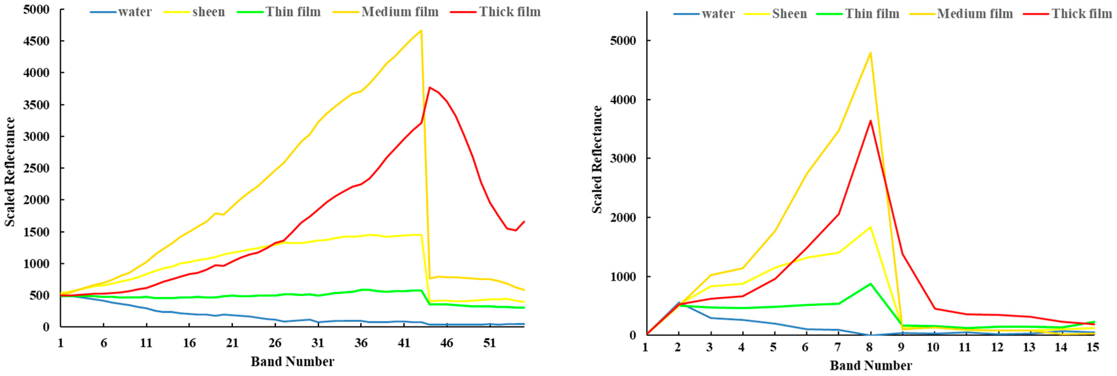
Spectra with band number of images after band selection. Left: SIs-based selected bands; Right: mRMR-based selected bands.
Figure 5.
Spectra with band number of images after band selection. Left: SIs-based selected bands; Right: mRMR-based selected bands.

Figure 6.
Classification results of Region T2. (a) composed true color image (R: 638 nm, G: 550 nm, B: 462 nm), result images using (b) All bands+1D CNN, (c) SIs+1D CNN, (d) mRMR+1D CNN, (e) All bands+RF, (f)SIs+RF, (g) All bands+SVM, (h) SIs+SVM, (i) All bands+HU, and (j) SIs+HU.
Figure 6.
Classification results of Region T2. (a) composed true color image (R: 638 nm, G: 550 nm, B: 462 nm), result images using (b) All bands+1D CNN, (c) SIs+1D CNN, (d) mRMR+1D CNN, (e) All bands+RF, (f)SIs+RF, (g) All bands+SVM, (h) SIs+SVM, (i) All bands+HU, and (j) SIs+HU.


Table 1.
Oil film description and thickness according to the Bonn Agreement and in this study.
| Bonn Agreement Classes | This Study | |||
|---|---|---|---|---|
| Code | Description/Appearance | Layer Thickness/μm | Class | Layer Thickness/μm |
| 1 | 0 (sea water) | |||
| 1 | Sheen | 0.04–0.3 | ||
| 2 | Rainbow | 0.3–5.0 | ||
| 3 | Metallic | 5.0–50 | 2 | <50 (sheen) |
| 4 | Discontinuous true color | 50–200 | 3 | 50–100 (thin film) |
| 4 | 100–200 (medium film) | |||
| 5 | Continuous true color | >200 | 5 | >200 (thick film) |
Table 3.
Pair separation between each training sample in terms of the Jeffries–Matusita distance (JMD).
Table 3.
Pair separation between each training sample in terms of the Jeffries–Matusita distance (JMD).
| Water | Sheen | Thin | Medium | Thick | ||
|---|---|---|---|---|---|---|
| All Bands | Water | / | 2.00000 | 2.00000 | 2.00000 | 2.00000 |
| Sheen | 2.00000 | / | 1.99977 | 2.00000 | 2.00000 | |
| Thin | 2.00000 | 1.99977 | / | 2.00000 | 2.00000 | |
| Medium | 2.00000 | 2.00000 | 2.00000 | / | 1.99996 | |
| Thick | 2.00000 | 2.00000 | 2.00000 | 1.99996 | / | |
| SIs Selected Bands | Water | / | 2.00000 | 2.00000 | 2.00000 | 2.00000 |
| Sheen | 2.00000 | / | 1.99778 | 2.00000 | 2.00000 | |
| Thin | 2.00000 | 1.99778 | / | 1.99891 | 2.00000 | |
| Medium | 2.00000 | 2.00000 | 1.99891 | / | 1.99996 | |
| Thick | 2.00000 | 2.00000 | 2.00000 | 1.99996 | / | |
| mRMR Selected Bands | Water | / | 1.99506 | 1.99757 | 2.00000 | 2.00000 |
| Sheen | 1.99506 | / | 1.89845 | 1.99747 | 1.99964 | |
| Thin | 1.99757 | 1.89845 | / | 1.99999 | 1.99814 | |
| Medium | 2.00000 | 1.99747 | 1.99999 | / | 1.97672 | |
| Thick | 2.00000 | 1.99964 | 1.99814 | 1.97672 | / |
Table 4.
Test samples distribution and testing results.
| Sample Distribution | Class | Water | Sheen | Thin Film | Medium Film | Thick Film | OA | Kappa |
|---|---|---|---|---|---|---|---|---|
| Samples | 32405 | 7443 | 2343 | 274 | 211 | |||
| PA | All bands+1D CNN | 89.62% | 60.43% | 61.70% | 59.12% | 57.08% | 82.62% | 0.5732 |
| SIs+1D CNN | 90.43% | 65.42% | 68.01% | 63.14% | 72.99% | 84.57% | 0.6259 | |
| mRMR+1D CNN | 88.88% | 61.91% | 68.09% | 62.41% | 52.61% | 82.68% | 0.5796 | |
| All bands+RF | 87.18% | 52.16% | 70.76% | 62.04% | 56.40% | 79.86% | 0.5095 | |
| SIs+RF | 86.13% | 57.01% | 77.80% | 64.60% | 59.24% | 80.31% | 0.5169 | |
| All bands+SVM | 86.83% | 57.14% | 66.41% | 70.44% | 67.30% | 80.33% | 0.5345 | |
| SIs+SVM | 89.94% | 42.34% | 81.65% | 54.74% | 69.19% | 80.86% | 0.5221 | |
| All bands+HU | 88.09% | 63.12% | 73.58% | 54.74% | 63.03% | 82.60% | 0.5832 | |
| SIs+HU | 89.11% | 64.21% | 72.86% | 43.43% | 62.56% | 83.45% | 0.5996 |
Table 5.
Running time comparison (averaged from 20 repeated experiments).
| Sample Training Time/min | Sample Validation Time/min | Prediction Time/min | |
|---|---|---|---|
| All bands+1D CNN | 15.816 ± 0.150 | 2.761 ± 0.011 | 5.732 ± 0.023 |
| SIs+1D CNN | 7.452 ± 0.071 | 2.012 ± 0.010 | 3.893 ± 0.021 |
| mRMR+1D CNN | 4.468 ± 0.053 | 1.732 ± 0.004 | 2.892 ± 0.022 |
| All bands+RF | 19.238 ± 0.127 | 3.401 ± 0.019 | 7.642 ± 0.018 |
| SIs+RF | 6.919 ± 0.029 | 2.174 ± 0.017 | 5.964 ± 0.011 |
| All bands+SVM | 12.174 ± 0.272 | 2.417 ± 0.034 | 4.724 ± 0.009 |
| SIs+SVM | 6.102 ± 0.077 | 1.936 ± 0.018 | 3.368 ± 0.026 |
| All bands+HU | 13.112 ± 0.217 | 2.382 ± 0.082 | 4.836 ± 0.013 |
| SIs+HU | 5.766 ± 0.026 | 1.103 ± 0.004 | 3.062 ± 0.028 |
© 2019 by the authors. Licensee MDPI, Basel, Switzerland. This article is an open access article distributed under the terms and conditions of the Creative Commons Attribution (CC BY) license (http://creativecommons.org/licenses/by/4.0/).
Share and Cite
MDPI and ACS Style
Liu, B.; Li, Y.; Li, G.; Liu, A. A Spectral Feature Based Convolutional Neural Network for Classification of Sea Surface Oil Spill. ISPRS Int. J. Geo-Inf. 2019, 8, 160. https://doi.org/10.3390/ijgi8040160
AMA Style
Liu B, Li Y, Li G, Liu A. A Spectral Feature Based Convolutional Neural Network for Classification of Sea Surface Oil Spill. ISPRS International Journal of Geo-Information. 2019; 8(4):160. https://doi.org/10.3390/ijgi8040160
Chicago/Turabian StyleLiu, Bingxin, Ying Li, Guannan Li, and Anling Liu. 2019. "A Spectral Feature Based Convolutional Neural Network for Classification of Sea Surface Oil Spill" ISPRS International Journal of Geo-Information 8, no. 4: 160. https://doi.org/10.3390/ijgi8040160
Note that from the first issue of 2016, this journal uses article numbers instead of page numbers. See further details here.