SLiX: A GIS Toolbox to Support Along-Stream Knickzones Detection through the Computation and Mapping of the Stream Length-Gradient (SL) Index

Abstract

The stream length-gradient (SL) index is widely used in geomorphological studies aimed at detecting knickzones, which are extensive along-stream deviations from the typical concave-up shape assumed for stream longitudinal profiles at steady-state conditions. In particular, SL was practical for identifying anomalous gradients along bedrock stream channels in mountainous catchments. This work presents the GIS toolbox SLiX designed to extract values of the SL index, starting from Digital Elevation Models (DEMs). SLiX is also suitable for the spatial analysis of the SL values, allowing for the identification of landscape portions where anomalous high values of SL occur and, consequently, those catchment sectors where stream channels show peaks in the erosional dynamic. The SLiX main outputs are (i) point shapefiles containing, among stream channels attributes, the extracted values of SL along the stream network analyzed, and (ii) SL anomaly maps in GeoTIFF format, computed through the Hotspot and Cluster Analysis (HCA), that permit the detection of the catchment sectors where the major SL anomalies occur and consequently the principal knickzones. The application of the proposed tool within an experimental catchment located in the Northern Apennines of Italy demonstrated the proper functionality and the potential of its use for different geomorphological and environmental studies. The accurate and cost-effective detection of anomalous changes in stream gradient ensured by SLiX is of great interest and can be useful for studies aimed at unravelling the Earth processes responsible of their formation (e.g., active hillslope processes, such as landslides directly interacting with the streambed, presence of geological structures, and meander cut-off). The applications of SLiX have clear implications for preliminary analyses, at a regional scale in different morpho-climatic contexts, for the hydrological management of river basins and/or to prevent geological hazards related to the fluvial erosional dynamics.

1. Introduction

The landscape evolution, due to the opposing actions of active tectonic uplift and subsidence, as well as erosion and sedimentation processes, implies steady changes of Earth surface topography [1]. The geometry and spatial distribution of drainage networks can reflect the style and timing of the landscape evolution at different scales, from catchments to mountain ranges. The geomorphometry of stream longitudinal profiles has been helpful so far for modeling the evolution of erosional landscapes [2] and reference therein] and, in particular, for better understanding the role of different superimposed factors, such as those derived from active tectonics and climate change [3].

Many geomorphic indices have been proposed to unravel the topographic fingerprints of surface and subsurface processes [2] and reference therein]. Among these, the stream length-gradient (SL) index [4] allows to highlight deviations from the concave-up shape of river longitudinal profiles and to mark knickpoints/knickzones where the stream gradient show anomalous values [5].

The form of a bedrock stream long-profile at steady-state conditions, according to Hack (1973) [4], can be described by the equation as follows:

H = C − K * logL,

(1)

where H is the altitude of a given point along the stream channel and L is the distance of the point far from the channel initiation. A stream long-profile at steady-state conditions has typically the form of a straight line on the H-logL space (i.e., Hack’s profile); therefore, deviations from steady-state conditions can be easily revealed by the variations of the angular coefficient K of Equation (1).

If derived on the distance, L, Equation (1) becomes the following:

K (SL) = dH/dL * L,

(2)

where K is the stream length-gradient (SL) index (from here on simply SL) [4]. The apparent facility of the index calculation and, in most recent time, the possibility to use high-resolution digital elevation data and geo-information technologies (i.e., GIS software, above all), made the SL one of the most used in geomorphological studies among a range of indexes [5,6] and reference therein, especially on those studies finalized to recognize the effects of active tectonics on drainage network [2] and reference therein. Therefore, even if not the unique method (e.g., [7]), SL is a proper tool, providing an easy way to find anomalous gradients along stream long-profiles at a range of scale, i.e., knickpoints and knickzones [8].

Knickzones can be produced by local or regional variations of erosional base-level [9,10]. The latter can be due to a variety of factors and processes: (i) geological structures (i.e., faults) either active or not; (ii) differential erosion due to litho-structural changes; (iii) landslides directly interacting with the streambed; (iv) stream piracy and meander cut-off; and (v) anthropogenic features. Therefore, the appropriate geological and morphogenetic interpretation of the recognized SL anomalies is fundamental [6,8].

The growing availability of geo-information technologies allows facing geomorphological issues with new tools. In particular, the application of geomorphometric indices for investigating the interplay between different geological and geomorphological factors and processes in shaping the landscape can take advantage from GIS tools [11].

A step-by-step procedure consisting of several phases for extracting and validating SL values from Digital Elevation Models (DEMs) has been proposed in Troiani et al. (2014) [6]. These authors also proposed a complete geostatistical procedure for fine-tuning the spatial analysis of the index values and for selecting the proper stream-segmentation method that can highly affect the computation accuracy of the SL index values.

Subsequently, Troiani et al. (2017) [8] proposed a new mapping method of SL, applicable at both small catchment and regional scale, based on the Getis–Ord statistic (i.e., SL-HCA maps), useful for identifying and fine-tuning the interpretation of wide stream reaches affected by anomalous high gradients (i.e., knickzones).

In this work, the development of the open-source toolbox named SLiX is presented and discussed. SLiX works in ArcGIS 10.6 and allows users to extract SL values starting from DEM and producing, as a final output, both SL dot-maps and SL-HCA maps (sensu [8]), highlighting the main SL anomalies within the analyzed catchments. The proposed tool is helpful for supporting the detection of knickzones in different geological contexts and for inferring their morphogenetic implications.

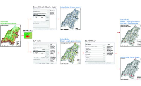
2. Principles of Design and Processing Tools

SLiX is designed for the automatic extraction of SL values, starting from different DEM sources, and for the spatial analysis of SL values within a given area, at different scales, from catchment to mountain range.

The SL index is calculated, for a given reach along a given channel, using the Equation (2) (Figure 1).

The complete GIS procedure requires first the stream network extraction, then the calculation of SL values, and finally the adequate classification of computed SL values, to highlight the zones with anomalous high values. The entire step-by-step procedure, which requires about 15 different actions, is replicable, by means of different tools in a Geographical Information System (GIS) software (e.g., Q-GIS and ArcGis), eventually supported by external packages (e.g., ArcHydroTools and ETGeowizard), performing in a systematic order each single step.

2.1. Stream Network Extraction

The procedure for the extraction of SL values requires as a first step the drainage network delineation from a DEM dataset. In order to guarantee the hydrological correctness, an operation of filling sinks and removing peaks, possibly due to the original elevation data inaccuracy or to interpolation errors, is required [12]. The successive step includes the Flow Direction raster calculation using a single-flow algorithm (i.e., D8) and, subsequently, the Flow Accumulation raster extraction. The first parameter determines the direction of flow for each raster cell, while the second one estimates, for each raster cell, the cumulated upstream contributing area [13,14,15]. The SL is valid only for bedrock streams and its use is therefore limited to mountainous catchment sectors and/or within sectors along stream channels where erosional morphodynamics predominates. In these geomorphological conditions, the D8 single flow algorithm revealed the best choice [16] and reference therein.

The Flow Accumulation raster has to be binary codified into “Channel” and “Not-Channel”, in order to outline properly the channels network. Therefore, it is fundamental to ensure the extraction of a “real” channels network, including only the landscape portions experiencing fluvial process [17,18]. This can be ensured by determining an appropriate value for the channel initiation in terms of the contributing area, which can be selected detecting the critical threshold separating slope and fluvial process domains in the relationship between drainage area and slope [16,17,18].

2.2. SLIndex Calculation

The extracted channels network has to be segmented in regular distributed reaches in order to allow the calculation of the SL values along reaches having either the same length or the same altitude range. This computation is affected by the stream segmentation method, which can plan channel reaches with fixed dH or fixed dL (cfr. Equation (2)) [4,5,6]. Considering the calculation adopting channel reaches with fixed dL [6], for each channel reach of the obtained dataset, the variation of elevation (dH) and the distance from the channel initiation point (L) can be then computed. The choice to use a fixed dL is based on the results obtained in previous comparative analyses, which considered different segmentation methods [6]. This approach also allows for a constant point spacing and avoids an irregular distribution of SL values [5]. The elevation values are extracted directly from the input DEM dataset, adding to each channel reach the z-values. The variation of elevation (dH) is computed as subtraction between the maximum and minimum values along each channel reach, the latter being successively converted in single point (i.e., midpoint of the considered reach). The channel length is extracted from the Flow Length raster dataset, derived from the input DEM, exploiting the previously derived Flow Direction and Flow Accumulation raster datasets. The Flow Length data provides, in fact, the upstream distance along a channel, hence the L value (cfr. Equation (2)) for each point of the dataset. At this step, having at disposal all the parameters included Equation (2), it is now possible to calculate the SL value for each point of the dataset.

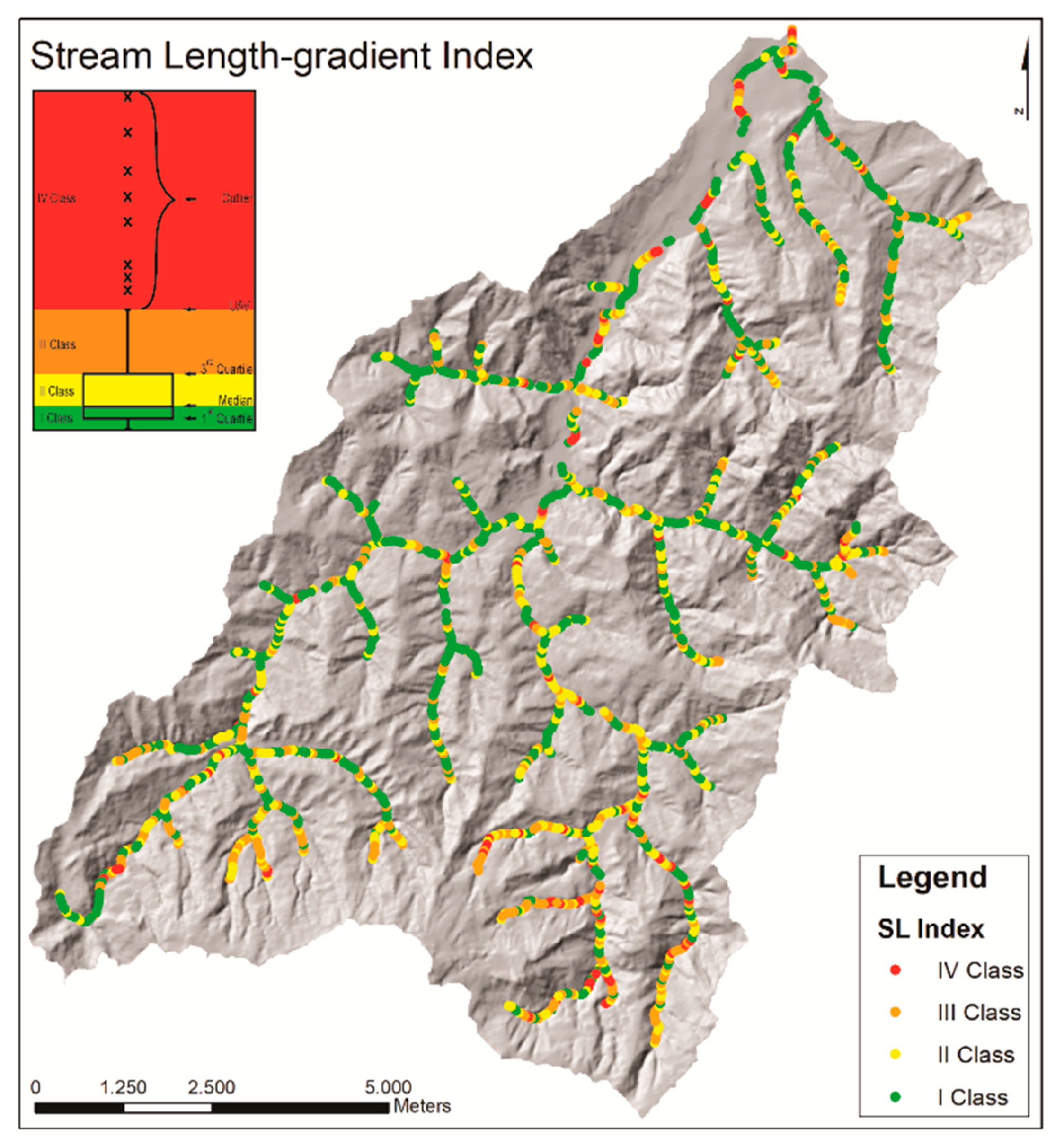
2.3. SL Values Classification and Interpretation

The SL values can now be used for proper outcomes symbology and/or for successive spatial analysis, e.g., using Ordinary Kriging [5,6,19,20] or the Hotspot and Cluster analysis [8], which are helpful to estimate landscape sectors where the parameters are anomalously high. In particular, the Hotspot and Cluster Analysis (HCA) has been proven a suitable method for the geo-spatial visualization of SL index values because it helps to objectively select the zones with anomalous high values. Indeed, this approach, based on the Getis–Ord Gi*statistic, allows the identification of knickzones on the stream profiles, measuring the clustering of highest SL values compared within the entire dataset of the analyzed river basin [8].

2.4. SLiX Toolbox

The step-by-step procedure described in the previous sections is summarized in the SLiX Toolbox. This Toolbox includes three different models: (i) the Stream Network Extraction (SNE), (ii) the SLiX model; and (iii) the Stream Length-Gradient index Hotspot and Cluster Analysis (SL-HCA). The developed models, featured exploiting the ArcGis Model Builder visual programming language, allow to automatically deriving the drainage network and SL values starting from DEM, as well as the SL hotspots and correlated kernel density starting from SL values. In particular, the SLiX model summarizes with a single input mask and only one output shapefile the entire procedure of SL index calculation (Figure 2 and Figure 3).

The schematic workflow for the SLiX model is presented in Figure 2.

The Stream Network Extraction model provides, as intermediate output, an independent delineation of the drainage network in vector format (Figure 3). The latter can be useful for further or other geomorphological and geomorphometric analyses.

The output of SLiX model (SL point values) appears, at a first glance, unclassified. According to different statistical classification criteria, the suggested classification to apply considers the quartile distribution and allows for the subdivision of the results into four classes (Figure 4), respectively: (i) 0—median value; (ii) median value—third quartile; (iii) third quartile—Upper Adjacent Value (UAV); and (iv) outlier values [6,8,20].

For contributing to the interpretation of the SL anomalies using the Stream Length-Gradient Hot Spot and Cluster Analyses (SL-HCA) proposed by Troiani et al. (2017) [8], the SL-HCA model has been finally introduced in the SLiX Toolbox (Figure 5). This model provides two outputs: (1) the point shapefile of the SL-HCA, using the Getis–Ord algorithm showing SL cold and hotspot spatial distribution; (2) kernel density raster map with the associated statistics table. The first output allows showing the distribution of the zones along the drainage network with the clustering of SL index values anomalous high. The second is a derived map, which helps to visualize major anomalous zones, being a more straightforward product (Figure 5).

3. Example of Application

The proposed toolbox has been tested with real data in several basins and the application in the Apsa River catchment, a right tributary of the Foglia River in the Northern Apennines is here presented (Figure 6).

The area revealed an excellent site to test the functionality and reliability of SLiX toolbox because of the complex litho-structural setting representative of active landscapes carved on uplifting, lithological complex fold-and-thrust belts. The Apsa River catchment is also one of those affected by active and dormant large landslides affecting hillslopes characterized by both hard and soft lithotypes and active fluvial morphogenesis generating both erosional and depositional morphotypes.

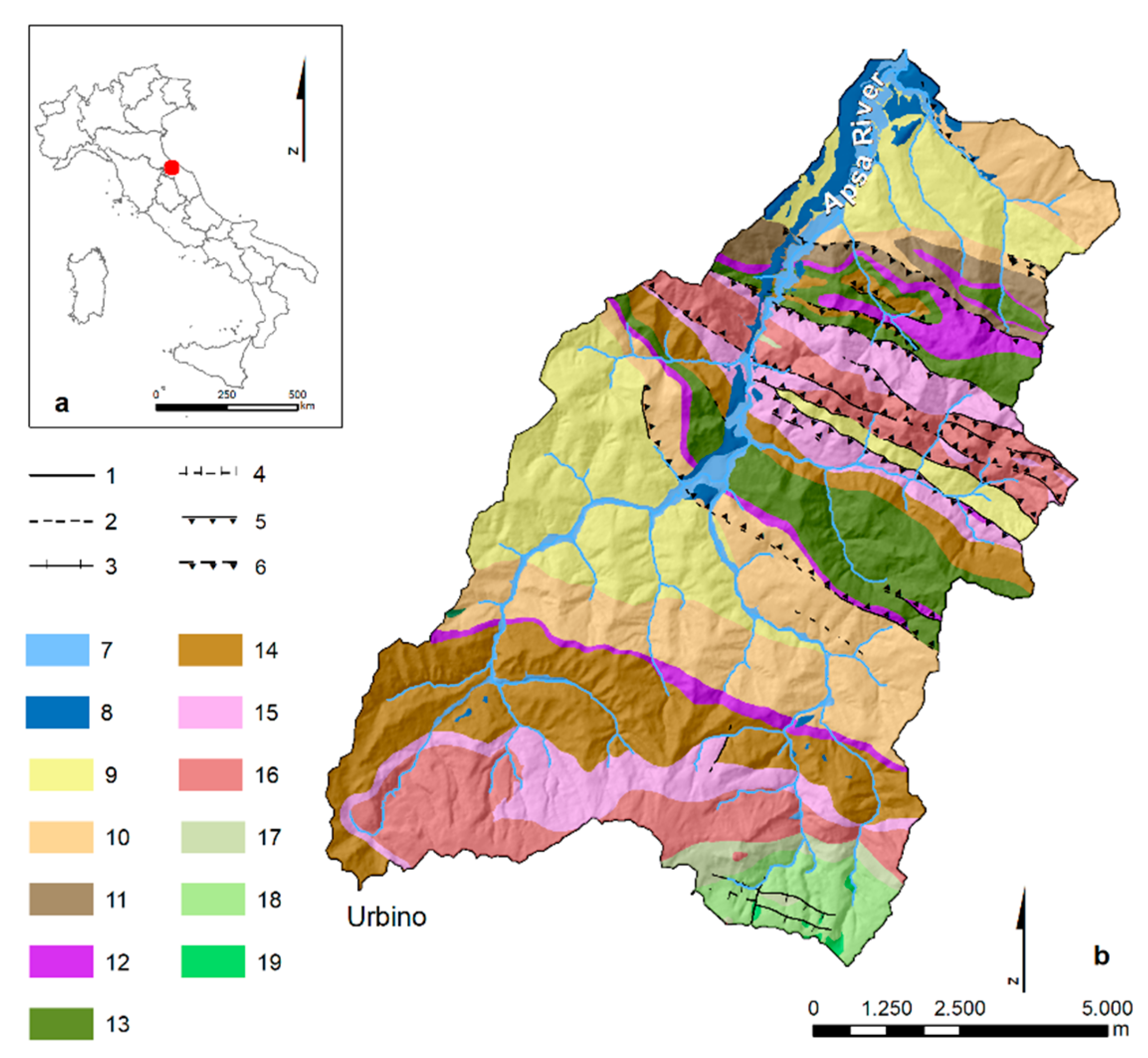
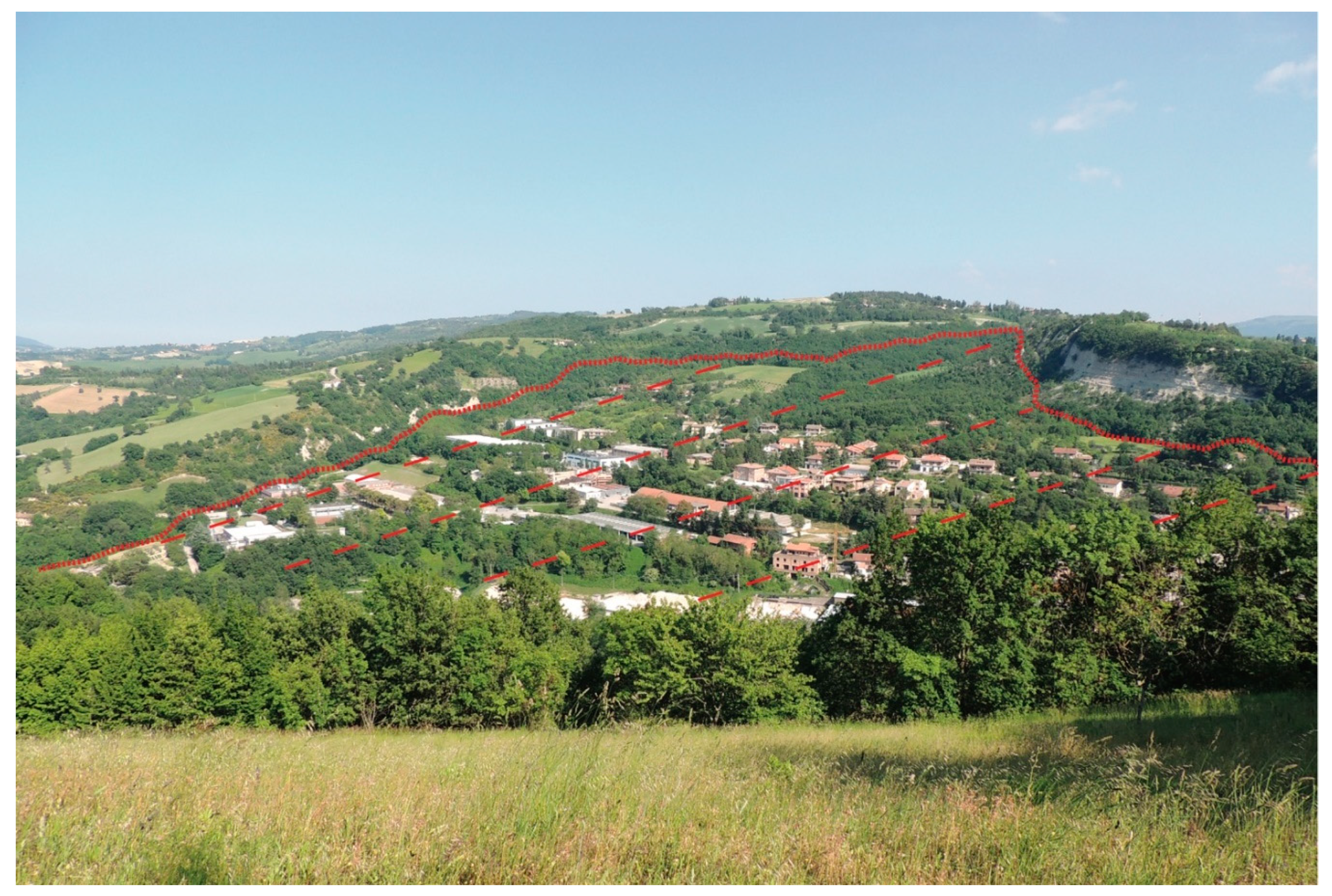
3.1. General Setting

The Apsa River catchment extents for about 100 km² in the piedmont, hilly sector of the northern portion of the Marche Apennines in central Italy. Elevations range from about 40 m, at the Apsa outlet, up to 640 m a.s.l., in the surroundings of the relief called Colla Romana in the southern portion of the catchment (Figure 6).

The bedrock generally consists of a multilayer terrigenous stratigraphic succession belonging to the Meso-Cenozoic Umbria-Marche stratigraphic sequence [21,22,23], principally composed by an irregular alternation of arenites, pelites, marly-limestones and limestones [23]. In this sector of the Apennines, Messinian evaporites and diatomitic levels also outcrop (Figure 6). The main geological structures, represented by a rhythmic succession of anticline and syncline folded structures and thrust faults, generally strike in NW–SE and WNW–ESE directions.

The outcropping lithologies and their structural attitude favor the presence of earth-flows and earth-slides of different sizes and state of activity that are widespread in the whole area, in particular where the most erodible marls and pelites outcrop [24]. Rockslides and deep-seated gravitational slope deformations (DSGSDs) have been also identified in the study area [25,26,27] and in the surrounding region [28,29].

The drainage network is in general characterized by bedrock channels that are mostly entrenched in incised V-shaped valley that generally flow cross-cutting the main geological structures. Valley sectors entrenched in the most erodible marly and pelitic lithologies are in general more gently shaped. Valley entrenchment is principally due to Quaternary tectonic uplift that have affected this sector of the Apennines [30]. The hillslope-channel system along the tributary catchments is in general well connected; in particular, hillslopes are separated from streambeds by a fluvial plain never exceeding the width of 5–10 m. On the contrary, along the Apsa trunk stream the hillslope-channel system is disconnected and a fluvial plain characterized by a width > 10–20 m occurs, especially along the downstream sectors.

3.2. SL Values Extraction and Anomaly Map Calculation

The SLiX test at the Apsa River catchment based on a regular grid DEM with a cell-size of 10 m, which has been derived by using the ANUDEM algorithm from the altimetry dataset included in the digital topographic maps available for the study area at the scale of 1:10,000 (CTR Regione Marche: www.ambiente.marche.it; photogrammetric survey: 1999–2000). The whole drainage network of the Apsa River catchment has been extracted by using a channel initiation threshold based on a contributing area equal to 0.5 km², derived from the analysis of the drainage area–slope relationship within the considered basin [16,18]. In the study area, this selection will ensure the SL calculation along only those stream channels dominated by fluvial processes.

The SL calculation have been performed along the whole channels network adopting a stream segmentation with fixed dL equal to 50 m, based on the results obtained in previous comparative analyses [6], the DEM resolution, and the extension of the study area.

The resulting maps derived by the application of both SLiX model and SL-HCA model (Figure 7) have been compared with the results obtained by the application of the traditional, time-consuming step-by-step procedure and the comparison confirm a satisfactory agreement.

3.3. Results

In the Apsa River study area the identified catchment zones with anomalous value of the SL index are shown in Figure 7. The knickzones identified through the SL point map (Figure 7a) and better interpreted by means of the SL-HCA approach (Figure 7b) have been verified through aerial photo interpretation, visual inspection of Google^® Earth satellite imagery and, finally, by means of detailed observations directly on the field.

Table 1. SL anomalies occurring within the Apsa River basin, as revealed by SLiX, indicating the principal knickzones occurring along the drainage network. Coordinates and origin of each anomaly have been reported.

ID	Locality Name	Coordinates (UTM-zone33N WGS84)	Anomaly Origin
1	Paolucci	4857213.99; 319985.82	Anthropic
2	Bottega	4856473.91; 319206.57	Anthropic
3	Colombara	4854178.64; 317971.99	Anthropic
4	Scheggia	4853063.93; 317289.52	Landslide—litho-structure
5	Sasso	4845981.79; 310040.76	Landslide (deep-seated slope deformation)
6	Ca’ Giorgiano	4845761.82; 312304.63	Landslide
7	Mordiano	4845685.28; 315630.24	Landslide (deep-seated slope deformation)
8	Poderetto	4845051.53; 316793.14	Landslide (deep-seated slope deformation)
9	Caroni	4843947.99; 317285.52	Landslide—litho-structure
10	Macchione	4844289.09; 318365.34	Landslide—litho-structure

shows the localities where the principal knickzones have been recognized and the geomorphic process or factor responsible of their formation and development.

Among the ten identified zones showing anomalous value of the SL index, seven are attributable, entirely or in part, to the occurrence of landslides directly reaching the streambed. Among these latter, three are due to slow-moving rock-slope deformations involving entire hillslopes (i.e., deep-seated gravitational slope deformation) (Figure 8).

4. Discussion and Conclusions

In this work, a new GIS toolbox named SLiX working in the ESRI^® ArcGIS software was introduced. SLiX allows, from one hand, the automatic extraction of the stream length-gradient (SL) index values starting from different DEM sources and, on the other hand, permits the extraction of catchment sectors where the index is anomalously high. SL anomalies have been proven useful for identifying along-stream knickzones on mountainous bedrock streams, thus catchment zones where the stream power is anomalously high revealing peaks in the erosional dynamics.

The toolbox includes three models: (i) the Stream Network model devoted to extract the drainage network directly from DEM, (ii) the SLiX model that allows, with a single step, to obtain SL values along the whole drainage network, and (iii) the SL-HCA model that permits to obtain the SL anomaly map over the analyzed catchment based on the methodology according to Troiani et al. (2017) [8].

These outputs are widely used in geomorphological studies as proxies of tectonic activity, rock differential erosion, and hillslope processes. The relationship between SL values and river geomorphic processes, mainly referable to concentrated erosion, makes the index helpful to unravel the general morphodynamic conditions of the river basins, which are fundamental as preliminary knowledge in river restoration planning and hydraulic studies.

Accordingly, the toolbox could represent one handy approach for a cost-effective preliminary investigation of wide territories, even in remote areas. The toolbox outputs help, in fact, to select in advance the most critical areas to submit to further geological/geomorphological analyses. Actually, the application of an easy-to-use geomorphometric laboratory techniques, such as those included in the SLiX Toolbox, can optimize the efforts of fieldworks logistics and support the surveys, even the ones carried out by mobile-GIS techniques [31].

The main advantage of this toolbox is that the user can easily extract the SL index values along a stream network avoiding a hardworking step-by-step GIS procedure. In addition, the use of the toolbox combined with the simple input data required guarantees the reproducibility of the results and limiting the error possibilities due to the manual application of numerous geoprocessing tools. For the results to be valid, specific attention must be paid to the choice of thresholds and parameters to be insert in the analyses. In particular, the accuracy of results depends on the correct extraction of the channel network, achievable using an appropriate threshold value for the channel initiation in terms of contributing area, and on proper stream segmentation distance (dL) selection, to select based on DEM resolution and extension of the study area to be analyzed. In addition, the visualization and interpretation of SL values calculated requires attention to ensure the extraction of landscape sectors where SL value are effectively anomaly high.

SLiX toolbox, which applied the Model Builder visual programming language, is perfectly integrated in the ArcGIS environment. The toolbox works with any geo-referred DEM sources, from global low-resolution to high-resolution ones, although it is fundamental taking into consideration the close relationship between the resolution of DEM employed and the achievable results.

The toolbox was tested in a catchment located in the Northern Apennines of Italy, and the final results, compared with results obtained by the application of a traditional, time-consuming step-by-step procedure [6,8], demonstrated the general strength of the toolbox and that SLiX is a cost-effective tool for the quantitative landscape analysis.

The limitations on the use of the SLiX toolbox is the validity perimeter of the SL method, which should be limited to river networks characterized by general erosional behavior. Finally, to avoid unreliable results, the accuracy and the hydraulic correctness of the DEM dataset used in the SL calculation should be always taken into account.

The advantage of the use of SLiX Toolbox implemented in a GIS environment is that provide reliable geomorphometric data that can be easily integrated by—and can actually represent an integration of—other either general or thematic geodatabase available for a given territory. This geomorphometric dataset is of great importance for the riverscape planning, as well as for the hydro-geological risk analysis.

The accurate detection of anomalous changes in stream gradient ensured by SLiX is of great interest and can be useful for studies aimed at unravelling the Earth processes responsible of their formation (e.g., active hillslope processes such as landslides directly interacting with the streambed, presence of geological structures, and meander cut-off). Consequently, SLiX could be applied in preliminary analyses for the hydrological management of river basins and/or to prevent geological hazards related to the fluvial erosional dynamics, at a regional scale, in different morphoclimatic contexts. (Supplementary Materials).

References

1. Bishop, P. Long-term landscape evolution: Linking tectonics and surface processes. Earth Surf. Process. Landf. 2007, 32, 329–365. [Google Scholar] [CrossRef]
2. Demoulin, A.; Matherc, A.; Whittaker, A. Fluvial archives, a valuable record of vertical crustal deformation. Quat. Sci. Rev. 2017, 166, 10–37. [Google Scholar] [CrossRef] [Green Version]
3. Troiani, F.; Della Seta, M. Geomorphological response of fluvial and coastal terraces to Quaternary tectonics and climate as revealed by geostatistical topographic analysis. Earth Surf. Process. Landf. 2011, 36, 1193–1208. [Google Scholar] [CrossRef]
4. Hack, J. Stream profile analysis and stream gradient index. J. Res. U.S. Geol. Surv. 1973, 1, 421–429. [Google Scholar]
5. Pérez-Peña, J.V.; Azañón, J.M.; Booth-Rea, G.; Azor, A.; Delagado, J. Differentiating geology and tectonics using a spatial autocorrelation technique for the hypsometric integral. J. Geophys. Res. 2009, 114, 1–15. [Google Scholar] [CrossRef]
6. Troiani, F.; Galve, J.P.; Piacentini, D.; Della Seta, M.; Guerrero, J. Spatial analysis of stream lenght-gradient (SL) index for detecting hillslopes processes: A case of Gállego River headwaters (Central Pyrenees, Spain). Geomorphology 2014, 214, 183–197. [Google Scholar] [CrossRef]
7. Kirby, E.; Whipple, K.X. Expression of active tectonics in erosional landscapes. J. Struct. Geol. 2012, 44, 54–75. [Google Scholar] [CrossRef]
8. Troiani, F.; Piacentini, D.; Della Seta, M.; Galve, J.P. Stream Length-gradient Hotspot and Cluster Analysis (SL-HCA) to fine-tune the detection and interpretation of knickzones on longitudinal profiles. Catena 2017, 156, 30–41. [Google Scholar] [CrossRef]
9. Foster, M.A.; Kelsey, K.M. Knickpoint and knickzone formation and propagation, South Fork Eel River, northern California. Geosphere 2012, 8, 1–14. [Google Scholar] [CrossRef] [Green Version]
10. Boulton, S.J.; Stokes, M.; Mather, A.E. Transient fluvial incision as an indicator of active faulting and Plio-Quaternary uplift of the Moroccan High Atlas. Tectonophysics 2014, 633, 16–33. [Google Scholar] [CrossRef] [Green Version]
11. Hengl, T.; Reuter, H.I. Geomorphometry. Concepts, Software, Applications; Developments in Soil Science 33; Elsevier: Oxford, UK, 2009; p. 765. [Google Scholar]
12. Planchon, O.; Darboux, F. A fast, simple and versatile algorithm to fill the depressions of digital elevation models. Catena 2002, 46, 159–176. [Google Scholar] [CrossRef]
13. Arnold, N. A new approach for dealing with depressions in digital elevation models when calculating flow accumulation values. Prog. Phys. Geogr. 2010, 34, 781–809. [Google Scholar] [CrossRef]
14. Holmgren, P. Multiple flow direction algorithms for runoff modelling in grid based elevation models: An empirical evaluation. Hydrol. Process. 1994, 8, 327–334. [Google Scholar] [CrossRef]
15. Jenson, S.K.; Domingue, J.O. Extracting Topographic Structure from Digital Elevation Data for Geographic Information System Analysis. Photogramm. Eng. Remote Sens. 1988, 54, 1593–1600. [Google Scholar]
16. Vergari, F.; Troiani, F.; Faulkner, H.; Del Monte, M.; Della Seta, M.; Ciccacci, S.; Fredi, P. The use of the slope-area function to analyse process domains in complex badland landscapes. Earth Surf. Process. Landf. 2019, 44, 273–286. [Google Scholar] [CrossRef] [Green Version]
17. Tarboton, D.G.; Bras, R.L.; Rodriguez–Iturbe, I. On the Extraction of Channel Networks from Digital Elevation Data. Hydrol. Process. 1991, 5, 81–100. [Google Scholar] [CrossRef]
18. Montgomery, D.R.; Foufoula-Georgiou, E. Channel Network Source Representation Using Digital Elevation Models. Water Resour. Res. 1993, 29, 3925–3934. [Google Scholar] [CrossRef]
19. Aringoli, D.; Cavitolo, P.; Farabollini, P.; Galindo-Zaldivar, J.; Gentili, B.; Giano, S.I.; Lopez-Garrido, A.C.; Materazzi, M.; Nibbi, L.; Pedrera, A.; et al. Morphotectonic characterization of the quaternary intermontane basins of the Umbria-Marche Apennines (Italy). Rendiconti Lincei 2014, 25, 111–128. [Google Scholar] [CrossRef]
20. Della Seta, M.; Esposito, C.; Marmoni, G.; Martino, S.; Scarascia Mugnozza, G.; Troiani, F. Morpho-structural evolution of the valley-slope systems and related implications on slope-scale gravitational processes. New results from the Mt. Genzana case history (Central Apennines, Italy). Geomorphology 2017, 289, 60–77. [Google Scholar] [CrossRef]
21. Capuano, N. Note illustrative della Carta Geologica d’Italia alla scala 1:50000. Foglio 279—Urbino. In Regione Marche, Servizio Ambiente e Paesaggio; Istituto Superiore per la Protezione e Ricerca Ambientale—Servizio Geologico d’Italia: Roma, Italy, 2009; p. 114. [Google Scholar]
22. Tramontana, M.; Guerrera, F. Note illustrative della Carta Geologica d’Italia alla scala 1:50000. Foglio 268—Pesaro. In Regione Marche, Servizio Territorio Ambiente Energia; Istituto Superiore per la Protezione e Ricerca Ambientale—Servizio Geologico d’Italia: Roma, Italy, 2011; p. 132. [Google Scholar]
23. Pantaloni, M.; Pichezzi, R.M.; D’Ambrogi, C.; Pampaloni, M.L.; Rossi, M. Note illustrative della Carta Geologica d’Italia alla scala 1:50000. Foglio 280—Fossombrone. In Regione Marche, Servizio Territorio Ambiente Energia; Istituto Superiore per la Protezione e Ricerca Ambientale—Servizio Geologico d’Italia: Roma, Italy, 2016; p. 132. [Google Scholar]
24. Romeo, R.; Mari, M.; Floris, M.; Pappafico, G.F.; Gori, U. An approach to join the spatial and temporal components of landslide susceptibility: An application to the Marche region (Central Italy). Ital. J. Eng. Geol. Environ. 2011, 2, 63–78. [Google Scholar]
25. Polidori, E.; Tonelli, G.; Tramontana, M.; Veneri, F.; Gori, U. Un esempio di spandimento laterale su terreni miocenici nelle Marche settentrionali. Geol. Romana 1994, 30, 429–438. [Google Scholar]
26. Floris, M.; Prestininzi, A.; Romeo, R.; Tonelli, G.; Veneri, F. Evoluzione morfologica dell’area del Sasso di Urbino e valutazione delle condizioni di stabilità. Quad. Geol. Appl. 2003, 2, 51–67. [Google Scholar]
27. Gori, U.; Veneri, F. Stabilization of a slide movement near Urbino, Italy. In Landslides: Glissements de Terrain, Proceedings of the 6th International Symposium on Landslides, Christchurch, New Zealand, 10–14 February 1992; Bell, D.H., Ed.; Balkema: Rotterdam, The Netherlands, 1995; pp. 1767–1774. [Google Scholar]
28. Capaccioni, B.; Nesci, O.; Sacchi, E.M.; Savelli, D.; Troiani, F. Caratterizzazione idrochimica di un acquifero superficiale: Il caso della circolazione idrica nei corpi di frana nella dorsale carbonatica di M. Pietralata—M. Paganuccio (Appennino Marchigiano). II Quat. Ital. J. Quat. Sci. 2004, 17, 585–595. [Google Scholar]
29. Troiani, F.; Della Seta, M. The use of the stream length-gradient index in morphotectonic analysis of small catchments: A case study from central Italy. Geomorphology 2008, 102, 159–168. [Google Scholar] [CrossRef]
30. Nesci, O.; Savelli, D.; Troiani, F. Types and development of stream terraces in the Marche Apennines (central Italy): A review and remarks on recent appraisals. Géomorphologie 2012, 2, 215–238. [Google Scholar] [CrossRef] [Green Version]
31. De Donatis, M.; Susini, S.; Delmonaco, G. Digital geologic mapping methods: From field to 3D model. Int. J. Geol. 2008, 2, 47–52. [Google Scholar]
Figure 1. Scheme introducing to the along-stream calculation of SL values following the Hack’s equation.
Ijgi 09 00069 g001
Figure 2. Workflow of the SLiX model.
Ijgi 09 00069 g002
Figure 3. Stream Network Extraction model tool and SLiX tool in the SLiX toolbox. The Digital Elevation Model (DEM) represents the input data in both model tools. The Stream Network Extraction model allows deriving the drainage network (figure on the left), whereas the SLiX model allows the SL index values (figure on the right) to be derived.
Ijgi 09 00069 g003
Figure 4. Stream length-gradient index map obtained using the SLiX tool and applying a four classes classification based on quartile values.
Ijgi 09 00069 g004
Figure 5. Stream Length-Gradient Hot Spot and Cluster Analyses (SL-HCA) model tool in the SLiX toolbox. The output derived from the SLiX model tool represents the input data for this model tool, which allows the spatial distribution of cold and hotspots (figure on the left) to be derived, and the relative kernel density (figure on the right). The kernel density mapping has been here adopted a classification based on a standard deviation distance from mean.
Ijgi 09 00069 g005
Figure 6. Location of the study area in the Northern Apennines of Italy and geological map. (a) Geographical context; (b) geological map (derived from [21,22,23]), 1: generic fault, 2: uncertain fault, 3: normal fault, 4: uncertain normal fault, 5: thrust fault, 6: uncertain thrust fault, 7: Holocene alluvial deposits, 8: Pleistocene terraced alluvial deposits, 9: Plio-Pleistocene marine clays, 10: Messinian pelites, 11: Messinian arenites and pelites, 12: Messinian evaporites, 13: Messinian alternation of marls and arenites with diatomitic levels, 14: Late Miocene arenites and pelites of the Marnoso-Arenacea flysch formation, 15: Miocene marls and clays of the of the Schlier Formation, 16: Early Miocene calcarenites and marls, 17: Eocene-Miocene marls and marly-limestones of the Scaglia Cinerea Formation, 18: Eocene marly-limestones of the Scaglia Variegata Formation, 19: Upper Cretaceous-Eocene limestones, marly-limestones and marls of the Scaglia Rossa Formation.
Ijgi 09 00069 g006
Figure 7. Maps derived by the application of SLiX model and SL-HCA model within the Apsa river catchment. (a) SL point map; (b) kernel density raster map.
Ijgi 09 00069 g007
Figure 8. Panoramic view from west of the Sasso urbanized area (ID anomaly n° 5), near the Urbino city. Marked in red dashed lines is a landslide body that represent a collapse of a wider rock slope deformation (i.e., deep-seated gravitational slope deformation). At the landslide toe, not visible in the picture, the Apsa River is characterized by a knickzone at a stream reach where an epigenetic valley occurs.
Ijgi 09 00069 g008