Comparison of Pre-Trained CNNs for Audio Classification Using Transfer Learning

Abstract

The paper investigates retraining options and the performance of pre-trained Convolutional Neural Networks (CNNs) for sound classification. CNNs were initially designed for image classification and recognition, and, at a second phase, they extended towards sound classification. Transfer learning is a promising paradigm, retraining already trained networks upon different datasets. We selected three ‘Image’- and two ‘Sound’-trained CNNs, namely, GoogLeNet, SqueezeNet, ShuffleNet, VGGish, and YAMNet, and applied transfer learning. We explored the influence of key retraining parameters, including the optimizer, the mini-batch size, the learning rate, and the number of epochs, on the classification accuracy and the processing time needed in terms of sound preprocessing for the preparation of the scalograms and spectrograms as well as CNN training. The UrbanSound8K, ESC-10, and Air Compressor open sound datasets were employed. Using a two-fold criterion based on classification accuracy and time needed, we selected the ‘champion’ transfer-learning parameter combinations, discussed the consistency of the classification results, and explored possible benefits from fusing the classification estimations. The Sound CNNs achieved better classification accuracy, reaching an average of 96.4% for UrbanSound8K, 91.25% for ESC-10, and 100% for the Air Compressor dataset.

1. Introduction

Sound is a complex, feature-rich signal, and sound classification has attracted research interest using a rich portfolio of Machine Learning (ML) methodologies and mechanisms. Such mechanisms include classic (‘traditional’) ML methods (such as Support Vector Machine, Linear Discriminant Analysis) as well as deep learning (notably Convolutional Neural Networks (CNNs)). Deep learning techniques, and especially CNNs, have achieved significant results in recognition and classification tasks, especially related to image recognition. The application field has been extended to the sound, after transforming the raw sound features and converting the resulting representations (such as the spectrograms and scalograms) into figures. A difficulty in using CNN is the need for extensive computational resources, especially during training. The expanding architectures of CNNs (in terms of layers) further contribute to this need.

Transfer learning techniques are employed, retraining CNNs that have been trained in a specific area so that they can operate in other datasets. The key benefit is the saving of resources as the model is, to an extent, re-used, with the scenarios ranging from retraining the network from scratch to retraining only specific (typically related to classification) parts of the network.

The contributions of our work include the following:

(1)

We identified trained CNNs and employed them for sound classification using transfer learning. CNNs initially used for image classification are mentioned in the following as ‘Image’ CNNs, while those designed for sound classification, as ‘Sound’ CNNs.

(2)

We successfully used the mechanisms for sound representation and feature extraction so that sound descriptions are fed into the retrained CNNs.

(3)

We evaluated the transfer learning upon the selected CNNs, in terms of classification accuracy and resources needed for learning, using three publicly available sound datasets (UrbanSound8K, ESC-10, and Air Compressor).

(4)

We evaluated the results of the classification from different networks in terms of consistency and investigated the improvements through the fusion of the individual methods.

In this view, we achieved the streamlining and validation of CNN-based sound classification as well as of the transfer learning paradigm. Image-based sound representations (spectrograms and scalograms) were applied in single and sequential representations, and the impact of these differentiations was evaluated. The paper also unveils some of the different parameterization possibilities of the transfer learning process and investigates the impact they have upon classification accuracy, considering specific values. The ‘interoperability’ among algorithms and input formats (namely, spectrograms and scalograms) was verified. The classification accuracy was higher than the accuracy achieved using the classical methods. The late fusion algorithms based on the results retrieved from different CNNs enhanced classification accuracy.

The structure of the document is as follows. In Section 2, the sound classification area is briefly reviewed and the CNN evolution is investigated, specifically, the ‘Image’ and ‘Sound’ CNNs in Section 2.2. Section 2.3 describes transfer learning, including the hyperparameters involved. The methods used are discussed in Section 3. In Section 3.1, the workflow is presented. Section 3.2 includes the sound preprocessing steps towards intermediate formats that can be fed into the CNNs for training. Section 3.3 presents the hyperparameters for retraining and their values. Section 4 evaluates the classification accuracy and the duration of the preprocessing and training activities. Section 5 discusses the findings based upon the results, while Section 6 includes the conclusions and future work.

2. Sound Classification, CNNs, and Transfer Learning

2.1. Sound Classification

Sound is ubiquitously present in both outdoor and indoor activities, generated by human and non-human activities. Sound recognition is a technically challenging problem due to the complexity and dynamic nature of the signal; but, due to the potential to propel a wide range of applications, sound research is receiving increased interest. Outdoor sounds can include environmental [1] and urban contexts [2,3,4], while indoor sounds pertain to more specialized settings, such as business and residential as well as educational [5,6]. Regarding human-generated sounds, applications include automatic speech recognition (ASR), speaker identification (SID) [7], and music information retrieval (MIR) [8]. Research on noise reduction has been done using blind source separation (BSS) techniques [9]. Machine learning, including both ‘traditional’ (classic) methods as well as deep learning, has been employed to support sound recognition. Sound preprocessing includes signal framing. Selecting the frame length is a challenging problem, to both adequately capture the sound of interest and without including other sound types.

Sound recognition has been boosted through the availability of sound datasets. Such datasets consist of labeled sound excerpts (typically as discrete files). Dataset creation is characterized by the challenges of characterizing sounds (including manual segmentation and annotation) and the possibility of co-existence of one or more simultaneous sound types as well as the fast exchange of sound types during a recording. Even in the case of existing ones, when segmentation takes place automatically (e.g., per a constant number of seconds) more than one sound type can co-exist in a theoretically homogeneous excerpt. UrbanSound8K [10], ESC-10 [11], Air Compressor [12], and TUT [13] public datasets are often used for the evaluation of classification algorithms. For each one, the audio context and classes have been defined (indoor, outdoor sounds, specific activities, or state of a machine). A systematic effort has been performed, named after AudioSet ontology, to provide a hierarchical collection of sound types (labels), covering a wide range of everyday sounds (632 audio classes). Such efforts open the pool of YouTube videos (and audios) with the creation of the YouTube-100M, YouTube-8M (https://research.google.com/youtube8m/index.html, accessed on 24 June 2021) [14], and AudioSet [15].

Sound research is based upon classic ML techniques and deep learning. In classic ML techniques, sound features are extracted and used in the algorithms. Features are based on psychoacoustic properties of sounds such as loudness, pitch and timbre, while cepstral features are also widely used, including Mel-Frequency Cepstral Coefficients (MFCC) and their derivatives [16,17]. Feature evaluation methodologies are employed such as Relief-F [18] and Principal Component Analysis (PCA) based [19]. Recently, deep learning techniques were employed [20,21,22,23]. The differentiating factor between the typical use of classical and deep learning techniques is that, in the former, a pool of values from the time, frequency, and perceptual domains are extracted and fed into the ML algorithms, while, in deep learning, the CNNs are responsible to form their representation in a more opaque way. In this work, we applied transfer learning, with a different configuration, upon a set of CNNs and systematically evaluated the performance in terms of classification accuracy and training time.

2.2. CNNs

CNNs initially focused on image classification, object detection, and recognition tasks. Images are employed as input, and ImageNet (http://www.image-net.org/, accessed on 30 June 2021), a 14 million-image database, is used to train and evaluate some of the most known convolutional networks. CNNs are evolving in terms of size (number of layers) and structure (type and connection of layers). We refer to a set of well-known networks, ordered chronologically, of which we select a subset to evaluate in sound classification.

AlexNet has been the convolutional network that achieved the best performance in the ImageNet Challenge of 2012 (https://image-net.org/challenges/LSVRC/, accessed on 30 June 2021), a year milestone after LeCun’s handwritten digit recognition network [24] for the development of fast CNNs. AlexNet not only has more layers but also uses the Rectified Linear Units (ReLUs) instead of the sigmoid or the tanh as activation functions, achieving faster training. The size of the input image is 227 × 227 × 3, is eight layers deep (five convolutional layers and three fully connected layers), and has 60 million parameters [25].

In 2014, the VGG family of neural networks was the evolution of AlexNet, where ReLU activation function was used but the receptive fields were replaced by groups of smaller ones (3 × 3 instead of 11 × 11 and 5 × 5 in AlexNet) with a fixed stride of 1 creating convolutional blocks, leading to improved performance [26]. VGG-16 and VGG-19 are typically used, both having three fully connected and 13 and 16 convolutional layers. They have 138 million and 144 million parameters, respectively, and their input consists of images of 224 × 224 × 3.

In the same year, the best performance in ImageNet Challenge was achieved by GoogleNet (Inception-v1). This is a 22-layer (including nine inception modules) deep layer with 7 million parameters. The innovation of this network was the application of various-sized filters in parallel, while the outputs were concatenated into a single output (inception module). The Inception module also uses a 1 × 1 convolutional layer, which leads to computational cost reduction. Finally, average pooling before the classification layer results in a significant reduction of the number of parameters [27]. It receives as input images of 224 × 224 × 3. In 2015, the Inception architecture was modified with factorization of convolutions resulting in Inception-v2 with a depth of 42 layers, and auxiliary classifiers with batch normalization resulting in Inception-v3 [28]. Inception-v3 takes as input images of 299 × 299 × 3. It is 48 layers deep and has 23.9 million parameters. In parallel, the residual network, ResNet-18, is 18 layers deep and has 11.7 million parameters. ResNets are avoiding the increasing training error, as the number of layers is increasing, by skipping nonlinear layers and fitting identity mappings with residual blocks [29]. ResNets take as input images of 224 × 224 × 3.

In 2016, SqueezeNet, Xception, Inception-v4, DenseNet, and DarkNet19 were designed. SqueezeNet is 18 layers deep (2 convolutional layers and 16 fire modules) and has 1.24 million parameters. It achieves approximately the same accuracy and speed as AlexNet, but it is approximately 50 times smaller in terms of the number of parameters and 44 times in terms of disk size. This reduction was achieved with the fire module, which (1) “squeezes” the dimension of the feature map (i.e., the number of channels) by replacing most of the 3 × 3 filters with 1 × 1 filters and (2) concatenates the feature maps, which is a technique similar to the inception module [30]. It takes as input images of 227 × 227 × 3 resolution. Xception, the Extreme Inception convolutional neural network, is based on Inception-v3 and replaced inception modules with depthwise separable convolution layers, showing improvement in accuracy [31]. Xception takes in 299 × 299 RGB images, is 71 layers deep, and has 22.9 million parameters. Inception-v4 (27 layers deep) and the hybrid model, Inception-ResNet-v2 (164 layers deep), were tested and showed similar computational cost and the same recognition performance [32]. Inception-ResNet-v2 takes in images of input size 299 × 299 × 3 and has 55.9 million parameters. DenseNet (Dense Convolutional Network) [33] connects all layers (with matching sizes) together, resulting in a dense connectivity layout. This confronts the challenge of information fading as it passes through the layers of large networks. All versions of DenseNet have more than 100 layers (namely, DenseNet-121, DenseNet-169, DenseNet-201, and DenseNet-161), while the number of parameters ranges from 8 to 28.7 million, respectively, with the input image of 224 × 224 × 3. DarkNet19 is similar to the VGG models in terms of the filter size. It is 19 layers deep, takes an input image size of 256 × 256 × 3, and has 41.6 million parameters [34].

In 2017, to constrain the need for resources, Google introduced MobileNet for mobile and embedded applications [35]. The network limits the number of parameters (disk volume) and the complexity of operations (power and latency). MobileNet uses depthwise separable convolutions and a pointwise convolution, with a 7 times reduction in the number of parameters and only 1% less accuracy compared to full convolution models. MobileNet-v1 takes an input image size of 224 × 224 × 3, is 28 layers deep, and has 4.2 million parameters. ShuffleNet has an input image size of 224 × 224 × 3, is 50 layers deep, and has 1.4 million parameters. This architecture employs channel shuffling and pointwise convolution, resulting in higher accuracy and less computational cost in small networks [36].

In 2018, MobileNet-v2 emerged as the evolution of the previous model, significantly improving it by reducing the memory needed but maintaining accuracy levels. This was achieved with an inverted residual structure and shortcut connections between linear bottlenecks [37]. MobileNet-v2 receives images of 224 × 224 × 3, is 53 layers deep, and has 3.5 million parameters. In ShuffleNet-v2, the architecture design is based on the speed instead of the float-point operations (FLPOs) [38]. In 2019, the third generation of MobileNets, MobileNet-v3, harnessed the cooperative techniques of network architecture search (NAS) and NetAdapt algorithm and created two new models (Large and Small) depending on the users’ resources [39]. EfficientNets is a group of models where the expansion of the networks is done in such a way that all dimensions are scaled up in a constant ratio. Efficientb0 is 82 layers deep, the input is an image of 224 × 224 × 3 resolution, and it has 5.3 million parameters [40]. The chronological evaluation of CNNs is depicted in Figure 1.

In 2020, the performance of CNNs in image classification inspired the idea of creating new or adapting existing Deep Neural Network architectures to classify audio signals, characterized as ‘Sound’ CNNs (in contrast with the CNN architecture focused on image, to which we refer hereupon as ‘Image’ CNN). VGGish and YAMNet are two characteristics CNNs, with the former being a 24-layer-deep network, based on the VGG, and the latter (YAMNet) being a 28-layer-deep network employing MobileNet-v1 architecture. Training and inference of Sound CNNs are employing sound datasets, after appropriate transformation of the sound signal into an image or set of images. In [41], a combination of CNN and Recurrent Neural Networks (CRNN) was proposed for sound event detection (SED). The performance of classification is related to the amount of the annotated data and the imbalance among the classes’ data. This problem is addressed with cost-sensitive settings [42] or using the transfer learning method.

2.3. Transfer Learning

Transfer learning applies knowledge gained from one origin (source) domain to another destination (target) domain to leverage the modeling trained in the origin domain and/or compensate the limited or inadequate data in the destination (target) domain. Transfer learning techniques have been used in classification, regression, and clustering problems [43] in different domains, typically including images such as in [44] with features from ImageNet images extracted to be used in the PASCAL VOC dataset. To employ transfer learning in sound classification, image-based sound representations are used as the common denominator between the trained networks and the raw data (sounds). Specifically, sound excerpts (after appropriate segmentation) are transformed into images, as spectrograms and scalograms, as a ‘preprocessing’ step.

CNNs typically consist of (1) the convolutional and pooling part, responsible for extracting the features, and (2) the classification layer(s) connected with the first part. Considering such functional disengagement, an open question is related to which parts of the trained models will be reused as they are and which will be re-trained according to the destination dataset [45]. There is a wide range of choices, including the following:

(1)

Retraining the overall network, leveraging the architecture and topology, to adapt the existing or calculate new weights for both parts of the convolutional and the classifier.

(2)

Retrain only a part of the convolution part as well as the classifier part. This can include potential changes of the architecture, with the inclusion, removal, or re-formulation of layers.

(3)

Retrain the classifier of the initial CNN, without adaptations in the convolutional and pooling part.

Retraining parts of the network (apart from the classifier), as in options 1 and 2, allows for flexibility and may promise better classification accuracy, while the third option keeps most of the network weightings and preserves for computational resources. Depending on the problem at hand and the similarity between the origin and destination problems, the third choice may not lack in terms of classification accuracy as well, with the additional advantage that it ‘standardizes’ the employed network (except for the classifier part) and the disadvantage that it ‘locks’ the input (i.e., the figure dimensions) to those used by the initially trained network.

3. Methodology

3.1. CNN and Dataset Selection: Workflow

We selected three Image CNNs, namely, GoogLeNet, SqueezeNet, and ShuffleNet, with the number of layers ranging from 18 to 50, as representative of the CNN evolution. In parallel, we employed two Sound models, namely, VGGish and YAMNet, as depicted in

Table 1. Selected CNNs.

CNN	Type	Trained in	Number of Layers	Millions of Parameters
GoogleNet	Image	ImageNet	22	7
SqueezeNet	Image	ImageNet	18	1.24
ShuffleNet	Image	ImageNet	50	1.4
VGGish	Sound	YouTube	24	72.1
Yamnet	Sound	YouTube	28	3.7

.

Referring to the transfer learning scenarios, the third option was pursued, using the pre-trained, well-known CNNs (three Image and two Sound) and keeping the predefined number of layers and weights. The classifier was removed and exchanged with a new layer, which was trained according to the classes of the dataset.

For the experimentation, three datasets were selected, the UrbanSound8K, ESC-10, and Air Compressor. The UrbanSound8K dataset consists of 8732 wav files and 10 classes of outdoor sounds. The classes as well as the minimum, maximum, and average duration (in seconds) of the audio files in each class are represented in

Table 2. UrbanSound8K sound dataset classes and characteristics.

Class	Number of Files	Percentage (%)	Average Duration (s)	Minimum Duration (s)	Maximum Duration (s)
AC	1000	11.45	3.99	2.39	4.00
Car horn	429	4.91	2.51	0.06	4.00
Children playing	1000	11.45	3.96	1.05	4.04
Dog bark	1000	11.45	3.15	0.12	4.00
Drilling	1000	11.45	3.55	0.41	4.01
Engine idling	1000	11.45	3.93	0.77	4.00
Gunshot	374	4.28	1.62	0.17	4.00
Jackhammer	1000	11.45	3.59	0.39	4.00
Siren	929	10.64	3.90	0.26	4.00
Street music	1000	11.45	4.00	4.00	4.00

.

The ESC-10 dataset (a subset of ESC-50) contains outdoor recordings of 10 classes. Each class consists of 40 audio ogg files that are 5 s long. The Air Compressor dataset contains eight classes that describe the condition of a machine with one healthy state and seven faulty states describing the specific malfunction. Each class consists of 225 audio wav files that are 3 s long. The classes of each dataset along with this information are described in

Table 3. ESC-10 and Air Compressor datasets’ classes.

ESC-10		Air Compressor
Class	Number of Files	Class	Number of Files
Dog bark	40	Bearing	225
Rain	40	Flywheel	225
Sea waves	40	Healthy	225
Baby cry	40	LIV	225
Clock tick	40	LOV	225
Person sneeze	40	NRV	225
Helicopter	40	Piston	225
Chainsaw	40	Rider belt	225
Rooster	40
Fire crackling	40

and

Table 4. The classes, the number of files, and the file types of the selected datasets.

Dataset	Classes	Number of Files	File Type
UrbanSound8k	10	8732	wav
ESC-10	10	400	ogg
Air Compressor	8	1800	wav

.

To retrain the selected CNNs and perform inference, three main steps were involved, as presented in Figure 2: namely, (1) the preprocessing of the sound signal and transformation into images, (2) the retraining of the CNNs with different hyperparameters using the training and validation sets, and (3) the evaluation using the test set.

3.2. Sound Preprocessing

Sounds, even belonging to the same dataset, may have different characteristics related to the raw signal; these include the sampling frequency, the number of channels, and the duration of the excerpts. These can affect subsequent processing; for example, a stereo signal may provide the double number of time-frequency representations. The sounds are ‘homogenized’ in terms of sampling frequency and the number of channels. Specifically, the same sampling frequency, typically belonging to the lower range of values (e.g., 16 kHz), is applied to all sound excerpts. Stereo (and multi-channel) sound signals are converted to monophonic. The dataset is split into train, validation, and test sets, corresponding to 60%, 20%, and 20% of the files, respectively.

The raw signal is transformed into image-based representations. The audio signal is partitioned into 25-ms-long, overlapping, periodic Hanning windows with a hop-length of 10 ms. Short-Time Fourier Transform is computed and the magnitude of the spectral values are passed through 64-band mel frequency filter banks, spanning the range of 125–7500 Hz. The scalograms are produced as the absolute value of the Continuous Wavelet Transform (CWT) coefficients of the sound signal.

Regarding the transformation into figures, there are two options. (1) The whole sound excerpt is converted into a single image and it is fed into the CNN algorithm for classification and one single decision is inferred. (2) The sound signal is split into segments (of 0.96 ms) and each of these excerpts is transformed into an image. Each segment corresponds to 96 parts at a 10-ms sound excerpt, resulting in a duration of $96*10=960 \mathrm{ms}=0.96 \mathrm{s}$. Considering the overlap percentage (at 50%), the hop is calculated at $0.96/2=0.48 \mathrm{ms}$. The audio is described by a $96\times 64\times 1\times K$ array, where $K$ is the number of spectrograms that depends on the audio’s length and the overlap percentage between consecutive mel spectrograms. The number of spectrograms ($K$) considered in a sound excerpt can be approached through the following formula:

$$\left(mod\right)\left(\frac{FL}{SL*OL}-\left(\frac{1}{OL}-1\right)\right)$$

(1)

where $FL$ is the full length of the sound excerpt, $SL$ is the length of the segment, and $OL$ is the overlapping ratio (which we assume has a positive value). For the three Image CNNs, GoogleNet, SqueezeNet, and ShuffleNet, the scalograms underwent the data augmentation technique for two reasons: (1) to obtain the required image dimensions of the respective network and (2) to avoid overfitting through image transformations, such as reflection, translation, and stretch.

The resulting image-based representation is used for retraining the pre-trained Image and Sound CNNs (training and validation subsets). Each test image is then fed into the CNN algorithm and a classification decision is made for each image (in the case of a single, per sound excerpt) or for each segment (in the case of segmentation). In the latter, the decision for the excerpt is based on fusing the decisions of the individual segments.

3.3. Retraining Hyperparameters

The algorithms, used to calculate the CNN weights, are gradient based. They operate iteratively using back-propagation, taking small corrective steps (learning rate), in the direction that minimizes the loss function. In each iteration, the entire training set is employed. A more sophisticated algorithm is the Stochastic Gradient Descent (SGD) using a subset of the training set, mini-batch, in each iteration. The pass through the entire training set comprises an epoch.

The Stochastic Gradient Descent with Momentum (SGDM) allows the contribution of the previous step to improve the convergence [46], with the training data reshuffled at every iteration. As the SGDM scales uniformly the error gradient, in the case of non-uniform datasets it may decrease performance. Adaptive algorithms can adapt the learning ratio, such as the Adaptive Moment Estimation (Adam) [47], which combines the benefits of Root Mean Square Propagation (RMSProp) and Adaptive Gradient Algorithm (AdaGrad). In [48], SGDM and Adam are compared in terms of performance, with the former converging more slowly but reaching better performance. Research [49,50] has been done on the batch size, the learning rate, and the iterations needed to confront the so-called “generalization gap”. In the following, we considered two sets of hyperparameters for re-training of the Image and Sound CNNs to investigate their influence upon the classification accuracy.

Retraining Options for Image CNNs: The hyperparameters, as presented in

Table 5. Hyperparameters’ values for Image CNNs.

Optimizer	Mini-Batch Size	Epochs	Learning Rate (×10−4)
SGDM, Adam	8, 16, 32	6, 8, 10	0.5, 1, 2

, include two optimizers, SGDM and Adam, and three values per mini-batch size, epochs, and learning rate.

These result in 54 combinations:

$$\begin{gathered} Optimizers*Mini Batch sizes*Epochs*Learning Rates= \\ 2*3*3*3=54 \end{gathered}$$

(2)

All combinations were used to retrain and evaluate the Image CNNs in terms of classification accuracy and training times for the three datasets, resulting in 162 tests.

Retraining Options for Sound CNNs: As the Sound CNNs were more extensive (in terms of layers) than the Image ones and to avoid having significant asymmetries in terms of the training time needed, we set the mini-batch sizes to 64, 128, and 256. Adam was used as the optimizer as it has consistently been the winning optimizer. During testing and monitoring of the training progress, the accuracy of validation data was stabilized at a maximum value after some epochs (less than 10). Therefore, a maximum number of epochs was set (equal to 10) and validation patience (i.e., when the accuracy stops increasing) was set to 2 epochs, reducing the number of the combinations significantly. The values of the hyperparameters for the tests on VGGish and YAMNet appear in

Table 6. Hyperparameters’ values for Sound CNNs.

Optimizer	Mini-Batch Size	Maximum Epochs	Learning Rate (×10−4)
Adam	64, 128, 256	10	0.5, 1, 2

.

The hyperparameters resulted in nine combinations:

$$\begin{gathered} Optimizers*Mini Batch sizes*Epochs*Learning Rates= \\ 1*3*1*3=9 \end{gathered}$$

(3)

Similarly, these combinations were used to retrain and evaluate the Sound CNNs for the three datasets, resulting in 27 tests.

The experimentation was based upon a desktop PC with 32 GB RAM, with Intel Core i7-10700K processor, eight cores up to 3.8 GHz, with the graphic card NVIDIA GeForce RTX 3060, while the models were implemented in Matlab R2021a.

4. Results

4.1. Image and Sound CNNs’ Performance

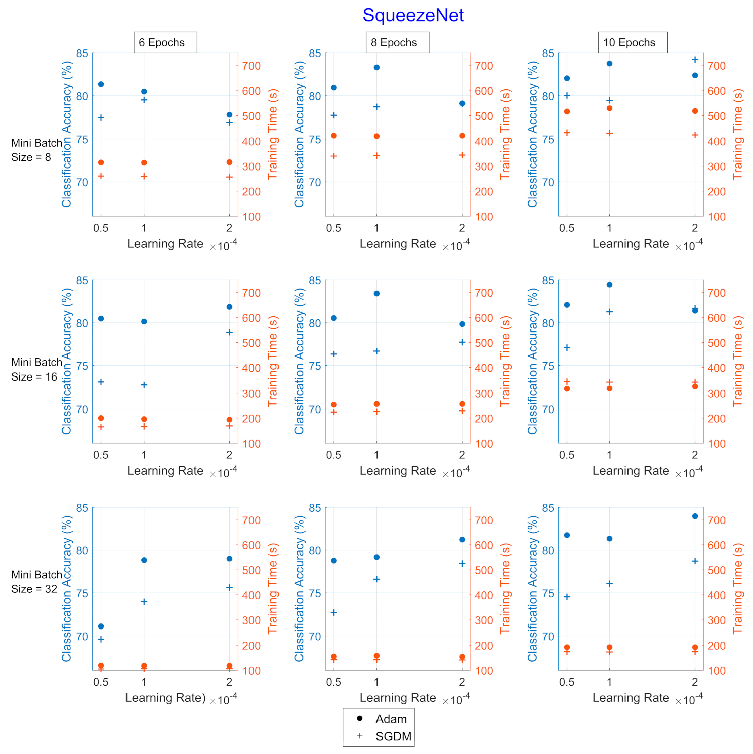
The three Image CNNs, GoogleNet, SqueezeNet, and ShuffleNet, were retrained using the 54 hyperparameter combinations, for the three datasets. The evaluation was based on the classification accuracy (CA) and the training time (TT). The three datasets followed a similar trend, and the results of the UrbanSound8k dataset are depicted in Figure 3, Figure 4 and Figure 5.

Adam optimizer performed better in terms of CA (blue color), while SGDM performed better in terms of TT (red color). Additionally, as the mini-batch size increased, the TT became shorter, and vice versa regarding the number of epochs, as expected. The learning rate, which affects how fast a network learns, has a direct impact on how well it learns, which makes this hyperparameter the most sensitive to set.

In all Image CNNs, Adam (blue dot) achieved better performance than SGDM (red dot). In

Table 7. Average values of CA and TT for each network for both optimizers for the UrbanSound8k dataset.

CNN	Adam		SGDM
	CA (%)	TT (s)	CA (%)	TT (s)
GoogleNet	85.28	691	78.60	505
SqueezeNet	80.98	277	77.22	268
ShuffleNet	86.70	1892	80.37	1381

, the networks are compared in terms of the average values of CA and TT for each optimizer for the UrbanSound8k dataset. SqueezeNet was the network with the shortest TT but also with the lowest CA. ShuffleNet presented the highest TT, approximately 2.7 times greater than the corresponding of GoogleNet.

The results for the remaining two datasets followed the same trend, as shown in

Table 8. Average values of CA and TT for each network for both optimizers for the ESC-10 dataset.

CNN	Adam		SGDM
	CA (%)	TT (s)	CA (%)	TT (s)
GoogleNet	84.10	33	78.75	24
SqueezeNet	79.49	15	70.28	13
ShuffleNet	82.22	112	73.29	87

and

Table 9. Average values of CA and TT for each network for both optimizers for the Air Compressor dataset.

CNN	Adam		SGDM
	CA (%)	TT (s)	CA (%)	TT (s)
GoogleNet	95.92	202	86.61	101
SqueezeNet	94.00	62	87.49	48
ShuffleNet	96.01	368	89.15	279

.

Sound CNNs:

Applying the nine combinations of hyperparameters upon the Sound CNNs, both VGGish and YAMNet exceeded 95% in CA for the UrbanSound8k dataset and reached 100% for the Air Compressor dataset. VGGish showed a marginally lower performance from the Image CNNs for the ESC-10 dataset, while YAMNet achieved a better performance from all Image CNNs. In terms of TT, both Sound networks showed a significant reduction, of 80% on average. The average values of CA and TT for all combinations for VGGish and YAMNet for the three datasets are shown in

Table 10. Average values of CA and TT for all combinations for VGGish and YAMNet for the three datasets.

CNN	CA (%)			TT (s)
	Urban Sound8k	ESC-10	Air Compressor	Urban Sound8k	ESC-10	Air Compressor
VGGish	95.68	82.36	99.97	253	18	45
YAMNet	96.24	88.06	100	797	55	151

.

4.2. Champion Hyperparameter Combinations

To select the most effective (‘champion’) combinations, we formed one conditional and one weight-based criterion. The former (conditional) required that a model outperformed in terms of both CA and TT than their average values by at least one standard deviation. The latter employed a weighted average of the (positive) difference of these parameters to the average values. The weight K allowed for normalization and prioritized the CA (by a factor of 2).

$$TT〈TTavg-TTstd \& CA〉CAavg+CAstd$$

(4)

$$\left(TTavg-TT\right)+K*\left(CA-CAavg\right), \mathrm{where} K=2*TTavg/CAavg$$

(5)

The most effective (‘champion’) combinations are presented in

Table 11. Most effective combinations of hyperparameters’ values for Image CNNs for each dataset.

Image CNNs	GoogleNet				SqueezeNet				ShuffleNet
Dataset	Optimizer	Mini Bach Size	Epochs	Learning Rate	Optimizer	Mini Bach Size	Epochs	Learning Rate	Optimizer	Mini Bach Size	Epochs	Learning Rate
Urban Sound8k	Adam	32	8	2	Adam	32	8	2	Adam	32	6	2
ESC-10	Adam	32	8	2	Adam	32	6	2	Adam	32	8	2
Air Compressor	Adam	32	10	2	Adam	32	6	2	Adam	32	8	2

for Image CNNs and in

Table 12. Most effective combinations of hyperparameters’ values for Sound CNNs for each dataset.

Sound CNNs	VGGish				YAMNet
Dataset	Optimizer	Mini Bach Size	Epochs	Learning Rate	Optimizer	Mini Bach Size	Epochs	Learning Rate
Urban Sound8k	Adam	256	4	2	Adam	256	4	2
ESC-10	Adam	256	5	2	Adam	256	5	2
Air Compressor	Adam	256	5	2	Adam	256	5	2

for Sound CNNs.

The investigation showed that Image CNNs were aligned in terms of the optimizer (Adam), the mini-batch size (32), and the learning rate ($2*{10}^{-4}$) for the three datasets. The number of epochs that affected the number of iterations in the training process differed among the datasets, which was directly related to the architecture of the network and the diversity of the data, e.g., recordings in various environments where other sounds were heard in the background or the tone was different.

For the Sound CNNs, VGGish and YAMNet agreed on the optimizer (Adam), the mini-batch size (256), and the learning rate ($2*{10}^{-4}$). Based on the ‘champion’ combinations, we performed classification in the test sound subset. To retrieve consistent results, the same set of pseudo-random test files were selected for all cases. For the case of image CNN, a set of scalogram images was selected, while for the case of Sound CNNs, the same subset of sound files was transformed into spectrograms. The training time corresponded to the training of $\left(60+20\right)\%$ of the files. The preprocessing time was the time needed to create the scalograms and the series of spectrograms for each file of the entire dataset for Image CNNs and Sound CNNs, respectively. For the creation of the scalograms, the preprocessing time was 11,172 s for the case of UrbanSound8k, 522 s for the ESC-10, and 432 s for the Air Compressor dataset. The results of classification accuracy (CA) and training time (TT) using Image CNNs for the three datasets are shown in

Table 13. Classification accuracy (CA) and training time (TT) for Image CNNs for each dataset.

Image CNNs	GoogleNet		SqueezeNet		ShuffleNet
Dataset	CA (%)	TT (s)	CA (%)	TT (s)	CA (%)	TT (s)
Urban Sound8k	87.06	348	83.97	192	87.18	780
ESC-10	86.25	17	83.75	7	87.50	53
Air Compressor	97.22	90	94.72	27	97.22	217

.

Another test was to feed the Image CNNs with the mel-spectrograms of the audio files saved as images suitable for the networks. This process took 6270 s (preprocess time) for UrbanSound8k and resulted in a 2.3% increase of CA and a 27.3% increase in TT on average. For the creation of the spectrograms, the preprocessing time was 783 s for UrbanSound8k, 9 s for the ESC-10, and 27 s for the Air Compressor dataset. The results of classification accuracy (CA) and training time (TT) using Sound CNNs for the three datasets are shown in

Table 14. Classification accuracy (CA) and training time (TT) for Sound CNNs for each dataset.

Sound CNNs	VGGish		YAMNet
Dataset	CA (%)	TT (s)	CA (%)	TT (s)
Urban Sound8k	96.70	210	96.16	603
ESC-10	91.25	16	91.25	36
Air Compressor	100	37	100	62

.

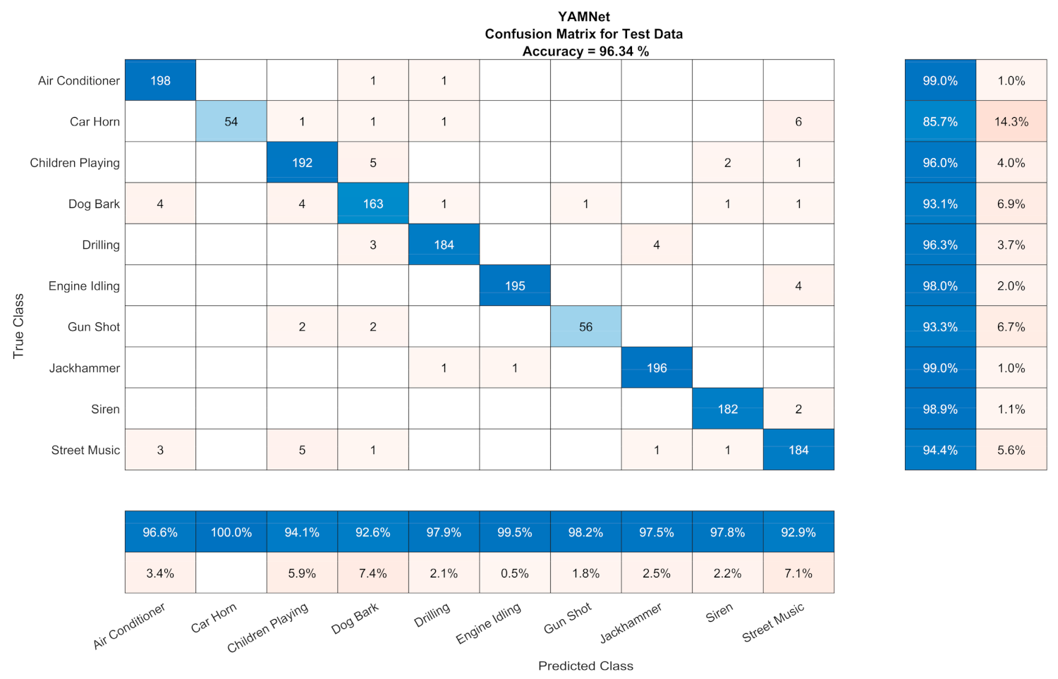
The CA results for the Sound CNNs for UrbanSound8k related to the subset of test files that had a duration larger than 0.96 s, which was the minimum segment in the case of segmentation (ESC-10 and Air Compressor had files that were 5 and 3 s long. respectively). In case we considered the rest of the test files for UrbanSound8k (i.e., those with a duration smaller than the minimum) as incorrect (non-existent) predictions, the CA were 92.05% and 91.99% for VGGish and YAMNet, respectively. Confusion matrices of the sound CNNs are depicted in Figure 6 and Figure 7 with the ‘champion’ hyperparameters.

Fusion:

The availability of multiple retrained networks allows for result combination (late fusion). We considered the following scenarios:

(1)

Majority-based selection, considering the three Image CNNs.

(2)

Majority-based selection, considering the five CNNs.

(3)

Enhancement of the best-performing Sound CNN (VGGish) with the results of the best-performing Image CNN (ShuffleNet), for the cases where the duration of the sound excerpts was beyond the necessary threshold.

(4)

Late fusion between the Sound CNNs after calculating the confidence level of each classification result. The confidence level was calculated as the ratio of the number of selected classifications per the total number of segments of the sound excerpt.

(5)

Late fusion of the Sound CNNs (using the confidence level) combined with the majority-based selection of the three Image CNNs for the sound excerpts with duration below the threshold.

The results per scenario for UrbanSound8k are presented in Figure 8.

5. Discussion

CNN application is extended from image-oriented research (including clustering classification and recognition) to sound research. The common denominator is the conversion of the sound signal into an image so that it is processed by the CNN. The CNN architecture evolution and design differences (ShuffleNet has 32% more layers than SqueezeNet) indicate that the design options are open and that there is no one-size-fits-all selection. While the number of layers initially followed an increasing tendency (leveraging the availability of increasing processing and memory resources), more effective designs have been brought forward. Two aspects can be considered in the usage of the CNNs:

(1) The relatively low ‘explainability’ of the sound transformation and representations within the CNN, in comparison with the classical ML methods where specific features are extracted, with their contributions being evaluated separately. This aspect is countervailed by the typically higher performance, in terms of classification accuracy, of the CNN architectures.

(2) The resource-consuming nature of the CNN training, when performed from scratch. The learning transfer paradigm is paving the way for even more effective, resource-friendly usage and ubiquitous deployment of CNNs.

Regarding the transformation of the sound signal into an image, different time-frequency transformations have been employed, namely scalograms (for SqueezeNet, GoogleNet, and ShuffleNet) and spectrograms (VGGish and YAMNet). In parallel, each sound excerpt can be transformed into a single image as in the case of Image CNNs or multiple images (corresponding to sound segments) as in the case of Sound CNNs. The latter allows for a more fine-grained classification evaluation while the homogeneity of the classification results (per segment) can be translated as the confidence level for the classification of the overall sound excerpt.

Transfer learning can have many flavors, in terms of reused and retrained parts while the retraining parameters (hyperparameters) influence the accuracy and the training time. Considering the training time and the classification accuracy (with appropriate weights), different criteria for hyperparameter selection can be formulated. Choosing the ‘champion’ hyperparameters’ combination can maximize the performance of a network according to the criterion considered.

We also compared the results of transfer learning with those achieved when training three of them from scratch. Specifically, we trained GoogleNet, SqueezeNet, and ShuffleNet from scratch using the three datasets (UrbanSound8K, ESC-10, and Air compressor) and the same number of epochs (employed for transfer learning). Each training used the ‘champion’ hyperparameter combinations.

The classification accuracy was less than that achieved with transfer learning, as depicted in Figure 9, on average by 27% for GoogleNet, 57% for SqueezeNet, and 25% for ShuffleNet. This is justified as effective training, typically requiring larger datasets and further repetitions for weight calculations. This observation amplifies the attractiveness of the transfer learning techniques.

6. Conclusions and Future Work

Sound classification is an ongoing problem and multiple techniques have been employed in this context, including classical methods based on explicit feature extraction and deep learning techniques (including CNNs). The latter (CNNs) offers better performance requiring increased (computational) resources, as verified with three datasets of different characteristics, in terms of classes and length.

Transfer learning techniques (applied upon CNNs) are an innovative and promising paradigm. The experimentation with three datasets and a considerable set of training configurations can allow for the selection of the most effective combination. The transfer learning paradigm was applied successfully, while it was observed that the re-training configurations can have a severe impact upon the classification accuracy and the computational resources required. Therefore, relevant investigation is recommended. Indications on the impact of the individual parameters considered were included.

The results of the tests performed, using the three datasets, indicate that Sound CNNs achieve better performance (as defined by the weighted combination of classification accuracy and training time) in comparison with Image CNNs. VGGish achieves the highest accuracy, with YAMNet following. Figure 10 depicts the classification accuracy per dataset and per CNN.

In terms of sound representation, equivalent image-based transforms (e.g., scalograms and spectrograms), in the case of already existing constraints and/or preferences, were verified to lead to similar results.

Fusion scenarios can also have positive results. Fusion can take place with a single classifier, through sound segmentation, independent classifications per segment, or fusion of the results, as pursued with the sound CNNs. Fusion can also take place if multiple classifiers are available, as a majority-based classification. For the UrbanSound8k dataset, the combination of the three Image CNNs exceeded the performance of the individual CNNs, while the fusion of all five networks was approximately the average of the combination of the three Image CNNs and the combination of the two Sound CNNs. The late fusion scenarios between VGGish and YAMNet with the majority-based selection of the three Image CNNs reached 96.28% classification accuracy.

The classification accuracy of the same CNNs upon different datasets allows for comparative observations in terms of the dataset quantity and quality, including sound segmentation and labeling precision as well as clearness of the types (or overlapping of multiple sounds). Regarding the three datasets we used, the Air Compressor had the best behavior as it gave the highest classification accuracy for all CNNs. This dataset had a smaller number of classes as well as limited number of audio files.

In terms of future work, we plan to continue the investigation of the transfer learning potential with additional datasets and CNNs. In parallel, we will further evaluate and compare transfer learning (upon CNNs already trained for initial datasets other than the dataset of interest) with training CNNs from scratch, employing different training configurations (learning rate, mini batch size, and epochs).