

Applying an Adaptive Neuro-Fuzzy Inference System to Path Loss Prediction in a Ruby Mango Plantation
1
Department of Electrical Engineering, Faculty of Engineering, Mahidol University, Nakhon Pathom 73170, Thailand
2
Department of Electrical Engineering and Energy Management, Faculty of Engineering, Kasem Bundit University, Bangkok 10250, Thailand
*
Author to whom correspondence should be addressed.
J. Sens. Actuator Netw. 2023, 12(5), 71; https://doi.org/10.3390/jsan12050071
Submission received: 25 July 2023
/
Revised: 23 September 2023
/
Accepted: 25 September 2023
/
Published: 7 October 2023
(This article belongs to the Topic Machine Learning in Communication Systems and Networks)
Abstract
:The application of wireless sensor networks (WSNs) in smart agriculture requires accurate path loss prediction to determine the coverage area and system capacity. However, fast fading from environment changes, such as leaf movement, unsymmetrical tree structures and near-ground effects, makes the path loss prediction inaccurate. Artificial intelligence (AI) technologies can be used to facilitate this task for training the real environments. In this study, we performed path loss measurements in a Ruby mango plantation at a frequency of 433 MHz. Then, an adaptive neuro-fuzzy inference system (ANFIS) was applied to path loss prediction. The ANFIS required two inputs for the path loss prediction: the distance and antenna height corresponding to the tree level (i.e., trunk and bottom, middle, and top canopies). We evaluated the performance of the ANFIS by comparing it with empirical path loss models widely used in the literature. The ANFIS demonstrated a superior prediction accuracy with high sensitivity compared to the empirical models, although the performance was affected by the tree level.
1. Introduction
A wireless sensor network (WSN) can be deployed in plantations to control the crop quality and quantity. However, the presence of trees and vegetation in the signal path can substantially degrade the performance of radio communication systems by causing signal attenuation, diffraction, scattering, and polarization [1]. Plantations comprise rows of densely foliated trees that can cause a significant path loss. Moreover, tree leaves tend to absorb water, which can cause further scattering of the signal. Low frequencies such as 240 MHz are less likely to be affected by weather conditions, such as rain and strong winds. Understanding path loss in the presence of vegetation is critical to the application of WSNs for smart agriculture.
Recently, empirical models, such as the log-distance and exponential decay models, have been developed for predicting the path loss around different types of vegetation in different frequency bands [2,3,4,5,6,7,8,9,10,11,12,13]. Raheemah et al. [2] proposed an empirical path loss model for a mango greenhouse at a frequency of 2.425 GHz with seven different antenna heights of 0.5, 1.0, 1.5, 2, 2.5, 3, and 3.5 m. The greenhouse contained 13 mango trees in three rows with a separation distance of 3.2 m between trees in the same row and 2.2 m between each row. The trees were 5 years old with a mean maximum height of 2 m, main trunk height of 1 m, and mean trunk diameter of 0.16 m. They demonstrated that their model had a better prediction accuracy than previous models in the literature. Anzum et al. [3] proposed a log-distance model with multiwall attenuation based on long-range (LoRa) measurement data at 433 MHz for oil palm trees planted in a symmetric pattern. Anderson et al. [4] characterized the path loss at a low antenna height (1.3 m) for ultrawideband propagation (830–4200 MHz) in four forest environments: light brush, light forest, medium forest, and dense forest. Azevedo et al. [5] proposed an empirical path loss model at frequencies of 870 and 2.414 MHz that considers the tree trunks of different trees. They multiplied the tree density and average trunk diameter to obtain a coefficient for the path loss exponent. Barrios-Ulloa et al. [6] reviewed log-distance and exponential decay models for the path loss at 200 MHz–95 GHz and compared their performances in terms of the root mean squared error (RMSE). Meng et al. [7,8] proposed a plane-earth model for near-ground wireless communication in the very high frequency (VHF) and ultrahigh-frequency (UHF) bands. They limited their interest to specific phenomena, such as the impact of near-ground or surface components on the signal propagation in different environments. Tang et al. [9] analyzed path loss models with the breakpoint distance on, near, and above the ground (heights of 5 cm, 50 cm, and 1 m, respectively) at a frequency of 470 MHz. Jong et al. [10] proposed a scattering model for a single oak tree at a frequency of 1.9 GHz. Pinto et al. [11] proposed a semi-deterministic model depending on the distance between transceivers of WSN nodes and the vegetation height for tomato greenhouses and demonstrated a superior prediction accuracy. Leonor et al. [12,13] proposed a raytracing scattering model for Ficus benjamina and Thuja pelicata trees at frequencies of 20 and 62.4 GHz.
Some researchers have used artificial intelligence (AI) technologies such as machine learning (ML) to improve the accuracy of empirical models in specific areas [14,15,16,17,18,19,20,21,22]. Chiroma et al. [14] reviewed the performances of AI models, such as support vector machines, neural networks (NNs), genetic algorithms, and the adaptive neuro-fuzzy interference system (ANFIS) in several types of communication environments: urban, suburban, and rural. Hakim et al. [15] developed ANFIS path loss models for forest, jungle, and open dirt road environments at frequencies of 433, 868, and 920 MHz and obtained a superior prediction accuracy compared to conventional empirical models. Faruk et al. [16] applied ML models including ANFIS to VHF and UHF bands in a typical urban environment and obtained a high prediction accuracy. Nunez et al. [17] showed that an artificial neural network (ANN) improved the prediction accuracy for indoor communication at 26.5–40 GHz [21]. Famoriji et al. [18] applied a backpropagation NN to path loss prediction in a tropical region and achieved a better prediction accuracy than a conventional log-distance model. Cruz et al. [19] applied an ANN and neuro-fuzzy system to the path loss prediction of a long-term evolution signal transmitted at a frequency of 1.8 GHz and compared the RMSE with those of commonly used empirical models in the literature. Wu et al. [20] applied a multilayer perceptron neural network (MLPNN) to predicting the path loss of three base stations at 2.5 GHz and achieved a better prediction accuracy than empirical log-distance models. Ostlin et al. [21] applied an ANN to predicting the path loss of a code-division multiple-access mobile network in a rural area and obtained good results. Egi et al. [22] proposed an ANN to predict the received signal level according to the detected tree canopy and location. Their model achieved an error of 4.26%, while the empirical model had an error of 6.29–16.9%.
Non-uniform vegetation is a common source of error for both empirical and intelligent path loss models. Some empirical models have been developed, providing a good prediction performance in uniform environments, such as an oil palm plantation and mango greenhouse. However, they still provided an error because of fast fading. The AI models are generally applied to specific non-uniform environments, such as urban, suburban, and rural areas, to improve the large errors at some measurement points. The models were trained with the measured data to provide a good prediction. However, in the case of a specific environment, such as the Ruby mango plantation, the AI model needs an expert system to create a rule base for training. Therefore, we applied an ANFIS in this study to predict the path loss of a signal in a Ruby mango plantation. Ruby mango trees are trimmed to limit their height and are planted in symmetric patterns for a uniform environment.
The ANFIS only requires two inputs: the distance and antenna height in relation to the tree level (i.e., trunk and canopy). The regular pattern of trees should allow the ANFIS to predict the path loss with high accuracy. To evaluate the performance of the proposed model, we compared it against existing empirical models. The contributions of this article are summarized as follows:
- An accurate semi-deterministic path loss prediction for a uniform Ruby mango plantation with an ANFIS engine, which consists of two inputs, namely, the distance between the transceivers of WSN nodes and vegetation height together, and an output of path loss prediction.
- The validation of the model using RMSE, MAE, and MAPE against benchmark models.
2. Related Path Loss Models
Four empirical models are widely used to predict the path loss considering vegetation and are presented here.
2.1. ITU-R Model
The International Telecommunications Union Recommendations (ITU-R) model [23] was developed from measurements mainly at the UHF band and was proposed for cases where either the transmit or receive antenna is near a small grove of trees through which the signal propagates. This model is commonly used for frequencies between 200 MHz and 95 GHz, and it is expressed as
where f is the frequency (MHz) and d is the tree depth.
2.2. COST 235 Model
The COST 235 model [24] is based on measurements at the millimeter-wave frequency band (9.6–57.6 GHz) through a small grove of trees performed over two seasons: when the trees were in-leaf and out-of-leaf. This model is also applicable to frequencies between 200 MHz and 95 GHz, and it is expressed by
2.3. FITU-R Model
The fitted ITU-R (FITU-R) model is based on datasets collected during the in-leaf and out-of-leaf states at 11.2 and 20 GHz [7]:
This model was developed because the lateral wave becomes dominant in both the VHF and UHF bands at relatively large forest depths, especially when both the transmit and receive antennas are inside the forest. Based on measurement data from an oil palm tree plantation, the FITU-R model becomes the following:
where f is the carrier frequency (MHz), is the height of the transmit antenna (m), is the height of the receive antenna (m), and d is the distance between the transmit and receive antennas (m). The model in (4) is for a theoretically free space, which can be used to obtain a reference model for estimating the path loss in different environments:
where f is the frequency (MHz) and d is the distance between the transmit and receive antennas (km). In a forest environment, Equation (5) can be modified to
For near-ground path loss, a plane-earth model is often used to consider both line-of-sight (LOS) and ground-reflected rays received by the receive antenna [7]:
where ht is the height of the transmit antenna (m), hr is the height of the receive antenna (m), and d is the distance between the transmit and receive antennas (m). If the excess loss is considered, then (6) becomes
Because of lateral wave propagation from diffraction over treetops and beside trees, especially in VHF and UHF bands, the effect induced by the perfect plane-earth model is reduced. Thus, the fitted ground reflection model becomes applicable:
where n is an empirical path loss exponent for LOS ground reflection. Then, the path loss model becomes
In this study, we used the path loss model in (6) because the excess loss (i.e., first term) includes the near-ground effect of different antenna heights. Table 1 summarizes the A, B, and C parameters.
2.4. Log-Distance Model
3. Proposed ANFIS Model
From the path loss model involved in Section 2, various empirical models have been developed. These empirical models are created using mathematical/statistical methods. In some cases, the environment is complex and finding a mathematical model is not easy. However, if a researcher has expertise in analyzing the nature of electromagnetic propagation, researchers can use that expertise to create fuzzy rules to predict the propagation of electromagnetic waves. This research proposes to use an ANFIS to generate fuzzy rules for path loss model prediction.
The ANFIS is a hybrid of an NN and fuzzy system, which is an inferential linguistic processing that incorporates fuzzy rules into a knowledge base [27]. The knowledge base contains fuzzy rules obtained from experts and can be adapted to produce appropriate results. However, the input–output pair must be learned to optimize the output. The NN is used to learn input–output relationships to adjust the fuzzy rules until a suitable output is found. Figure 1 shows the general architecture of an ANFIS, which has five main layers [28]. The rectangular boxes are adaptive nodes, while round boxes are fixed nodes.
Our ANFIS has two inputs and one output. Each input is divided into two fuzzy sets: A1, A2, and B1, B2. The output parameters are pj, qj, and rj, with n rules:
Rule 1: IF x1 is and x2 is THEN f1 = p1x1 + q1x2 + r1
Rule 2: IF x1 is and x2 is THEN f2 = p2x1 + q2x2 + r2
…
Rule n: IF x1 is and x2 is THEN fn = pnx1 + qnx2 + rn
- where, and are the fuzzy description of the input sets, and fj are the crisp description of the outputs.
Layer 1: This layer comprises antecedent parameters obtained via fuzzy determination from the Crisp input x to membership value or using the following membership function:
where is the membership of Ai derived from the input x. The membership function may be a triangular, inverted bell, or other shape.
Layer 2: This layer comprises the T-norm operator or fuzzy rule base, which associates fuzzy values from each dimension and sends the product as an output signal:
where is the firing strength from each rule and is the fuzzy value from the ith dimension of rule j.
Layer 3: This layer involves normalizing the firing strength or weighted layers so that all conditions from all rules can be combined into a single value:
Layer 4: The layer comprises consequent parameters obtained as follows:
Layer 5: This layer comprises the overall output, which includes all incoming signals and their defuzzification:
where = [ is the fuzzy value normalized from 1 − n rules and is the output of 1 − n rules.
From the proposed model, there are two major issues, as mentioned in Section 2 and Section 3: (1) the mathematical/statistical models, as in Section 2, and (2) the fact that the ANFIS is a black box method, and the fuzzy rules that are tuned from artificial neural networks (ANNs) are not easily understandable. Based on ANFIS concepts, many models have been proposed and applied to the subject of time series. The relationship between CO2 emissions from the energy sector and global temperature increases was investigated using ANFIS, ANN, and fuzzy time series models. This research aimed to avoid strict assumptions and study the complex relationships between variables [29]. A time series forecasting model using a hybrid method of an autoregressive adaptive network fuzzy inference system (AR-ANFIS) was studied. The AR-ANFIS was trained by using particle swarm optimization, and fuzzification was performed using the fuzzy C-Means method [30]. Multivariate time series prediction using a neuro-fuzzy model was proposed. Gaussian membership functions and a learning algorithm were used in the consequent layer [31]. The reviewed literature included training and optimization methods using complex functions and learning algorithms. This technique increases the complexity of the analysis. However, in this study path loss is determined based on a trajectory with a linear relationship between the variables. Therefore, this research uses linear relationships in layer 4 as consequent parameters. This is enough to create an accurate model. This section uses numerical data, which consist of distances, the height of the antenna, and the signal strength of electromagnetic waves. A collection of related datasets consists of a training dataset and a testing dataset. The training dataset is used to generate fuzzy rules and adjust the fuzzy set using a neural network. In general, the principle of fuzzy rules is to optimize the input set of rules in a given operating environment. Traditional methods use experts’ expertise to modify fuzzy rules. The ability to predict the results depend on the expert’s expertise. Furthermore, fuzzy rules can be created by simulating real situations to learn to create rules, which is inconvenient in the case of electromagnetic wave propagation. In this research, the fuzzy tuning setup has been developed using a neural network to achieve more accurate predictions. Adapting fuzzy rules will require training from the training data to optimize fuzzy sets and fuzzy rules, as detailed in the section above.
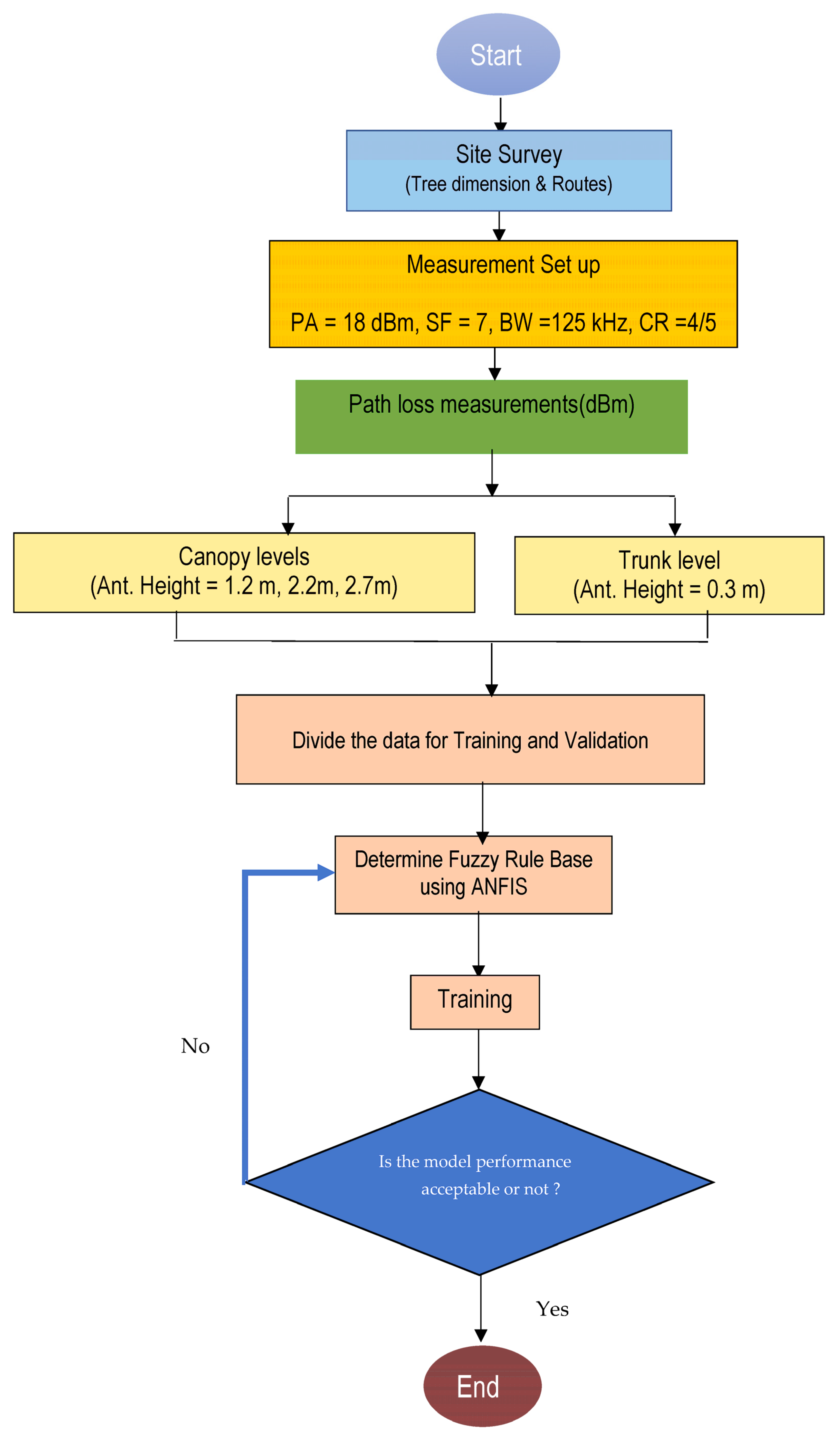
The antenna height and distance between the communication nodes influences the propagation path loss. Therefore, two inputs of the ANFIS are the antenna height in meters and logarithm of distance in meters. The output is the propagation path loss in dBm. A flowchart of the ANFIS path loss modeling is shown in Figure 2. The next section describes the site survey and measurement setup in detail.
4. Experimental
4.1. Study Site
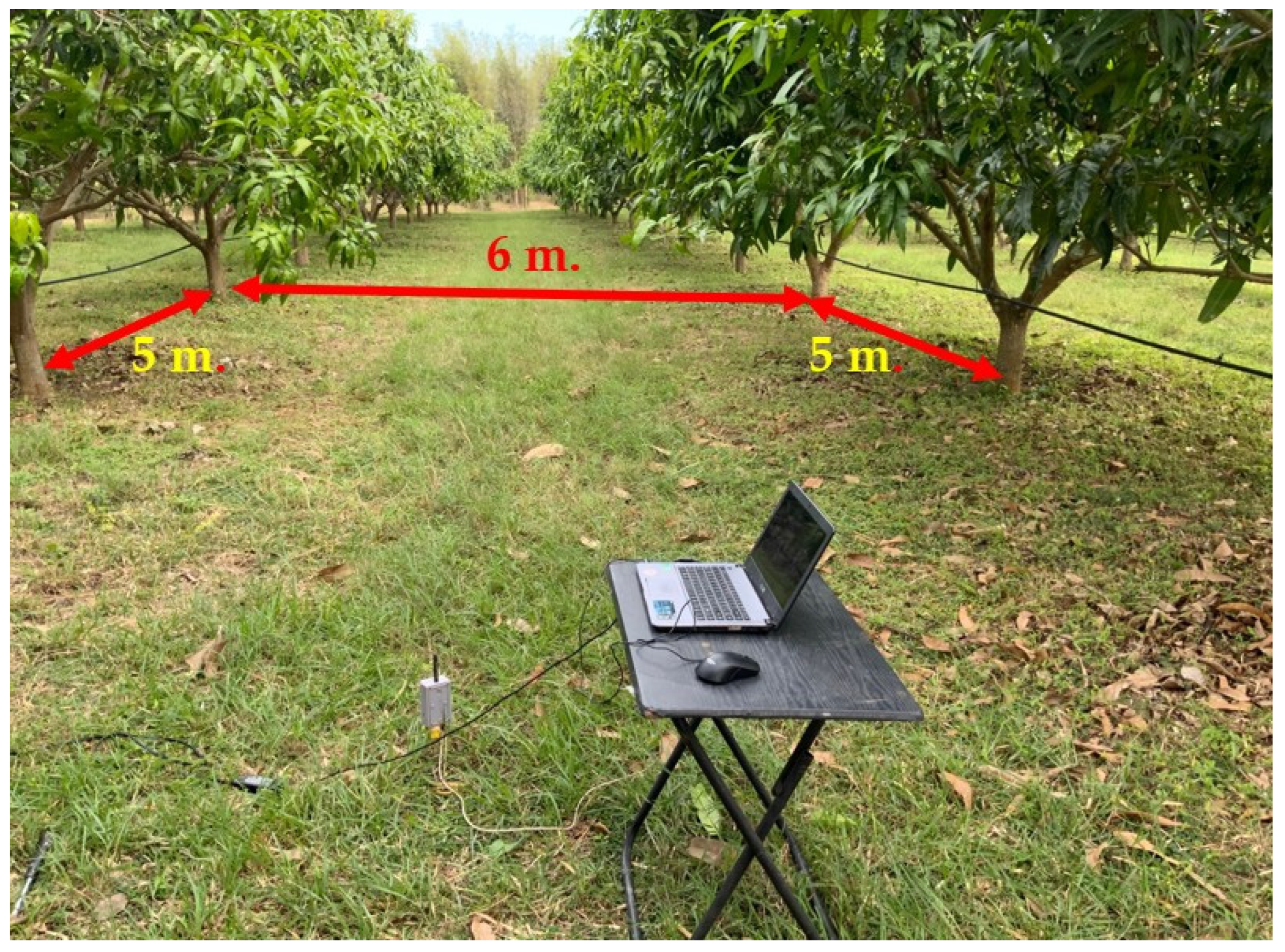
The study site was a Ruby mango plantation in Sakaeo Province, Thailand, with the GPS coordinates 13.4166954 N, 102.1368925 E. To ensure a good harvest, Ruby mango trees must be planted at a certain density. Thus, the mango tree plantation follows a specific pattern. The trees are planted in straight rows with 6 m between rows and 5 m between their trunks in the same row, as shown in Figure 3. The plantation has 320 trees per hectare. The tree dimensions are summarized in Table 2. The average total tree height was about 4.5 m, which comprised a trunk height of 0.55 m, a trunk diameter of 0.51 m, a canopy depth of 3.96 m, and an average canopy diameter of 5.69 m.
4.2. Measurement Setup
The measurement equipment comprised a fixed 433 MHz LoRa module (transceiver and omnidirectional antenna) as the receiving station and a portable LoRa module as the transmitter. These modules were connected to a microcontroller (Arduino board) that programmed the transmitter to send a data packet containing the word “hello” with the received signal strength indicator (RSSI) wirelessly to the receive antenna every 1.5 s. Three physical layer parameters were considered that influence the effective bit rate during modulation to cause noise and signal interference in a communication channel: the spreading factor (SF), bandwidth (BW), and coding rate (CR) [32].
Spreading factor: The SF is the ratio between the symbol rate and chip rate. A higher SF increases the sensitivity and transmission range with a lower packet error rate (PER) and RSSI, but it increases the airtime of the transmitted packet. Therefore, a lower SF should result in a higher PER and minimum RSSI.
Bandwidth: A higher BW increases the transmission range and data rate and thus decreases the airtime, but it also decreases the sensitivity by integrating additional noise. A lower BW increases the sensitivity but decreases the data rate. A typical LoRa network operates at a BW of 125, 250, or 500 kHz.
Coding rate: A LoRa network sets a CR to protect against bursts of interference. The CR is usually set to 4/5, 4/6, 4/7, or 4/8. A higher CR better protects the system against decoding errors by transmitting more redundant data bits but increases the airtime.
In this experiment, we only focused on the wave propagation characteristics of Ruby mango trees. Therefore, we used an SF of 7, BW of 125 kHz, and CR of 4/5 to increase the minimum RSSI, PER, sensitivity, and protection against decoding errors. The RSSI can be converted to the path loss by [33]
where K is an offset that depends on the characteristics of the transceiver chips used, the frequency, and the chosen technology and its features. However, K may be obtained via calibration. Table 3 summarizes the equipment parameters. To model the path loss, the RSSI data were captured via a notebook computer at the receiving station while the portable transmitting node was moved in 5 m intervals to a maximum distance of 40 m in both the forward and reverse directions. The heights of the transmit and receive antennas were set equal but varied at 0.3, 1.2, 2.2, and 2.7 m above the ground, as shown in Figure 4. Table 4 shows the path loss parameters of Equation (11), which was used for comparison with the ANFIS model.
The following metrics were used to evaluate the model performances based on their deviation from the measurement data: the absolute mean error (AME), mean absolute error (MAE), mean absolute percentage error (MAPE), and root mean square error (RMSE). These metrics were calculated as follows:
where is the measured path loss, is the predicted path loss, N is the total number of data, and the subscript i is the number of a given data.
5. Results and Discussion
5.1. ANFIS Model and Validation
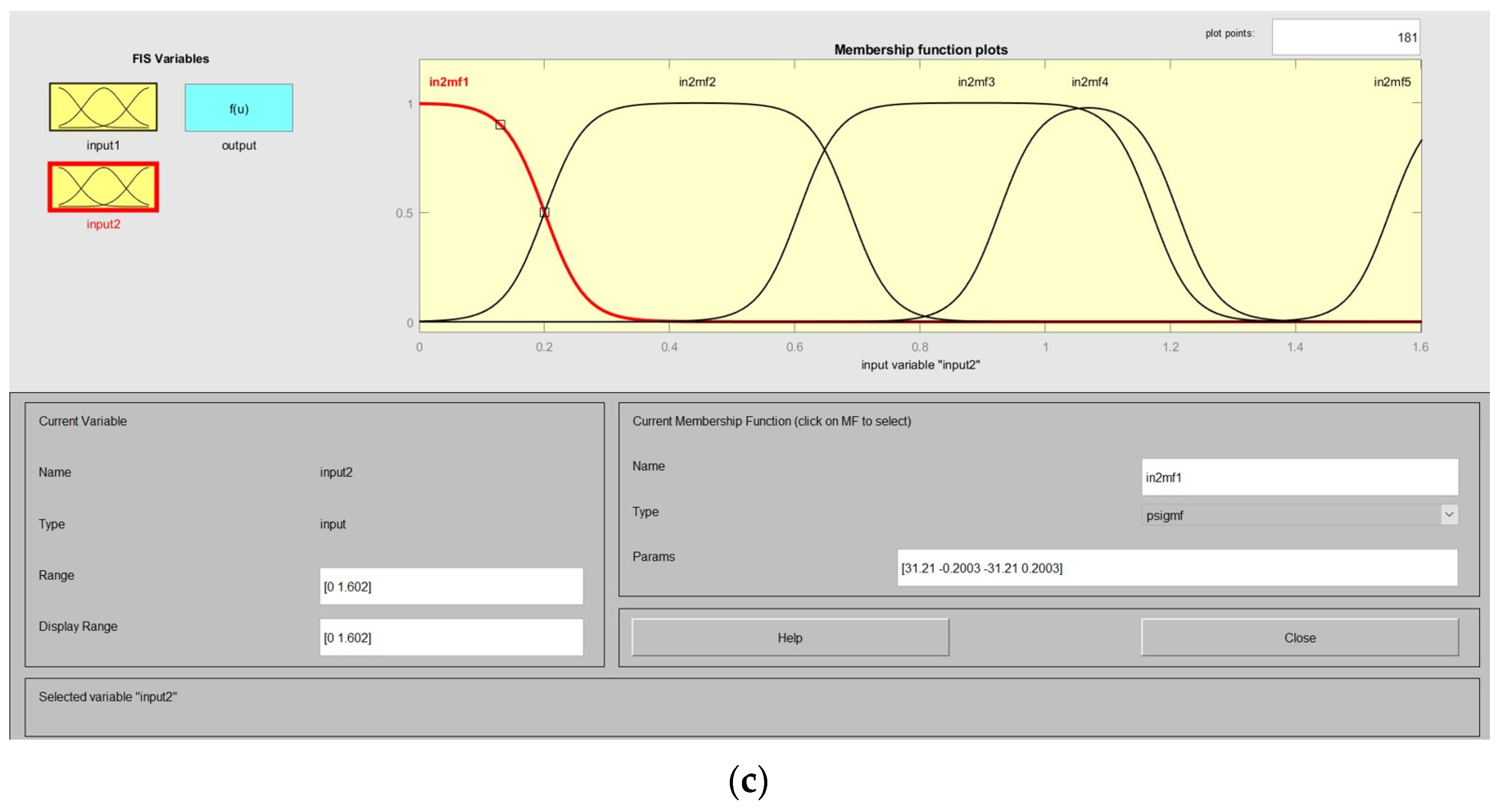
The measurement data described in Section 4 were used for the training and validation of the proposed ANFIS model. The training dataset comprised input–output data pairs, such as the antenna height (m), distance (m), and measured path loss (dB). A first-order Sugeno fuzzy model was used for the ANFIS structure, where the inputs were the antenna height and distance and the output was the path loss. The membership functions used the psigmf model with a mixed learning process (Hybrid), [5, 5] mfs, and 100 epochs for calculation. The results are shown in Figure 5 and Figure 6. The crisp input was divided into five fuzzy sets to obtain the minimum error. Each set contained {in1mf1, in1mf2, in1mf3, in1mf4, and in1mf5} for the antenna height input and {in2mf1, in2mf2, in2mf3, in2mf4, and in2mf5} for the log-distance input, and the output {out1mf1-out1mf25} was obtained according to the following 25 rules:
Rule 1: IF x1 is mf1 and x2 is mf1, THEN y is mf1
Rule 2: IF x1 is mf1 and x2 is mf2, THEN y is mf2
Rule 3: IF x1 is mf1 and x2 is mf3, THEN y is mf3
Rule 4: IF x1 is mf1 and x2 is mf4, THEN y is mf4
Rule 5: IF x1 is mf1 and x2 is mf5, THEN y is mf5
Rule 6: IF x1 is mf2 and x2 is mf1, THEN y is mf6
Rule 7: IF x1 is mf2 and x2 is mf2, THEN y is mf7
Rule 8: IF x1 is mf2 and x2 is mf3, THEN y is mf8
Rule 9: IF x1 is mf2 and x2 is mf4, THEN y is mf9
Rule 10: IF x1 is mf2 and x2 is mf5, THEN y is mf10
Rule 11: IF x1 is mf3 and x2 is mf1, THEN y is mf11
Rule 12: IF x1 is mf3 and x2 is mf2, THEN y is mf12
Rule 13: IF x1 is mf3 and x2 is mf3, THEN y is mf13
Rule 14: IF x1 is mf3 and x2 is mf4, THEN y is mf14
Rule 15: IF x1 is mf3 and x2 is mf5, THEN y is mf15
Rule 16: IF x1 is mf4 and x2 is mf1, THEN y is mf16
Rule 17: IF x1 is mf4 and x2 is mf2, THEN y is mf17
Rule 18: IF x1 is mf4 and x2 is mf3, THEN y is mf18
Rule 19: IF x1 is mf4 and x2 is mf4, THEN y is mf19
Rule 20: IF x1 is mf4 and x2 is mf5, THEN y is mf20
Rule 21: IF x1 is mf5 and x2 is mf1, THEN y is mf21
Rule 22: IF x1 is mf5 and x2 is mf2, THEN y is mf22
Rule 23: IF x1 is mf5 and x2 is mf3, THEN y is mf23
Rule 24: IF x1 is mf5 and x2 is mf4, THEN y is mf24
Rule 25: IF x1 is mf5 and x2 is mf5, THEN y is mf25
Figure 5a shows the ANFIS structure for training comprising five membership functions with the two adjusted inputs (Figure 5b,c) for 25 rules and 25 membership functions to obtain the output. Figure 6 shows the inference engine based on 25 rules with the first input as the antenna height of 1.2 m and the second input as the log-distance (d) of 0.698 (5 m), which provides a path loss output of 57.0 dB. Table 4 shows a good agreement of the ANFIS with validation.
5.2. Data Analysis of Proposed Model
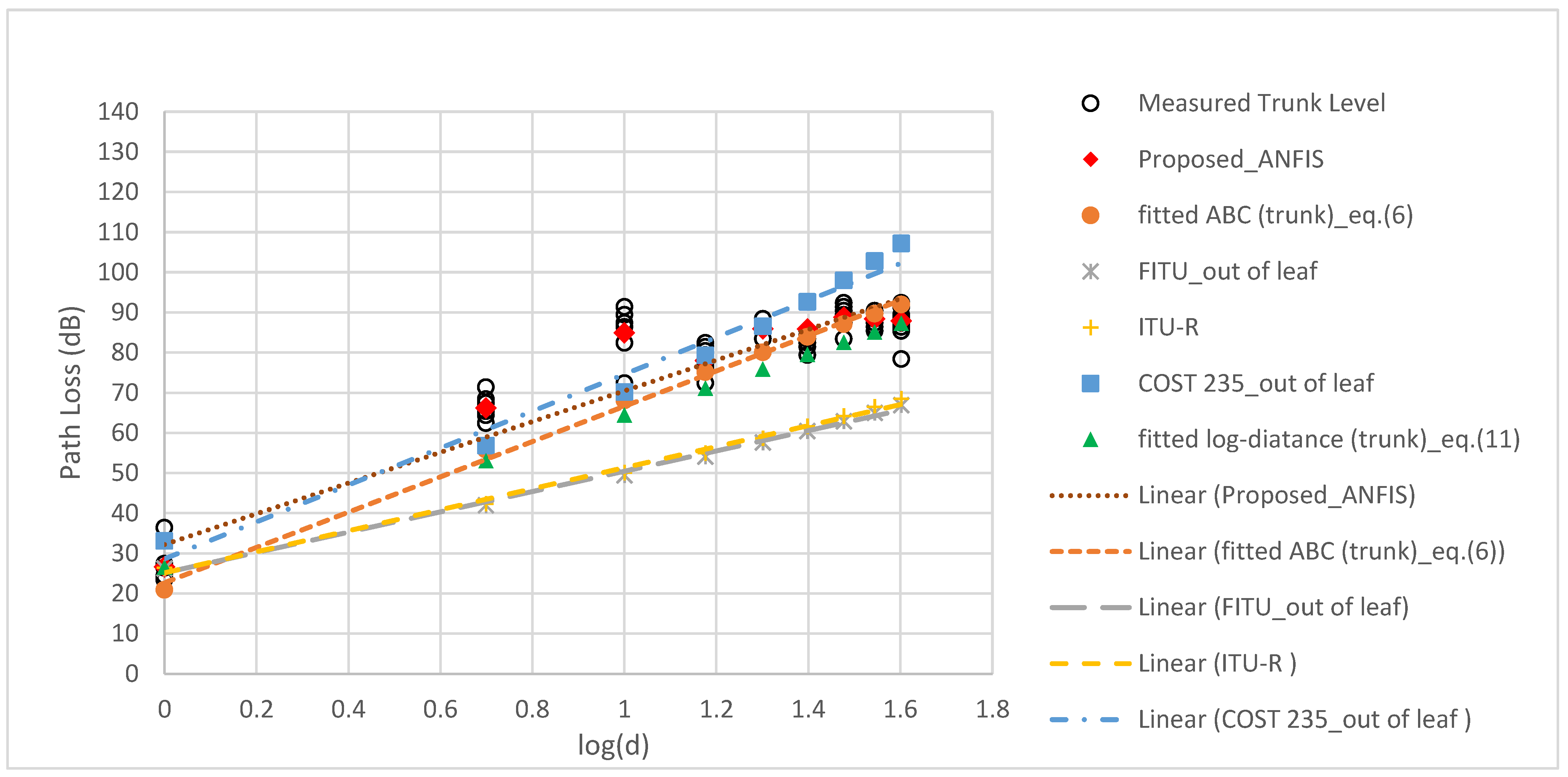
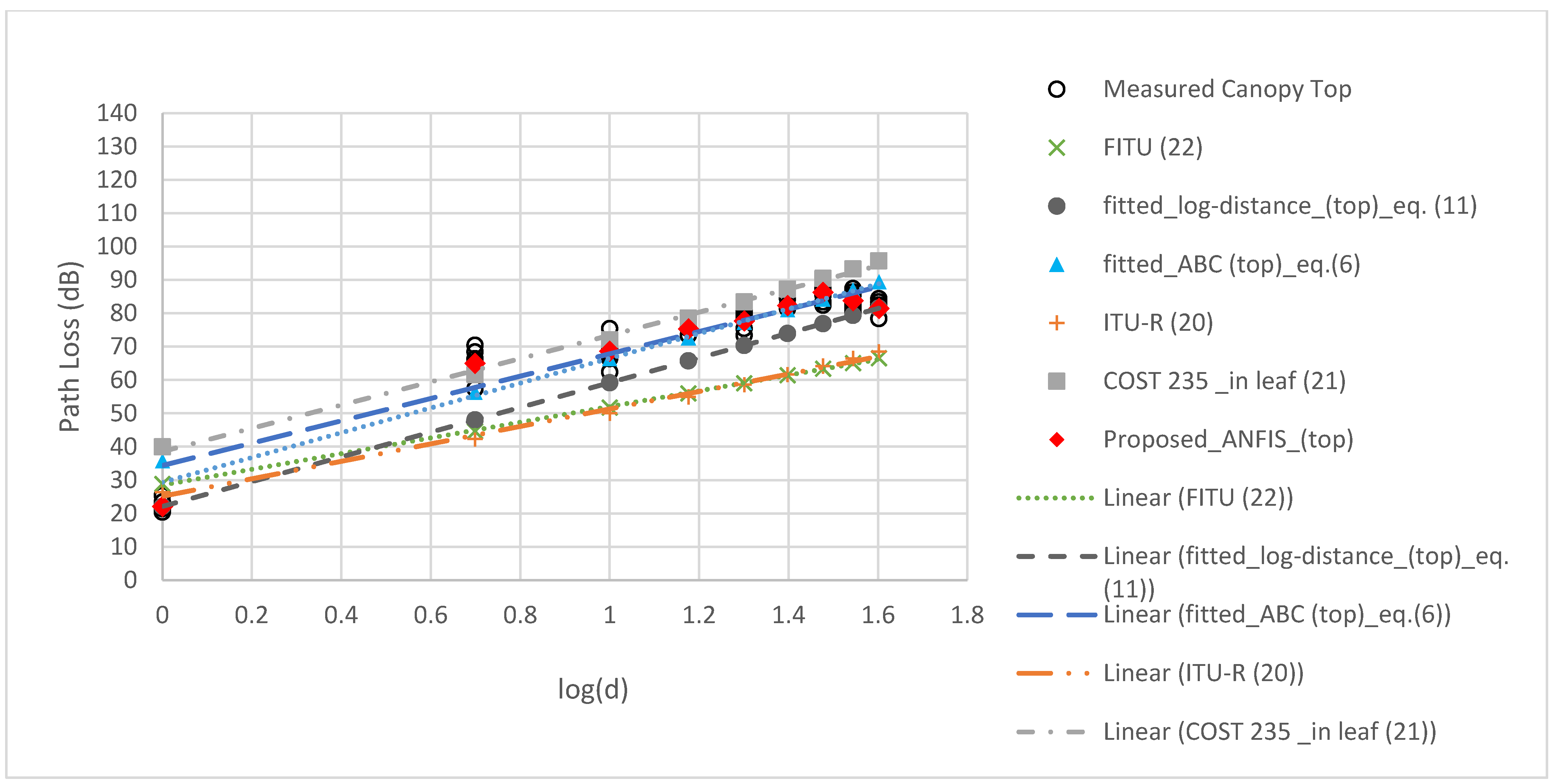
The performance of the proposed ANFIS was evaluated in terms of the metrics presented in Equations (18)–(21). Table 5, Table 6, Table 7 and Table 8 compare the ANFIS and measured data described in Section 4 according to the AME, MAE, MAPE, and RMSE, respectively. From the graphs in Figure 7, Figure 8, Figure 9 and Figure 10, the proposed ANFIS model can predict output values for the accurate estimation of measured path loss because mathematical models are obtained by averaging data to create a model. The real environment of the mango trees consists of different trunks and canopies. They are completely asymmetrical. Moreover, the wave attenuation value is not constant at each distance between the mango trees. It is difficult to find mathematic equations to explain these differences. However, the ANFIS model is a machine learning model that uses fuzzy rules to predict outcomes. The nature of the fuzzy rule depends on the linguistic variables used to describe the mango tree’s environment, which affects wave propagation. The fuzzy set is adjusted with a neural network to obtain the fuzzy sets with suitable values for prediction. Therefore, the ANFIS model makes predictions more accurate. Overall, the proposed ANFIS provided better prediction accuracy than the empirical models, especially at the bottom canopy, where it achieved AME, MAE, MAPE, and RMSE values of 0.01, 1.03, 1.64, and 1.34, respectively. However, it obtained a relatively large error at the trunk level with AME, MAE, MAPE, and RMSE values of 0.32, 2.43, 3.81, and 3.17, respectively. The MAE was smaller than the RMSE because of deviations in the measured path loss. The AME had the smallest values because the upper measurement data refuted the lower measurement data, while the MAPE had similar values to the RMSE.
5.3. Comparison with Empirical Path Loss Models
The ANFIS demonstrated good agreement with the measurement data compared with the empirical models in Section 2. The empirical model in Equation (6) provides the best prediction with an AME, MAE, MAPE, and RMSE values of 0.11, 0.77, 5.8, and 3.69, respectively (please see Table 5, Table 6, Table 7 and Table 8). In the case of the three conventional models, ITU-R (1), COST 235 (2), and FITU-R (3) provide large error prediction where either the transmit or receive antenna is near a small grove of trees. However, the COST 235 provides better prediction in the UHF band, as shown in Table 5, Table 6, Table 7 and Table 8, which the signal propagates at different antenna heights with the selected AME, MAE, MAPE, and RMSE values of 5.41, 6.86, 14.04, and 8.61, respectively. Additionally, the proposed ANFIS model provides a very high sensitivity compared with the empirical models, as indicated by the red dots in Figure 7, Figure 8, Figure 9 and Figure 10 for the trunk level and bottom, middle, and top canopy levels, respectively. These confirm the advantage of the proposed ANFIS model as well.
6. Conclusions
In this study, we applied an ANFIS to predict the path loss of a WSN in a Ruby mango plantation at 433 MHz. It is a combination of a neuro-fuzzy system and a learning algorithm. The ANFIS is able to learn from data and make predictions based on those data. The learning algorithm is able to adjust the weights of the connections between the neurons in the network and the parameters of fuzzy sets. This allows the ANFIS to learn and adapt to new data. We performed path loss measurements with two transceiver nodes between the trees at difference antenna heights. The ANFIS requires two inputs to predict the path loss: the antenna height corresponding to the tree level and the distance between the transmitter and receiver nodes. Each input was classified into five adjected fuzzy sets. The influence engine with 25 rule bases predicted the path loss with minimum error. We compared the performance of the proposed ANFIS with empirical models. The results showed that the proposed ANFIS demonstrated a superior prediction accuracy and high sensitivity with the best AME, MAE, MAPE, and RSME values of 0.01, 1.03, 1.64, and 1.34, respectively, at the antenna height of 1.2 m above ground (canopy bottom), although the performance fluctuated with the tree level. In future work, the capacity of the ANFIS will be improved to predict the path loss of inflorescence and fruit on tree, especially at a frequency of 2.4 GHz with a wave length of approximately 0.125 cm, which is smaller than the dimension of the inflorescence and fruit. This will significantly improve the signal attenuation, enabling the detection of inflorescence and fruit using the ANFIS for monitoring as well. The advantage of the ANFIS model is that is combines both numerical and linguistic knowledge. The ANN ability of the ANFIS is used to classify data and identify patterns. Compared to the ANN, the ANFIS model is more transparent to the user and causes less recognition errors.
Future research could extend the intelligence model by using a larger dataset to examine if better predictions can be obtained. The number of inputs in terms of attendance determinants, type of tree, difference frequency of wireless nodes, and amount of data can be expanded to develop more accurate and intelligent models and several applications.
Author Contributions
Conceptualization, S.P. and P.P.; methodology, S.P.; software, P.P.; validation, P.P.; formal analysis, S.P. and P.P.; investigation, S.P. and P.P.; resources, S.P. and P.P.; data curation, S.P.; writing—original draft preparation, S.P.; writing—review and editing, S.P.; visualization, S.P. and P.P.; supervision, P.P.; project administration, S.P.; funding acquisition, S.P. All authors have read and agreed to the published version of the manuscript.
Funding
Mahidol University for APC.
Data Availability Statement
Not applicable.
Acknowledgments
The authors thank Orapin Pitaksakorn for allowing them to conduct experiments in the Ruby mango plantation.
Conflicts of Interest
The authors declare no conflict of interest.
References
- Attenuation in Vegetation, Radiocommunication Assembly, document ITU-R P.833-8, ITU-R, 2013.
- Raheemah, A.; Sabri, N.; Salim, M.S.; Ehkan, P.; Ahmad, R.B. New empirical path loss model for wireless sensor networks in mango greenhouses. Comput. Electron. Agric. 2016, 127, 553–560. [Google Scholar] [CrossRef]
- Anzum, R.; Habaebi, M.H.; Islam, R.; Hakim, G.P.N.; Khandaker, M.U.; Osman, H.; Alamri, S.; Elrahim, E.A. A multiwall path-loss prediction model using 433 MHz LoRa-WAN frequency to characterize foliage’s in-fluence in a Malaysian palm oil plantation environment. Sensors 2022, 22, 5397. [Google Scholar] [CrossRef] [PubMed]
- Anderson, C.R.; Volos, H.I.; Buehrer, R.M. Characterization of low-antenna ultrawideband propagation in a forest environment. IEEE Trans. Veh. Technol. 2013, 62, 2878–2895. [Google Scholar] [CrossRef]
- Azevedo, J.; Santos, F.E.S. An empirical propagation model for forest environments at tree trnk level. IEEE Trans. Antennas Propag. 2011, 59, 2357–2367. [Google Scholar] [CrossRef]
- Barrios-Ulloa, A.; Ariza-Colpas, P.P.; Sánchez-Moreno, H.; Quintero-Linero, A.P.; De la Hoz-Franco, E. Modeling radio wave propagation for wireless sensor networks in vegetated environments: A systematic literature review. Sensors 2022, 22, 5285. [Google Scholar] [CrossRef]
- Meng, Y.S.; Lee, Y.H.; Ng, B.C. Empirical near ground path loss modeling in a forest at VHF and UHF bands. IEEE Trans. Antennas Propag. 2009, 57, 1461–1468. [Google Scholar] [CrossRef]
- Meng, Y.S.; Lee, Y.H. Investigations of foliage effect on modern wireless communication systems: A review. Prog. Electromagn. Res. 2010, 105, 313–332. [Google Scholar] [CrossRef]
- Tang, W.; Ma, X.; Wei, J.; Wang, Z. Measurement and analysis of near-ground propagation models under different terrains for wireless sensor networks. Sensors 2019, 19, 1901. [Google Scholar] [CrossRef]
- de Jong, Y.L.C.; Herben, M.H.A.J. A tree-scattering model for improved propagation prediction in urban microcells. IEEE Trans. Veh. Technol. 2004, 53, 503–513. [Google Scholar] [CrossRef]
- Pinto, D.C.; Damas, M.; Holgado-Terriza, J.A.; Arrabal-Campos, F.M.; Gómez-Mula, F.; Martínez-Lao, J.A.M.; Cama-Pinto, A. Empirical Model of Radio Wave Propagation in the Presence of Vegetation inside Greenhouses Using Regularized Regressions. Sensors 2020, 20, 6621. [Google Scholar] [CrossRef]
- Leonor, N.; Caldeirinha, R.; Fernandes, T.; Ferreira, D.; Sánchez, M.G. A 2D ray-tracing based model for micro-and millimeter-wave propagation through vegetation. IEEE Trans. Antennas Propag. 2014, 62, 6443–6453. [Google Scholar] [CrossRef]
- Leonor, N.; Sánchez, R.M.G.; Fernandes, T.; Ferreira, D. A 2D ray-tracing based model for wave propagation through forests at micro and millimeter wave frequencis. IEEE Access 2018, 6, 32097–32108. [Google Scholar] [CrossRef]
- Chiroma, H.; Nickolas, P.; Faruk, N.; Alozief, E.; Olayinkaf, I.F.Y.; Adewole, K.S.; Abdulkarimh, A.; Oloyedef, A.A.; Sowandef, O.A.; Garbai, S.; et al. Large scale survey for radio propagation in developing machine learning model for path losses in communication systems. Sci. Afr. J. 2023, 19, e01550. [Google Scholar] [CrossRef]
- Hakim, G.P.N.; Habaebi, M.H.; Toha, S.F.; Islam, M.R.; Yusoff, S.H.B.; Adesta, E.Y.T.; Anzum, R. Near Ground Pathloss Propagation Model Using Adaptive Neuro Fuzzy Inference System for Wireless Sensor Network Communication in Forest, Jungle and Open Dirt Road Environments. Sensors 2022, 22, 3267. [Google Scholar] [CrossRef]
- Faruk, N.; Popoola, S.I.; Surajudeen-Bakinde, N.T.; Oloyede, A.A.; Abulkarim, A.; Olawoyin, L.A.; Ali, M.; Calafate, C.T.; Atayero, A.A. Path Loss predictions in the VHF and UHF bands within urban environments: Experimental investigation of empirical, heuristics and geospatial models. IEEE Access 2019, 7, 77293–77307. [Google Scholar] [CrossRef]
- Nunez, Y.; Lovisolo, L.; Mello, L.S.; Orihuela, C. Path-Loss Prediction of Millimeter-wave using Machine Learning Techniques. In Proceedings of the 2022 IEEE Latin-American Conference on Communications (LATINCOM), Rio de Janeiro, Brazil, 30 November–2 December 2022; pp. 1–4. [Google Scholar]
- Famoriji, O.J.; Shongwe, T. Path loss prediction in Tropical regions using machine learning techniques: A case study. Electronics 2022, 11, 2711. [Google Scholar] [CrossRef]
- Cruz, H.A.O.; Nascimento, R.N.A.; Araujo, J.P.L.; Pelaes, E.G.; Cavalcante, G.P.S. Methodologies for path loss prediction in LTE-1.8 GHz networks using neuro-fuzzy and ANN. In Proceedings of the 2017 SBMO/IEEE MTT-S International Microwave and Optoelectronics Conference (IMOC), Aguas de Lindoia, Brazil, 27–30 August 2017. [Google Scholar]
- Wu, L.; He, D.; Ai, B.; Wang, J.; Qi, H.; Guan, K.; Zhong, Z. Artificial Neural Network Based Path Loss Prediction for Wireless Communication Network. IEEE Access 2020, 8, 199523–199538. [Google Scholar] [CrossRef]
- Ostlin, E.; Zepernick, H.J.; Suzuki, H. Macro cell Path-Loss Prediction Using Artificial Neural Networks. IEEE Trans. Veh. Technol. 2010, 59, 2735–2747. [Google Scholar] [CrossRef]
- Egi, Y.; Otero, C.E. Machine-Learning and 3D Point-Cloud Based Signal Power Path Loss Model for the Deployment of Wireless Communication Systems. IEEE Access 2019, 7, 42507–42517. [Google Scholar] [CrossRef]
- CCIR. Influences of Terrain Irregularities and Vegetation on Troposphere Propagation; CCIR: Geneva, Switzerland, 1986; pp. 235–236, CCIR Rep. [Google Scholar]
- European Commission. COST 235: Radio Propagation Effects on Next-Generation Fixed-Service Terrestrial Telecommunication Systems; European Union: Luxembourg, 1996; Final Rep. [Google Scholar]
- Parsons, J.D. The Mobile Radio Propagation Channel, 2nd ed.; Wiley: New York, NY, USA, 2000. [Google Scholar]
- Rappaport, T.S. Wireless Communication; Prentic Hall Publishers: Upper Saddle River, NJ, USA, 1996. [Google Scholar]
- Zadeh, L.A. The Concept of a Linguistic Variable and its Application to Approximate Reasoning. Inf. Sci. 1975, 8, 199–249. [Google Scholar] [CrossRef]
- Jang, J.S.R. ANFIS: Adaptive-Network-Based Fuzzy Inference System. IEEE Trans. Syst. Man Cybern. 1993, 23, 665–685. [Google Scholar] [CrossRef]
- Khan, M.Z.; Khan, M.F. Application of ANFIS, ANN, and fuzzy time series models to CO2 emission from the energy sector and global temperature increase. Int. J. Clim. Chang. Strateg. Manag. 2019, 11, 622–642. [Google Scholar] [CrossRef]
- Sarıca, B.; Eğrioğlu, E.; Aşıkgil, B. A new hybrid method for time series forecasting: AR–ANFIS. Neural Comput. Appl. 2018, 29, 749–760. [Google Scholar] [CrossRef]
- Vlasenko, A.; Vlasenko, N.; Vynokurova, O.; Peleshko, D. A Novel Neuro-Fuzzy Model for Multivariate Time-Series Prediction. Data 2018, 3, 62. [Google Scholar] [CrossRef]
- Citoni, B.; Fioranelli, F.; Imran, M.A.; Abbasi, Q.H. Internet of Things and LoRaWAN-Enabled Future Smart Farming. IEEE Internet Things Mag. 2019, 2, 14–19. [Google Scholar] [CrossRef]
- Onykiienko, Y.; Popovych, P.; Yaroshenko, R.; Mitsukova, A.; Beldyagina, A.; Makarenko, Y. Using RSSI data for LoRa network path loss modeling. In Proceedings of the 2022 IEEE 41st International Conference on Electronics and Nanotechnology (ELNANO), Kyiv, Ukraine, 10–14 October 2022; pp. 576–580. [Google Scholar]
Figure 1.
General architecture of the ANFIS.

Figure 2.
Flowchart of the ANFIS path loss model.

Figure 3.
Plan of Ruby mango plantation.

Figure 4.
Propagation measurement.

Figure 5.
ANFIS with two inputs: (a) structure, (b) antenna height as input 1, and (c) log-distance as input 2.
Figure 5.
ANFIS with two inputs: (a) structure, (b) antenna height as input 1, and (c) log-distance as input 2.


Figure 6.
Inference engine.

Figure 7.
Predicted and observed path losses at an antenna height of 0.3 m (trunk).

Figure 8.
Predicted and observed path losses at an antenna height of 1.2 m (bottom canopy).

Figure 9.
Predicted and observed path losses at an antenna height of 2.2 m (middle canopy).

Figure 10.
Predicted and observed path losses at an antenna height of 2.7 m (top canopy).


Table 1.
Path loss exponent parameters at 433 MHz (SF 7, BW 125 kHz).
| Antenna Height (m) | (dB) | PLE (NLOS) | A | B | C |
|---|---|---|---|---|---|
| 0.3 | 26.57 | 3.79 | 0.98 | 0.39 | 0.34 |
| 1.2 | 23.2 | 3.84 | 0.8 | 0.39 | 0.35 |
| 2.2 | 17.54 | 4.33 | 0.98 | 0.39 | 0.33 |
| 2.7 | 22.1 | 3.71 | 1.0 | 0.39 | 0.3 |
Table 2.
Measured dimensions of Ruby mango trees.
| No. | Total Height | Trunk Height | Trunk Diameter | Canopy Depth | Canopy Diameter |
|---|---|---|---|---|---|
| Tree 1 | 3.82 | 0.56 | 0.4 | 3.4 | 5.5 |
| Tree 2 | 4.66 | 0.66 | 0.56 | 4.0 | 6.0 |
| Tree 3 | 4.79 | 0.49 | 0.45 | 4.3 | 5.6 |
| Tree 4 | 5.15 | 0.65 | 0.64 | 4.5 | 6.5 |
| Tree 5 | 4.77 | 0.47 | 0.63 | 4.3 | 6.2 |
| Tree 6 | 3.96 | 0.46 | 0.46 | 3.5 | 4.7 |
| Tree 7 | 4.85 | 0.65 | 0.54 | 4.2 | 6.0 |
| Tree 8 | 3.97 | 0.47 | 0.43 | 3.5 | 5.0 |
| Average | 4.50 | 0.55 | 0.51 | 3.96. | 5.69 |
All numerical values are in meters.
Table 3.
Parameter setup.
| No. | Parameters | Value | Unit |
|---|---|---|---|
| 1 | Power amplifier (PA) | 18 | dBm |
| 2 | Antenna gain | 2.2 | dBi |
| 3 | Frequency | 433 | MHz |
| 4 | Bandwidth (BW) | 125 | kHz |
| 5 | Spreading factor | 7 | - |
| 6 | Code rate (CR) | 4/5 | - |
| 7 | Offset factor (K) | 28 | dBm |
Table 4.
RMSE of ANFIS model and validation.
| Antenna Height (m) | ANFIS Validation | |
|---|---|---|
| 0.3 (Trunk) | 3.17 | 3.31 |
| 1.2 (Canopy_bottom) | 1.34 | 1.58 |
| 2.2 (Canopy_middle) | 1.65 | 1.57 |
| 2.7 (Canopy_top) | 2.61 | 2.60 |
Table 5.
Model comparison using AME.
| Antenna Height (m) | AME | |||||
|---|---|---|---|---|---|---|
| Exponential Decay Equation (6) | Log-Distance Equation (11) | ITU-R | COST235 | FITU-R | ANFIS | |
| 0.3 (Trunk) | 0.11 | 5.73 | 19.33 | 5.41 | 20.26 | 0.32 |
| 1.2 (Canopy_bottom) | 0.28 | 3.14 | 15.91 | 7.91 | 15.69 | 0.01 |
| 2.2 (Canopy_middle) | 1.71 | 5.36 | 17.64 | 5.76 | 17.24 | 0.06 |
| 2.7 (Canopy_top) | 0.77 | 7.3 | 16.82 | 6.54 | 16.47 | 0.02 |
Table 6.
Model comparison using MAE.
| Antenna Height (m) | MAE | |||||
|---|---|---|---|---|---|---|
| Exponential Decay Equation (6) | Log-Distance Equation (11) | ITU-R | COST235 | FITU-R | ANFIS | |
| 0.3 (Trunk) | 6.17 | 6.32 | 19.63 | 10.19 | 20.55 | 2.43 |
| 1.2 (Canopy_bottom) | 2.66 | 3.36 | 16.39 | 7.91 | 16.49 | 1.03 |
| 2.2 (Canopy_middle) | 4.71 | 5.52 | 19.08 | 6.86 | 19.09 | 1.27 |
| 2.7 (Canopy_top) | 0.77 | 7.61 | 17.69 | 7.45 | 17.84 | 2.08 |
Table 7.
Model Comparison Using MAPE.
| Antenna Height (m) | MAPE | |||||
|---|---|---|---|---|---|---|
| Exponential Decay Equation (6) | Log-Distance Equation (11) | ITU-R | COST235 | FITU-R | ANFIS | |
| 0.3 (Trunk) | 11.91 | 8.89 | 25.09 | 15.49 | 26.20 | 3.81 |
| 1.2 (Canopy_bottom) | 5.8 | 4.9 | 22.3 | 14.04 | 22.73 | 1.64 |
| 2.2 (Canopy_middle) | 12.48 | 7.51 | 27.57 | 17.11 | 28.22 | 1.76 |
| 2.7 (Canopy_top) | 11.08 | 10.51 | 24.42 | 15.5 | 25.28 | 3.16 |
Table 8.
Model comparison using RMSE.
| Antenna Height (m) | RMSE | |||||
|---|---|---|---|---|---|---|
| Exponential Decay Equation (6) | Log-Distance Equation (11) | ITU-R | COST235 | FITU-R | ANFIS | |
| 0.3 (Trunk) | 7.74 | 8.59 | 21.65 | 11.77 | 22.59 | 3.17 |
| 1.2 (Canopy_bottom) | 3.69 | 4.08 | 16.96 | 8.61 | 17.1 | 1.34 |
| 2.2 (Canopy_middle) | 6.7 | 7.05 | 19.84 | 8.63 | 19.87 | 1.65 |
| 2.7 (Canopy_top) | 6.52 | 9.1 | 18.62 | 9.09 | 18.53 | 2.61 |
Disclaimer/Publisher’s Note: The statements, opinions and data contained in all publications are solely those of the individual author(s) and contributor(s) and not of MDPI and/or the editor(s). MDPI and/or the editor(s) disclaim responsibility for any injury to people or property resulting from any ideas, methods, instructions or products referred to in the content. |
© 2023 by the authors. Licensee MDPI, Basel, Switzerland. This article is an open access article distributed under the terms and conditions of the Creative Commons Attribution (CC BY) license (https://creativecommons.org/licenses/by/4.0/).
Share and Cite
MDPI and ACS Style
Phaiboon, S.; Phokharatkul, P. Applying an Adaptive Neuro-Fuzzy Inference System to Path Loss Prediction in a Ruby Mango Plantation. J. Sens. Actuator Netw. 2023, 12, 71. https://doi.org/10.3390/jsan12050071
AMA Style
Phaiboon S, Phokharatkul P. Applying an Adaptive Neuro-Fuzzy Inference System to Path Loss Prediction in a Ruby Mango Plantation. Journal of Sensor and Actuator Networks. 2023; 12(5):71. https://doi.org/10.3390/jsan12050071
Chicago/Turabian StylePhaiboon, Supachai, and Pisit Phokharatkul. 2023. "Applying an Adaptive Neuro-Fuzzy Inference System to Path Loss Prediction in a Ruby Mango Plantation" Journal of Sensor and Actuator Networks 12, no. 5: 71. https://doi.org/10.3390/jsan12050071
Note that from the first issue of 2016, this journal uses article numbers instead of page numbers. See further details here.