


On Maximizing the Probability of Achieving Deadlines in Communication Networks

1
Multimedia Communications Lab (KOM), Department of Electrical Engineering and Information Technology, Technical University of Darmstadt, 64283 Darmstadt, Germany
2
Department of Electrical Engineering, Pontificia Universidad Católica de Chile, Santiago 7820436, Chile
*
Authors to whom correspondence should be addressed.
J. Sens. Actuator Netw. 2024, 13(1), 9; https://doi.org/10.3390/jsan13010009
Submission received: 1 December 2023
/
Revised: 6 January 2024
/
Accepted: 15 January 2024
/
Published: 18 January 2024
(This article belongs to the Topic Electronic Communications, IOT and Big Data)
Abstract
:We consider the problem of meeting deadline constraints in wireless communication networks. Fulfilling deadlines depends heavily on the routing algorithm used. We study this dependence generically for a broad class of routing algorithms. For analyzing the impact of routing decisions on deadline fulfillment, we adopt a stochastic model from operations research to capture the source-to-destination delay distribution and the corresponding probability of successfully delivering data before a given deadline. Based on this model, we propose a decentralized algorithm that operates locally at each node and exchanges information solely with direct neighbors in order to determine the probabilities of achieving deadlines. A modified version of the algorithm also improves routing tables iteratively to progressively increase the deadline achievement probabilities. This modified algorithm is shown to deliver routing tables that maximize the deadline achievement probabilities for all nodes in a given network. We tested the approach by simulation and compared it with routing strategies based on established metrics, specifically the average delay, minimum hop count, and expected transmission count. Our evaluations encompass different channel quality and small-scale fading conditions, as well as various traffic load scenarios. Notably, our solution consistently outperforms the other approaches in all tested scenarios.
1. Introduction
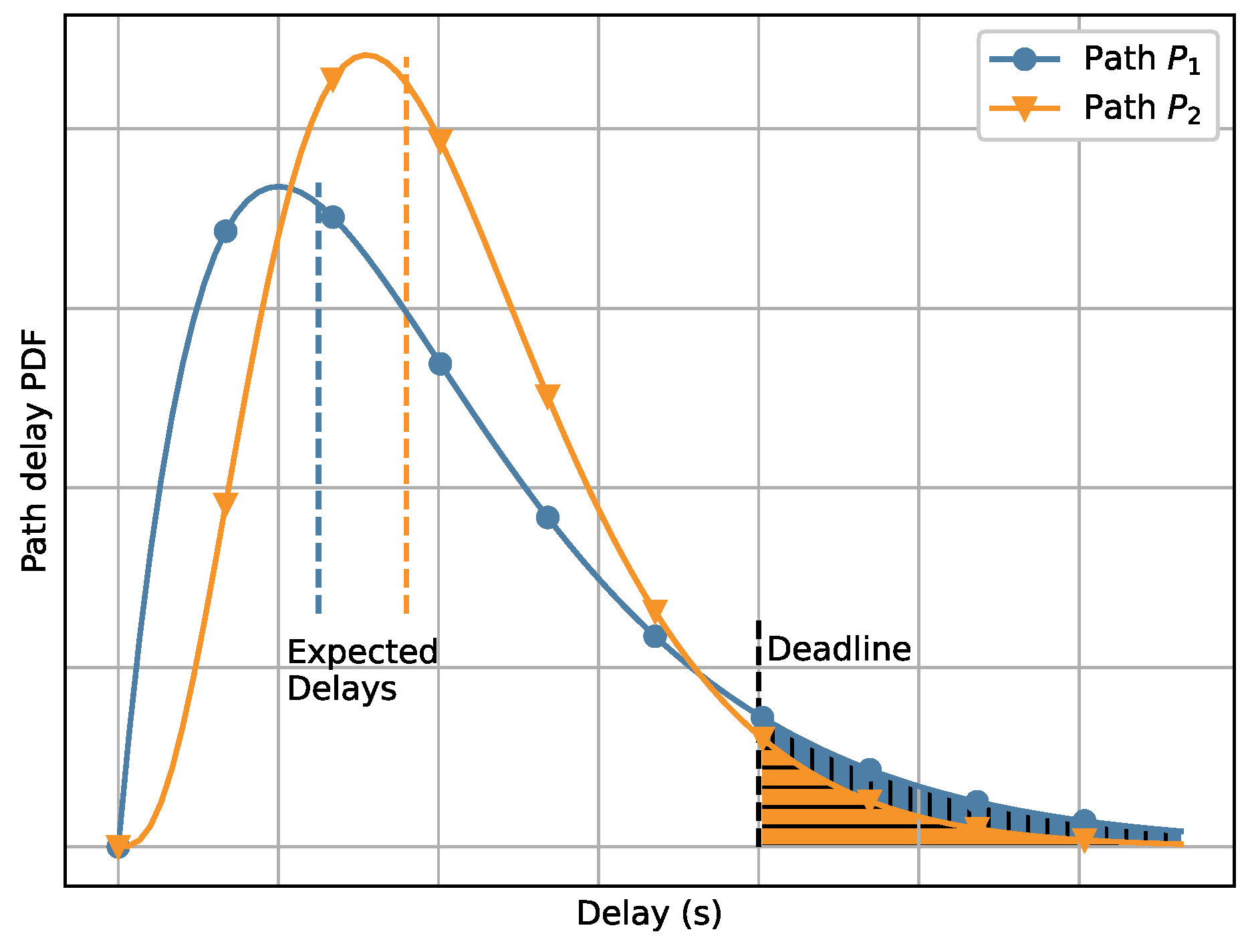
End-to-end (E2E) delay, which measures the time taken for packets to travel from a source node to a destination node in communication networks, is a widely used performance metric. It is frequently defined as the average delay of packets along a given path. This average delay is typically calculated as the sum of the average delays of each individual link along the path. However, it is crucial to point out that link delays possess inherent stochastic characteristics, leading to stochastic path delays and E2E delays within the network [1]. Consequently, link and path delays may be modeled by probability density functions (PDFs). An example is shown in Figure 1, which illustrates the PDFs of the delay of two paths and . The expected E2E delay of path (dashed orange line) is larger than the expected E2E delay of path (dashed blue line). By expected E2E delay, we refer to the expected value of the corresponding PDF.
Some existing and emerging wireless network communication applications in fields such as critical care and industrial processes require timely data delivery in order to fulfill their purpose. In these contexts, lost packets or missed deadlines can result in severe consequences, especially in industrial control applications [2]. Therefore, it is crucial to meet deadlines with a certain level of reliability. Analytic tools play a significant role in this context, as they can provide operators with key information about the supported delay and reliability bounds [3], helping operators to make informed decisions to fulfill the application’s requirements.
Consider thus a time-critical networking application requiring data from a source node to arrive at a destination node by a given deadline. In Figure 1, the deadline is shown by the dashed black line. The shaded areas under the curves to the right of the deadline indicate the probability of missing the deadline for each path. Even though path has a smaller expected delay than path , the probability of missing the deadline is higher along path . This example supports the idea that analyzing and designing time-critical network communications by considering the probability density functions of E2E delays rather than relying solely on statistical measures, such as expected delay, should be a beneficial approach.
![Jsan 13 00009 g001]()
Figure 1.
Two probability density functions of the E2E communication delay along two paths are shown. They differ in their expected delays (dashed lines) and their respective probabilities of missing a deadline (shaded area). Although the expected delay of path is lower than that of path , the deadline achievement probability of path is higher. Thus, minimizing the expected delay does not guarantee a maximized deadline achievement probability. Recreated from [4].

E2E delays ensue from the accumulation of delays of links followed by the data. We refer to the likelihood of successfully meeting a specified deadline for timely data delivery, considering the PDF of E2E delays, as the deadline achievement probability (DAP). Because the routing algorithm ultimately selects the paths, the statistics of E2E delays and the resulting DAPs are closely linked to the routing protocol in use.
Building on the aforementioned ideas, we present our first contribution in the form of an algorithm that determines the DAP between a source and a destination node based on probability distributions of link delays and the given routing tables. This algorithm allows for analyzing the DAPs of a wide range of routing protocols within the family of proactive, non-multipath or multicast routing strategies. This therefore contributes to works such as [5,6] by providing an additional methodology and corresponding performance metric for comparing routing protocols.
We further extend this algorithm to iteratively optimize the routing tables within the network, resulting in a routing protocol that maximizes the DAP for every transmitted packet. Both algorithms operate locally at each node and rely solely on information exchanged with direct neighbors. We prove the convergence of both algorithms to the correct solution within a finite number of iterations. In addition to these contributions, we present a practical implementation of the algorithm. We demonstrate its functionality through simulations and provide a quantitative assessment of its performance.
The structure of this paper is as follows. Section 2 provides an overview of related works in the literature. In Section 3, we formalize the problem of achieving deadlines using a mathematical model from operations research. The algorithm for determining the DAPs is developed in Section 4, and the algorithm for maximizing the DAP is presented in Section 5. The simulation set-up is provided in Section 6, followed by evaluation of the simulation results in Section 7. Finally, we conclude our findings in Section 9.
2. Related Work
In wireless networks with stochastic link characteristics, where link quality is subject to random variations, achieving deadlines becomes a complex task. A growing number of works have proposed paradigms and techniques to address these challenges and achieve deadlines in such conditions [7]. In the sequel, we highlight contributions relevant to this study. We will examine diverse techniques and protocols designed to enhance real-time capabilities in wireless networks, with a particular focus on the metrics essential for meeting deadlines.
In scenarios where the topology of the network and the links between nodes are subject to high dynamics or the routing layer has limited information about the network, approaches such as geographic routing (GR) can be particularly useful. Those conditions can be found in mobile ad hoc networks and wireless sensor networks (WSNs). GR leverages the geographic locations of nodes to make routing decisions, eliminating the requirement for explicit knowledge of the network topology. For deadline-aware traffic under this paradigm, velocities, understood as the speed or rate of movement of packets, are commonly utilized as a variable to support timely delivery. An early key contribution in this respect is the SPEED protocol [8], which proposes a GR approach with soft real-time guarantees and congestion avoidance for WSNs. Several extensions of SPEED have been proposed, including energy awareness [9,10] and packet prioritization combined with probabilistic multi-path forwarding [11]. Also, a combination of transmission power control and GR for improved energy efficiency was considered in [12]. In [13], the real-time routing problem is transformed into a 0/1 integer linear programming problem to effectively balance energy efficiency and reliability for real-time applications.
Predictive models can be employed to anticipate and adapt to future link variations. Reinforcement learning (RL) is a prevailing machine learning technique in the literature for routing. Unlike other machine learning techniques, it does not require large data sets [14]. RL provides a high level of adaptability, which allows the protocols to work in dynamically changing networks. Furthermore, RL approaches have been used to optimize for multiple criteria. For instance, Jafarzadeh et al. [15] proposed an energy-aware quality of service (QoS) routing protocol. In another study by Lin et al. [16], a joint optimization approach for routing and transmission power in dynamic environments was proposed, specifically targeting delay-sensitive applications.
Furthermore, various other techniques have been employed to enhance the performance of time-critical networking. For example, in [17], the authors proposed a routing mechanism for real-time communication in WSNs based on composite potential fields. The method, inspired by physics, models nodes as charged particles, and communication paths are determined by attractive and repulsive forces. The metric employed for decision making is the hop count, reflecting the number of intermediate nodes. Also, various cluster-based routing schemes have been proposed [18]. Cluster-based routing can be beneficial for time-critical applications as it optimizes communication by organizing nodes into clusters, reducing latency, enhancing reliability, and facilitating efficient coordination for timely data transmission. A cluster-based protocol for real-time traffic in industrial wireless sensor networks was presented in [19]. The protocol focuses on energy efficiency and reduced end-to-end delay. Real-time updates of routing information, focusing on geographical position, hop counts, and residual energy metrics, enhance overall system performance and scalability. Another cluster-based protocol, detailed in [20], caters to delay-sensitive, bandwidth-intensive, time-critical, and QoS-aware applications. It employs dedicated paths for real-time traffic, calculated using a metric that incorporates the initial energy, expected transmission count, inverse expected transmission count, and minimum loss.
Combinations of multiple approaches have also been proposed. For instance, opportunistic routing (OR) has been integrated with RL for live video streaming over multi-hop wireless networks [21]. Techniques from GR and OR have been combined in a QoS-aware scheme for wireless sensor networks [22]. Tang et al. [21] introduced a distributed RL-based OR scheme for video streaming, where a novel metric was proposed to estimate end-to-end (E2E) delays.
All of the above approaches focus on individual metrics, predominantly velocity or hop count, to ensure the timely delivery of data. However, the importance of modeling link latencies directly as probability distributions instead of using individual metrics has been highlighted in works such as [4,23].
Stochastic networks are characterized by aspects with uncertain behavior, and the parameters or conditions that affect network operations are subject to variability or randomness. Several works have considered deadline-aware routing for such networks. The reliable shortest path problem, introduced by Frank in [24], considers the joint latency of individual paths to select the optimal path for a specific deadline. While [24] is a contribution from operations research, the reliable shortest path problem has also received some attention in the domain of wireless multi-hop networks in works such as [4,23]. In contrast to the reliable shortest path problem, which focuses on predefined paths, the stochastic on-time arrival problem [25] allows for optimal decisions made on the fly. The stochastic on-time arrival problem has received little attention from researchers studying communication networks. It has been considered to provision soft QoS guarantees in mobile ad hoc multimedia networks [26] or for accomplishing timely data delivery in a practical bus network [27].
Routing algebra [28] can be used as a holistic mathematical modeling approach for designing and analyzing routing metrics. The key property of the algebra, isotonicity, is necessary and sufficient to prove that the routing produces loop-free paths. In [29], the authors extended the algebra to OR. Routing algebra can also be applied for combined metrics, such as a combination of a link quality indicator and the remaining energy [30]. In contrast, the optimal paths found by the atochastic on-time arrival problem may include loops [25]. This violates isotonicity, and therefore routing algebra is not sufficient to describe the stochastic on-time arrival problem.
Numerous studies have focused on the subject of deadline-aware routing in recent years, as indicated by our literature review. However, these works predominantly offer solutions grounded in either single or combined metrics. There is a clear absence of algorithms created through analytical methods that are based on the distribution of link delays.
In this paper, we use an analytical approach based on the stochastic on-time arrival problem in order to find the achievable deadline performance in communication networks and thereby provide a tool for the design of routing protocols that maximize the probability of achieving deadlines. We elaborate on this approach next.
3. Statistical Model for the DAP
Consider an ad hoc mesh network with data that must be relayed to a destination by a given deadline. In the sequel, we derive the process of calculating the DAP for each node in the network based on known routing tables for a given destination node. We begin with Section 3.1, providing detailed information about the probabilistic model of the delays of individual links and paths followed by packets. We then derive the DAP of a node in Section 3.2 using link delays and the E2E delay statistics of its neighboring nodes.
3.1. Link and DAP Statistics
Data packets are composed of application data and a deadline. For the deadline, we define the initial time to deadline (initial TTD) as a system-wide parameter. This represents the maximum allowable age for application data to arrive at the destination in order to be useful for the application. The deadline for the application data is therefore calculated by adding the initial TTD to the chronological time at which the data are passed down at their source to the network layer (NET) and the corresponding packet is formed. Subsequently, the node begins relaying the packet toward the destination. When a neighboring node receives the packet, its deadline is inspected. The packet is then routed with the aim of meeting its deadline.
Regardless of the trajectory followed toward the destination, each packet encounters numerous delays along the way. These are caused by transmission queues, channel access delays, retransmission timeouts, propagation delays, and protocol stack processing delays [31]. These delays are random with diverse statistics. We model the joint delay from the instant a packet is delivered to the NET of node u until it is successfully delivered one hop downstream to the NET of neighboring node by a random variable with PDF , with denoting the delay. Much work has been carried out to capture the link statistics (see, for example, the references in [32]). Because link delays are often dominated by path loss and channel fading, we assume that link PDFs are static and that link delays are random variables independent from each other.
As a packet moves toward its destination, realizations of the link delays add up over time, thereby reducing the remaining time to deadline (remaining TTD). The DAP of a packet en route depends on its remaining TTD (the shorter the remaining TTD, the lower the DAP). The cumulative distribution function that describes this relationship (DAP-CDF), seen from the NET, is denoted by , where u is the node to which the DAP-CDF pertains and is the remaining TTD.
Routing tables and DAP-CDFs are closely related. Any DAP-CDF can be determined by the method provided in [32]. However, it is to be noted that the corresponding algorithm in [32] requires complete and central knowledge of the link statistics and of the routing tables for the entire network. Our objective here is to find a distributed algorithm for each node to determine its DAP-CDF using only locally available knowledge. For this, a key observation is that the DAP-CDFs of neighboring nodes toward the destination are interdependent. We explore this interdependence in the following subsection and use it as the basis for our proposed algorithms.
3.2. DAP Relationship between Neighbors
Consider any network in which each node routes traffic based on deadline-aware routing tables, whose input is the remaining TTD of the packet to be forwarded and output is the next hop neighbor. Consider representing these routing tables by functions , which return the neighbor that node u chooses as next hop when the remaining TTD of a packet is . This representation encompasses many common cases. One particular case is when the forwarding node is the same neighbor regardless of the remaining TTD, such as in routing by the minimum hop count [33,34].
Assuming that the routing tables of all nodes in the network have been configured to a known and valid state, denoted as for any node u, we aim to determine the DAP for traffic originating from or passing through node u. To achieve this, assume that node u possesses the following statistics for each of its neighbors :
- (1)
- The PDF of the link delay from u to .
- (2)
- The DAP-CDF of corresponding to the routing tables set up in the network.
Then, the DAP-CDF seen from u when forwarding a packet via neighbor is given by the convolution of the above two probability functions:
In the above equation, denotes “forwarding from u via ”, and ∗ denotes the convolution operation. Given the routing table of node u, the DAP-CDF of node u for a remaining TTD satisfies the following equation:
In the next section, we provide an algorithmic description of how the DAP-CDFs can be determined in a distributed fashion for the entire network utilizing the insights discussed above.
4. Algorithm for Determining the Probabilities of Achieving Deadlines
Assume that the routing tables of all nodes in the network have been set to a known and valid state, for instance, by using a metric such as the hop count. The proposed algorithm for finding the DAP-CDFs corresponding to the routing tables is based on an iterative approach that leverages Equations (1) and (2). During iteration, intermediate cumulative distribution functions (CDFs) are obtained and denoted by . These CDFs eventually converge to actual DAP-CDFs, denoted by . The complete Algorithm for Determining the Probabilities of Achieving Deadlines (ADPAD) is presented in pseudo-code as Algorithm 1 below.
The algorithm has two phases: an initialization phase and a round-based updating phase of the node CDFs . Both phases run locally on each node and rely only on the exchange of information with direct neighbors. The algorithm description is therefore presented from the local view of an arbitrary node u. The algorithm is carried out in a distributed and joint fashion by all nodes in the network. No centralized processing is performed at any time.
The CDF of a given node u is initialized as (line 5). After initialization, a round-based updating of the CDFs begins. The destination s is an exception because its CDF is initialized as the step function ( for and 0 otherwise) (line 3) and does not ever change.
At the beginning of each new round, every node in the network and the destination broadcast their CDFs (line 9). We assume a mechanism is in place at the data link layer (DLL) for ensuring correct delivery to all corresponding neighbors. Upon receiving all neighbors’ CDFs (line 10), every node except the destination s performs one round of the algorithm. With a focus on node u, the round consists of the following two steps:
- Step 1:
- For every neighbor (line 11), node u calculates the expression in Equation (1), using the latest received instead of the still unknown (line 12). The set in line 11 denotes the neighboring nodes of node u in the network, consisting of the nodes to which u can directly communicate or forward data packets.
- Step 2:
- Node u updates its CDF according to Equation (2) (line 14). The resulting CDF will be broadcast at the beginning of the next round.
After performing the above steps, u waits until the beginning of the next round. The rounds are repeated at regular intervals by all nodes in the network.
| Algorithm 1 Algorithm for Determining the Probabilities of Achieving Deadlines (ADPAD) |
|
Appendix A presents proof that the ADPAD converges to a stable solution in finite time and that it returns actual DAP-CDFs. While DAP-CDFs obtained using the aforementioned approach correspond to given routing tables, it is important to note that these routing tables may not be optimal for deadline-aware traffic. A modification of the ADPAD can be made in order to also return DAP-optimal routing tables. The details of this modification will be explained in the following section.
5. Algorithm for Maximizing the Probabilities of Achieving Deadlines
Maximizing the DAP of network traffic requires that the forwarding decisions for each packet at each node are made with optimal deadline-aware routing tables given the remaining TTD. To iteratively improve the routing tables and ultimately maximize the DAPs, we introduce an additional step in ADPAD that involves updating the routing tables in each round. The resulting algorithm is presented as the Algorithm for Maximizing the Probabilities of Achieving Deadlines (AMPAD).
Empty routing tables are initialized in line 6. After finishing the loop in line 14, which calculates for all neighbors of node u, we carry out the following maximization in line 15, which may return a set with more than one optimal result:
Here, (without the check mark) represents the best routing choice(s) that node u can make for the remaining TTD based on its current knowledge about the network delays. In case the arg max operation provides more than one solution, must be chosen, for example, randomly from the returned set.
Let us assume that node u adopts a new routing table according to Equation (3). Then, the update of u’s CDF in line 14 corresponds to the newly adopted routing table. By recursively applying this to each round, the routing tables improve toward maximizing the DAP.
| Algorithm 2 Algorithm for Maximizing the Probabilities of Achieving Deadlines (AMPAD) |
|
The routing tables in the AMPAD are interdependent between nodes. Changes to one table may affect the DAP of neighboring nodes and therefore their tables, and so on, rippling this way through the entire network. Therefore, maximizing the DAP also yields the set of DAP-optimum routing tables for the entire network and not just for individual nodes. The proofs in Appendix A regarding convergence in finite time are also applicable to the AMPAD. Furthermore, we provide proof in Appendix B that the solution obtained by the AMPAD is optimal. This proof can be read in direct continuation of the proofs of Appendix A.
6. Simulation Implementation
We utilize WSNs as a use case for conducting simulations, although our algorithm can be applied to other network types as well.
The proposed algorithms were tested using Castalia [35], which is a simulator for WSNs based on the OMNeT++ platform. The algorithms were mostly implemented in the NET. We kept the other layers of the protocol stack as standard as possible. A brief description of all relevant layers and processes is presented below.
6.1. Wireless Channel Model
The wireless propagation medium was simulated using a lognormal shadowing model with an exponent of , a reference distance of 1 to the far field of the antennas, and a path loss of at that distance. A lognormal random shadow fading with a standard deviation of 4 was generated for every link. Additionally, quasi-static Ricean fading with a K factor of four was employed to simulate small-scale block fading, a value found in many different environments.
6.2. Physical Layer (PHY)
The physical layer (PHY) used was the one corresponding to the CC2420 chipset, with default values as implemented in Castalia. The chosen modulation type was “Ideal” with a signal-to-noise ratio threshold of 5 for successful reception. The transmit power was set to 0 .
6.3. Data Link Layer (DLL)
The MAC protocol was implemented as a standard unslotted, non-persistent carrier-sense multiple access (CSMA) protocol with acknowledged connectionless service. The implementation of Timeout-MAC [36] in Castalia served as the basis for implementing this protocol. Retransmissions are carried out after 5 in case no acknowledgment is received. Acknowledgments are transmitted immediately after the frame to be acknowledged is received, while all other nodes hold contention. After two transmission attempts without successful reception of an acknowledgment by the sender, the frame (packet) is discarded.
Link delay estimations were implemented in the DLL. For this, a timestamp is noted when data packets or probing packets are passed from the NET to the DLL and queued at the MAC. Once the sender receives an acknowledgment, it estimates the delay to the receiver by calculating the difference between the acknowledgment’s reception time and the initially noted timestamp, subtracting the air time of the acknowledgment frame. The measured delay is then forwarded to the NET for maintaining link delay statistics.
Acknowledgments also include a flag to indicate if a frame has already been received and acknowledged before. If the flag is set, then prior ACKs got lost, and the actual delay experienced by the packet for reaching the neighbor was shorter. In these cases, the acknowledgment is not used for link delay statistics.
6.4. Network Layer (NET)
When a packet becomes available at the NET for transmission, the deadline-aware routing table is looked up, and the packet is passed down to the DLL. Generating adequate routing tables in the simulator relies on three key processes at the NET: estimation of the link delay PDFs, the exchange of CDFs between neighbors, and a mechanism for avoiding the “count to infinity problem”. Each process is described below.
Estimation of link PDFs: Both proposed algorithms require knowledge of the probability distributions of the link delays seen at the NET between neighbors (see Equation (1)). Because, in practice, these PDFs are unknown a priori, they must be estimated and updated regularly. For this, link delays are measured (1) actively by means of probing packets and (2) passively by harvesting delay information from transmitted data packets. Probing packets are unicast by each node to all their neighbors every 120 .
Link delays observed by the DLL are stored as histograms at the NET. The histograms consist of 101 bins, where the first 100 bins are uniformly distributed for times from 0 to the initial TTD. Bin 101 counts the number of observed delays above that time, including the count of packets discarded at the DLL.
The link delay PDFs are determined by dividing the number of measured delays in each bin by the total number of measured delays. This quotient is then multiplied by the packet delivery ratio of the respective link.
Exchange of CDFs among neighbors: The two proposed algorithms require a regular exchange of DAP-CDFs between neighboring nodes. For this, the broadcasting of CDFs is performed at regular intervals of 5 s.
Preventing the “count to infinity problem”: We have observed for both algorithms that the DAP-CDFs are slow to incorporate evolving link statistics. As a consequence, the exchanged DAP-CDFs may provide an inaccurate snapshot of the network’s actual link statistics. With the ADPAD, this simply delays its convergence. However, for the AMPAD, it may lead to routing loops in a similar fashion to the “count to infinity problem” of distance vector routing (Section 5.2.4 in [37]). In order to avoid this effect and avoid routing loops, we propose using a solution based on an aging sequence number, whereby every node starts with a sequence number with a value of zero and attaches it to every transmission of DAP-CDFs. The destination node increments its own sequence number every 120 . This increment propagates through the network in a flooding fashion when the DAP-CDFs are exchanged. Each time a node receives a new DAP-CDF from a neighbor, it inspects the enclosed sequence number. If it is larger than its own sequence number, then the following processess are carried out:
- The node’s own sequence number is updated to the newly received sequence number.
- A new empty routing table (“scratch table”) is allocated (but not yet used). This table will be updated several times by the steps explained below. It will become operational (i.e., used for forwarding decisions) the next time it receives a sequence number greater than its own (when these steps are applied the next time and a new scratch table is allocated).
- All locally stored DAP-CDFs of the neighbors are erased.
- All link PDFs are calculated from the current histograms.
In the previous case, and in case the received sequence number is equal to the node’s own number, the DAP-CDF is updated locally according to lines 12–14 and 16 of Algorithm 2. The scratch table is updated every time according to line 15.
Finally, when the received sequence number is smaller than the node’s own sequence number, then the received DAP-CDF is considered outdated and ignored.
6.5. Transport Layer
Because application data are embedded in individual packets that fit inside single transmission frames, and because transport control protocols entail long sink-to-source feedback loops, we opted not to implement any form of transport control.
6.6. Application Layer (APP)
In our simulation, the application layer (APP) laid right above the NET. It produced data units of 10 bytes in size which needed to be delivered to a sink node within an initial TTD that was set for all nodes equally, ranging from 12 to 100 in the various simulation runs. Data units were generated at each node at a rate of one unit every 80 .
6.7. Benchmarking Protocols
The DAP performance obtained with the AMPAD was compared to the DAP of distance vector routing (Section 5.2.4 in [37]) based on three common and widely used metrics [6,7].
The average delay (AD) aims at minimizing the average delay of packet deliveries. Considering the delay experienced along different paths, the routing algorithm can dynamically adjust routing decisions to steer traffic away from congested links or nodes.
The hop count (HOP) routes packets by minimizing the number of hops used to reach the destination node. This routing method is relatively simple to implement and requires minimal computational resources compared with other routing algorithms. Its low overhead is particularly attractive for energy-constrained wireless mesh networks.
The expected transmission count (ETX) [38] selects the path with the lowest expected number of transmissions from a source to a destination. By considering the link quality, links with poor performance are avoided and packets are routed through paths with higher link quality, reducing the energy consumption associated with retransmissions.
The implementation of these routing alternatives is identical to the protocol used for the AMPAD, with the only difference being that, instead of determining probability density functions (PDFs) and exchanging the corresponding cumulative distribution functions (DAP-CDFs), only the values of the respective metrics are estimated and exchanged. Forwarding decisions are made by choosing the neighbor with the minimum metric value to the destination node. The “count to infinity problem” is avoided using the same method based on sequence numbers described in Section 3.1.
Note that for all comparison metrics, a node’s neighbors are defined as the nodes whose packet loss rate, seen at the NET, is below a certain threshold. This enables the examination of the effects caused by lossy links.
6.8. Network Realizations
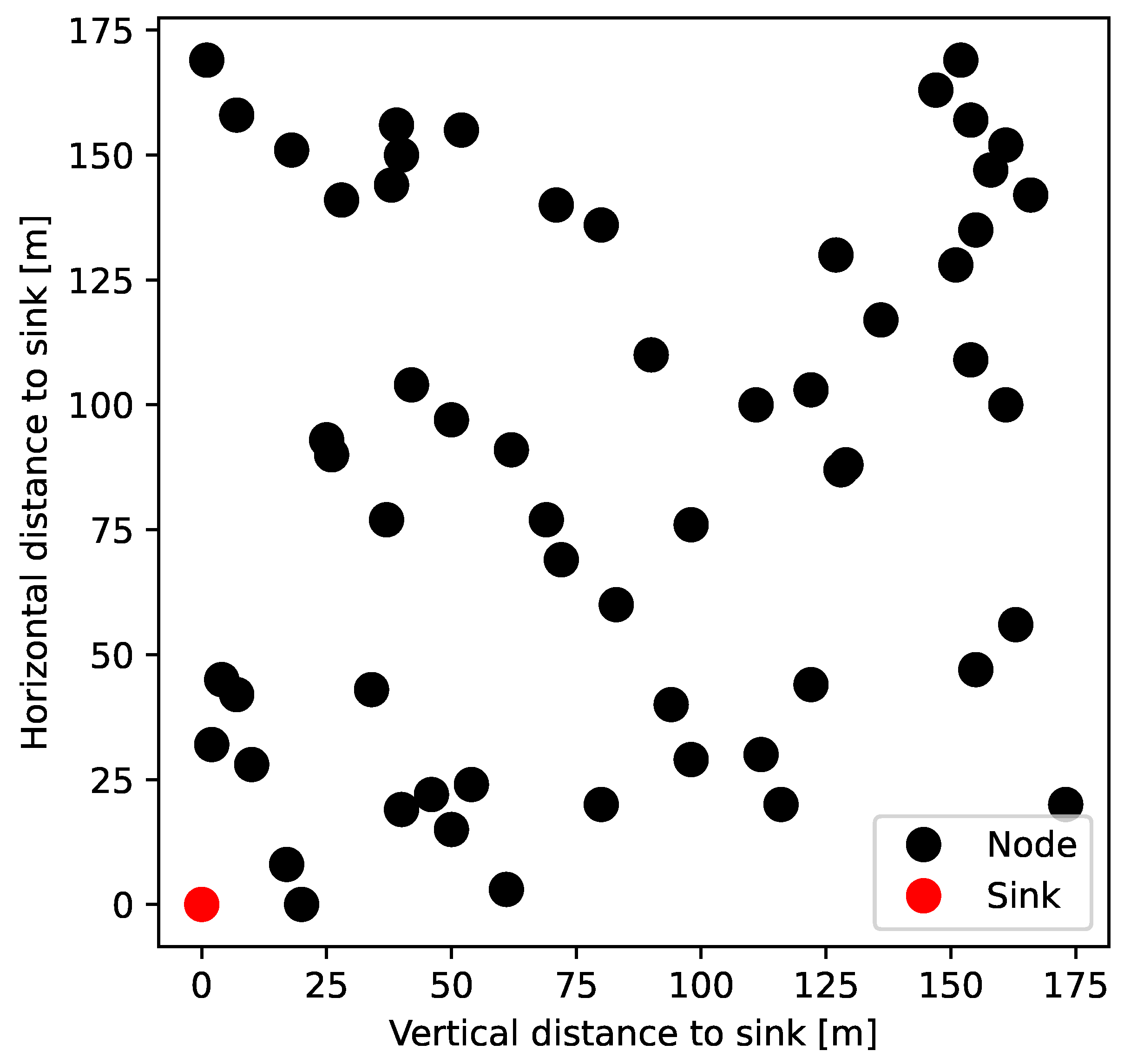
In the context of our WSN example, we assumed a dedicated network tailored for a specific purpose. Consequently, the entirety of network traffic comprised exclusively time-critical data packets and packets containing routing information. Most simulations were performed with mesh networks of 60 nodes placed randomly with a uniform distribution on a square area of 30,000 , as shown in Figure 2. The sink was placed in the southwest corner, and 60 networks were generated this way and used for all reported results.
Line topologies are sometimes found in real WSN deployments [39], such as those involved in monitoring gas pipelines [40]. These simpler topologies enable a focused examination of the behaviors exhibited by the protocols under study. Two experiment sets were carried out in a line topology, with 60 nodes placed at a distance of 5 from each other and covering a total distance of 295 . In this case, simulations were repeated 60 times with different seeds.
All simulation parameters and their default values are shown in Table 1.
7. Performance Evaluation
In this section, we evaluate the performance of both proposed algorithms via simulation.
The first batch of simulations was run to validate that the ADPAD and AMPAD produced accurate DAP-CDF estimations. The evaluation was performed with the AMPAD because the ADPAD does not have a priori defined routing tables, while the AMPAD determines them. Whether these are optimal or not in the DAP sense is not relevant in this case.
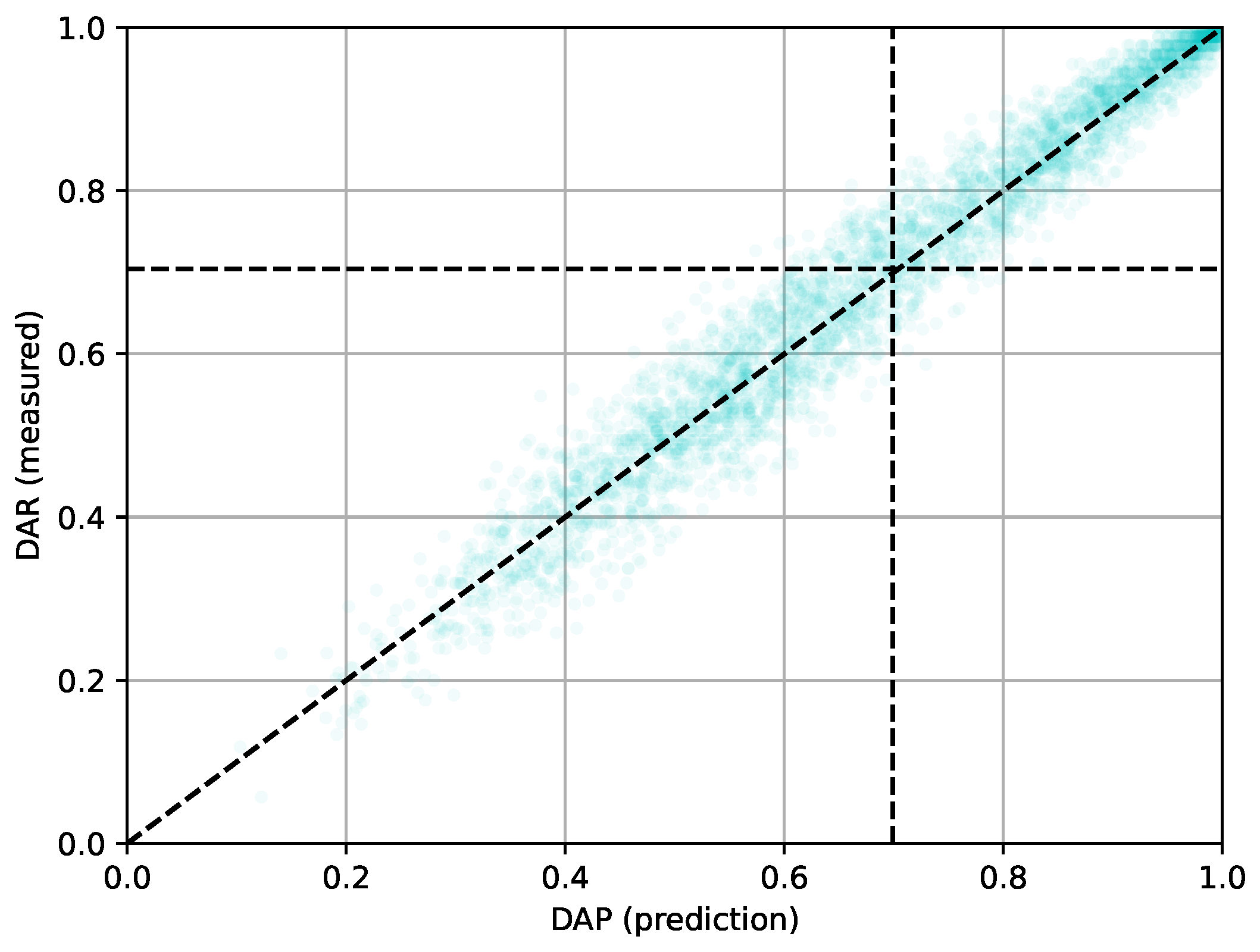
The simulations recreated 32 h of network time, of which the last 8 h were used for measuring the actual deadline achievement ratio (DAR) of the data packets. The DAR is the fraction of data packets created in the network that arrive at the sink within their respective deadlines. During the simulation, certain packets were lost for reasons such as channel access failure or reaching the maximum number of transmission attempts. We also classified such occurrences as instances of missed deadlines. Figure 3 compares the measured DAR values with the DAP predicted by the DAP-CDFs that were reached by the AMPAD at the end of the simulations. In all cases, the initial TTD was 35 . The DAPs versus DARs of all 3600 nodes of all 60 simulation runs of the square topologies are plotted in the figure. The DAP is overestimated above the diagonal dashed line; below the line, it is underestimated. The dashed horizontal and vertical lines represent the respective average values. The mean square error of DAP prediction versus the actual DAR was . This confirms that the algorithm converged to the correct DAP-CDFs.
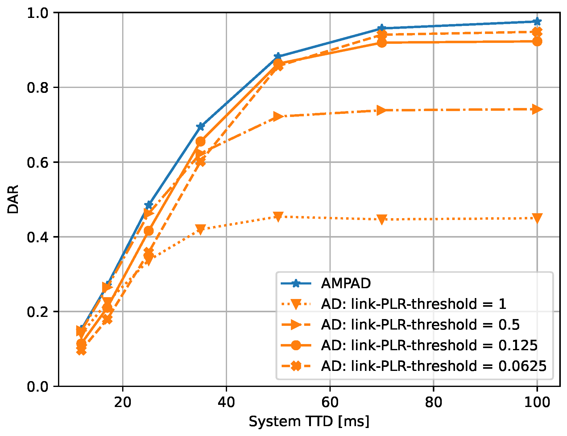
Next, we are interested in understanding the role of the link quality in the performance of the algorithms. The motivation for studying this aspect is as follows. Links with a longer physical distance tend to have a higher outage probability. On the other hand, long links move packets potentially faster toward the sink because fewer hops are needed. When the initial TTD is small, we expect better DAR performance when links with a higher packet loss are allowed because that enables using fewer hops to the sink by following longer and less reliable links. When a longer initial TTD is specified, then using links with lower packet loss is beneficial because that fosters the use of shorter, more reliable links when more hops to the sink are tolerable. We are interested in understanding how well the AMPAD deals with this trade-off in comparison with AD. For this, we used the loss rates of packets at the data link layer seen by the network layer (link-PLR) for ruling out links with poor performance in AD while keeping all links available to the AMPAD.
The following thresholds for the maximum allowable link-PLR for AD were tested: , , , and 1. A link-PLR-threshold of one does not impose any constraints on the neighbors that can be chosen for routing. In this case, the next hop selection was based only on the average times, regardless of packet loss.
The AMPAD and AD were simulated with the described square network realizations, with the various link-PLR thresholds for AD and varying initial TTDs. The performance metric of interest is the achieved DAR, which was averaged over all nodes and all simulated networks. The results are plotted in Figure 4. As expected, the DAR benefited from larger initial TTDs in all cases. The AMPAD consistently achieved the highest DAR performance for all initial TTDs. Interestingly, the DAR did not tend toward one in all cases, even with a large initial TTD. This is because the DLL discards frames that fail to reach the next hop neighbor within the given maximum number of allowed transmission attempts. This cause of packet loss is substantial for AD with thresholds that allow more unreliable links to be used. It drops as links with high link-PLR are filtered out through the thresholding method described. The curves for AD reflect the trade-off between the link length and hop count as the initial TTD varied. The ideal link-PLR threshold depended on the initial TTD; high link-PLR thresholds were better for low initial TTDs, and low link-PLR thresholds were preferred for high initial TTDs. The effect of lowering the link-PLR threshold for keeping better quality links had a limit because it reduced network connectivity, eventually creating isolated nodes or network islands whose traffic could never reach the sink, thus deteriorating the DAR further. Similar behavior was observed in the case of the other metrics, HOP and ETX, when different link-PLR thresholds were applied (not shown). It is to be noted that the AMPAD is free from this trading off by thresholding the link quality. It picks the optimal links automatically.
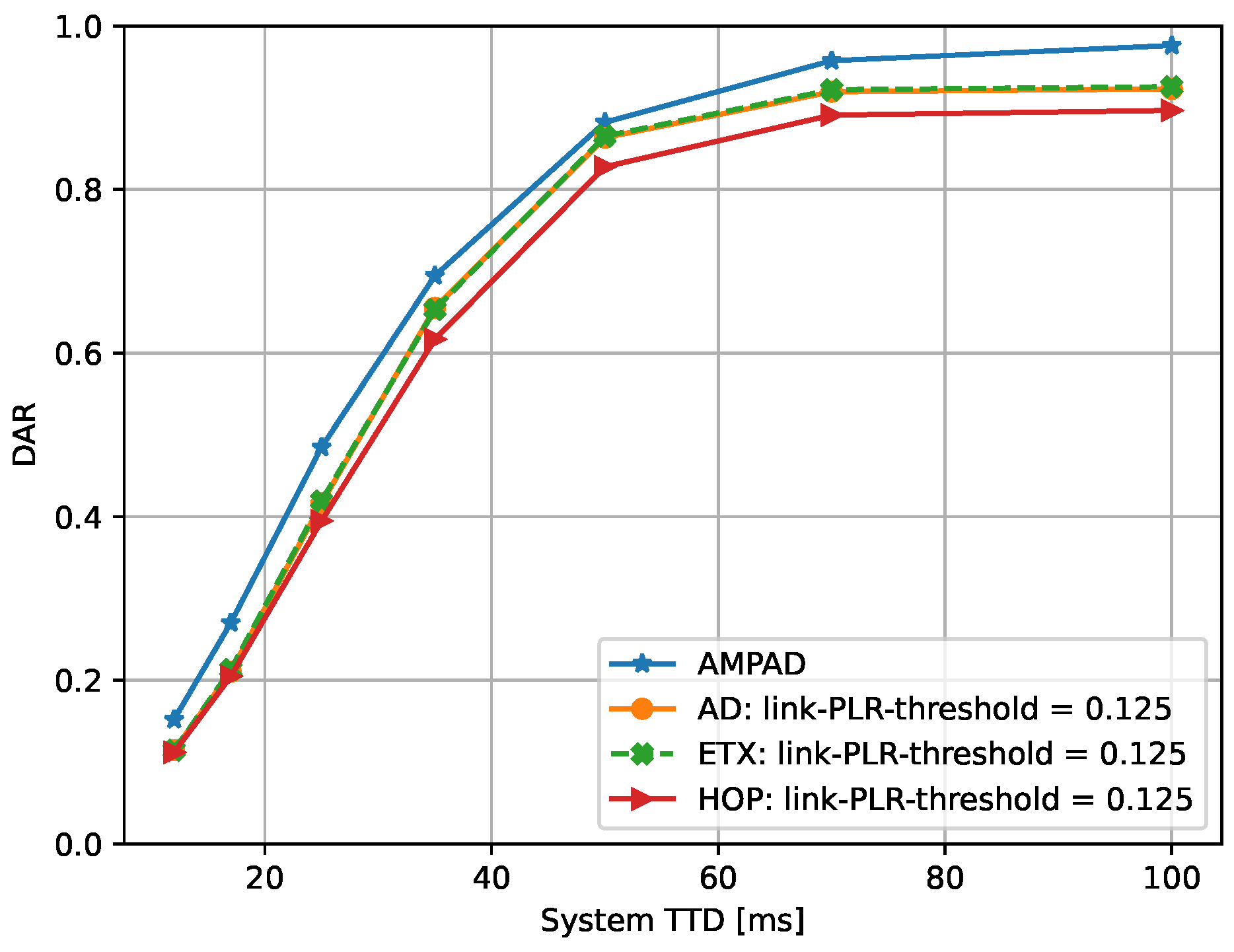
Next, we assessed the performance of the various routing algorithms for different initial TTD values with a link-PLR threshold of for all approaches (except the AMPAD). The results are shown in Figure 5, which presents the average DAR statistics from 60 simulation runs with the square topology with 60 nodes each. The variance in DAR values producing those averages (markers) was generally wide, including nodes close to the sink with DAR values close to one and nodes far away from the sink with DAR values close to zero. The AMPAD had the highest DAR among all considered initial TTD values, consistently outperforming all other approaches. On the other hand, HOP consistently exhibited the poorest performance out of all the algorithms simulated, while ETX and AD performed slightly better and similarly between them.
Next, we considered a line topology of 60 nodes distributed evenly over a distance of 295 , with the sink located at one end of the line. Based on empirical observations, we opted for a consistent initial TTD of 35 throughout all simulation runs. This specific initial TTD choice was deliberate to present a challenging scenario for the protocols, allowing for a thorough analysis of their behaviors across all nodes in the network.
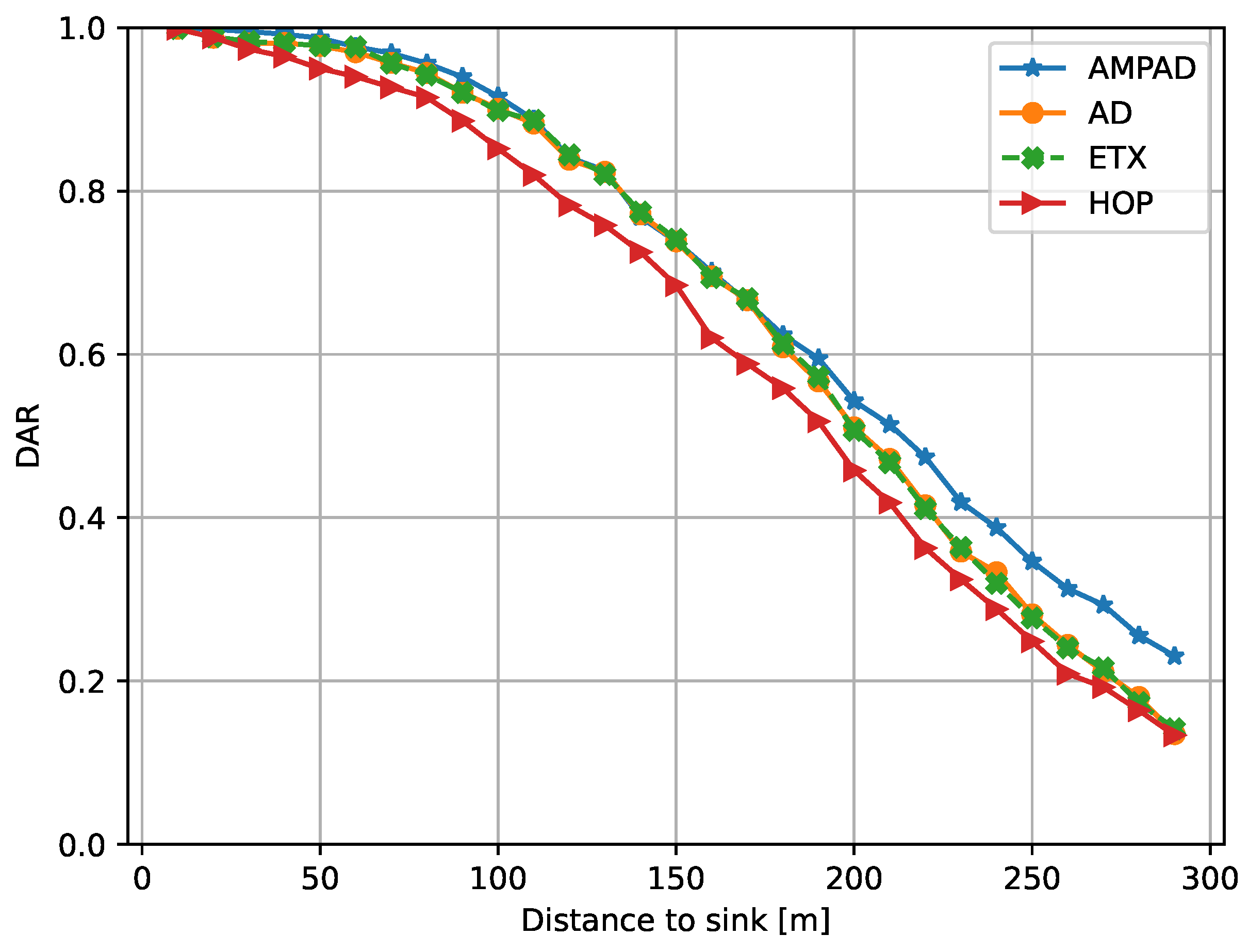
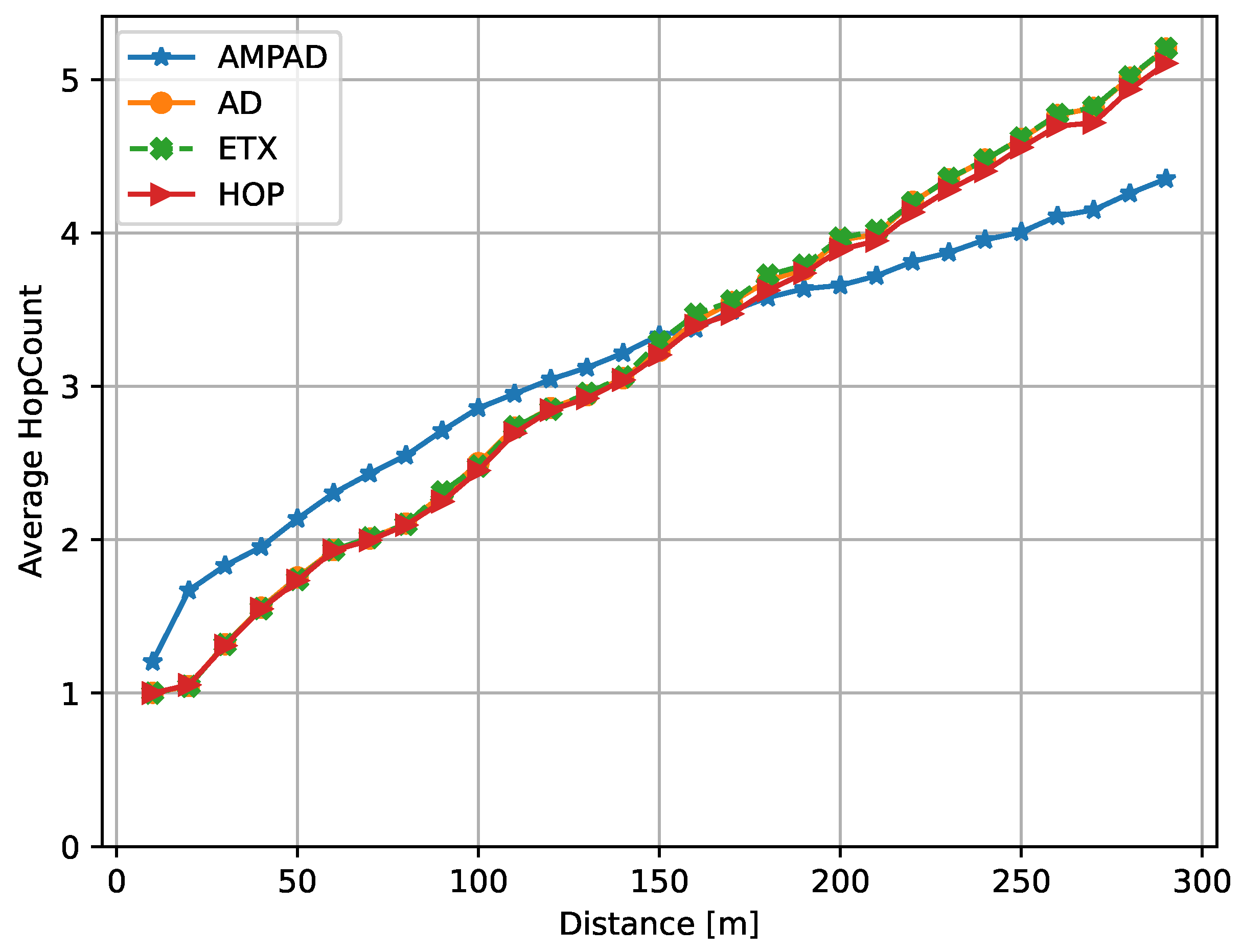
It is intuitive that the DAR dropped with an increasing distance to the sink because data packets originating from nodes located further away from the sink would follow longer paths (more hops). Figure 6 depicts this relationship between the distance to the sink and DAR, while Figure 7 presents the average hop count as a function of the distance for packets that successfully reached the sink within their deadline. Intuitively, for nodes at a high distance from the sink, priority should be given to fast paths rather than reliable ones. Conversely, at shorter distances, deadlines can be achieved by following slower but more reliable links and paths. This trade-off was observed for the AMPAD (Figure 7) but not for the benchmark protocols, whose hop counts increased approximately proportionally to the distance to the sink. With the AMPAD, nodes in close proximity to the sink (below 150 ) tended to utilize paths with higher hop counts compared with the benchmark protocols, resulting in improved reliability. Conversely, nodes located further away from the sink (above 170 ) tended to utilize paths with lower hop counts compared with the benchmark protocols, leading to reduced latency. This explains the superior DAR performance of the AMPAD shown in Figure 6 for short and long distances.
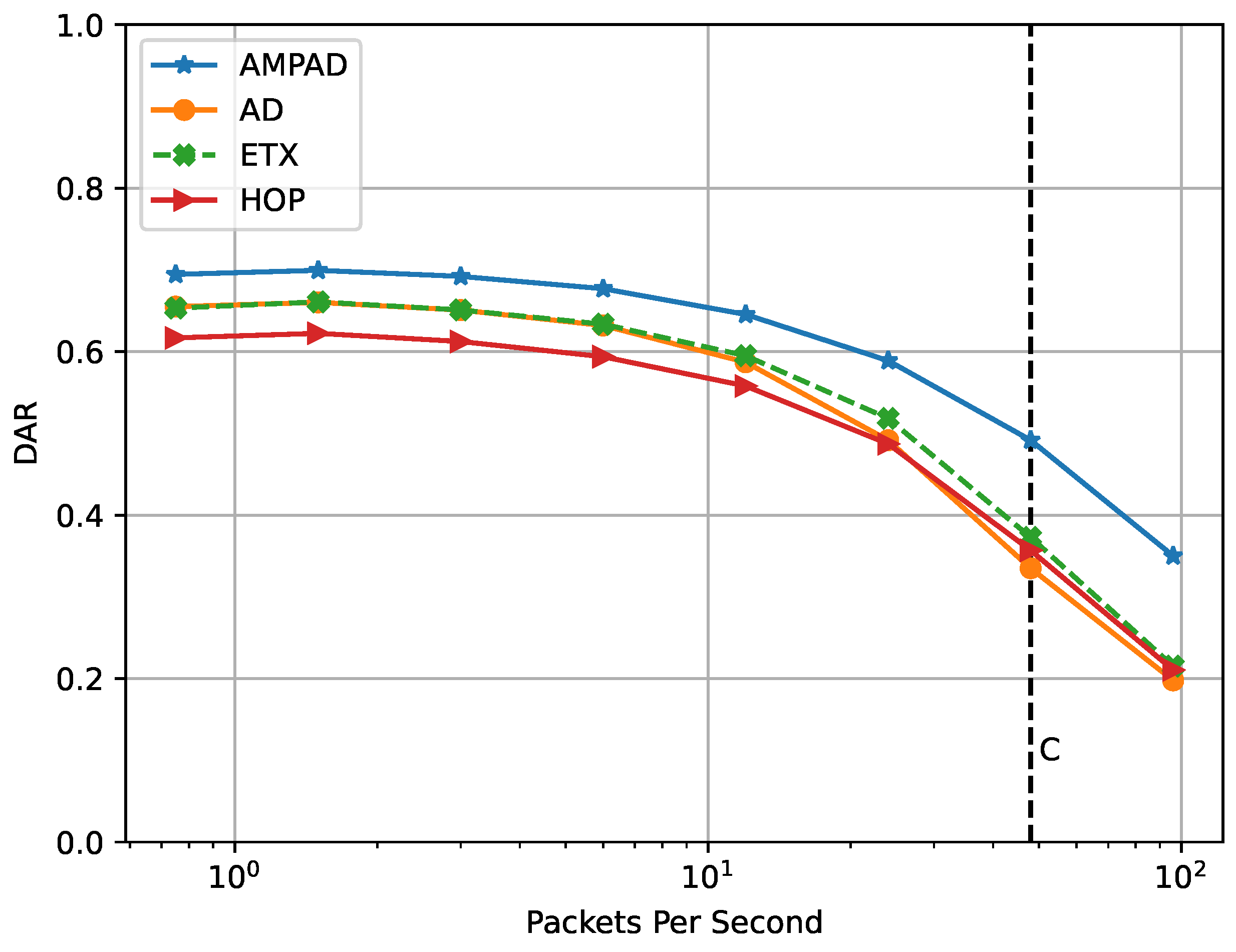
In Figure 8, we show the performance of the different approaches in terms of the DAR under various constant traffic loads in the square networks with 60 nodes and an initial TTD of 35 . Traffic ranged from to 96 packets per second and was generated at the application layer. The AMPAD consistently outperformed the other approaches, with a DAR difference of up to under high traffic conditions. The superior performance of the AMPAD was partly a result of how the AMPAD discards packets; it does so before the deadlines have passed and as soon as the deadline achievement probability reaches zero, while the other approaches discard packets only after their deadlines have passed. Consequently, traffic load was alleviated sooner under the AMPAD, especially near the sink, where traffic load was the highest. As a result, the AMPAD was able to maintain a more robust performance under high-traffic scenarios compared with the other approaches.
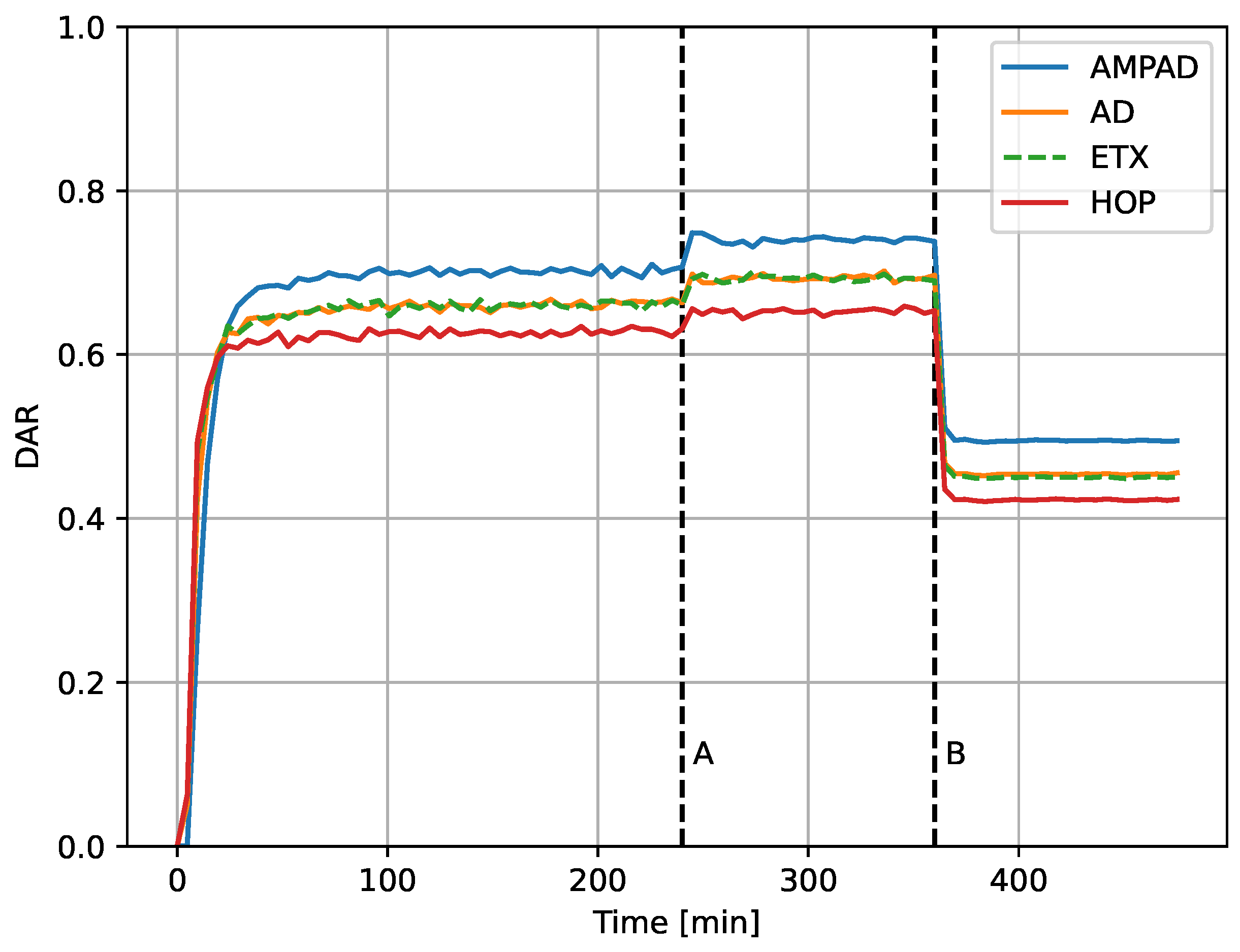
Figure 9 presents the performance of the different approaches over 8 h of simulation time under varying traffic load. The traffic load was set initially to packets per second for the first 6 h (left of line B) and then increased to 48 packets per second for the remaining 2 h. At 4 h (line A), all overhead traffic at the NET (link probing and broadcasting of CDFs, etc.), as well as updating of the routing tables, was stopped for the remaining simulation time. The DAP slightly improved at this time because of the freed up network bandwidth. At 6 h (line B), the figure depicts a decline in performance because of the traffic burst. The protocols continued to rely on previously established routing tables set up from DAP-CDFs and metrics that corresponded to the initial load conditions.
When comparing the performance during the last 2 h of network time in Figure 9 (48 packets per second to the right of line B) with Figure 8 at that traffic load (line C), it stands out that the AD, ETX, and HOP performed better in the burst case (achieving DAR values above compared with values below it). This was due to the additional bandwidth for lack of monitoring overhead. In contrast, the AMPAD achieved similar performance in both experiment sets. This indicates that the added bandwidth was lost for the suboptimal routing tables. Nevertheless, the AMPAD still outperformed all other approaches.
The frequency of retransmission attempts and packet loss rates at the DLL were strongly influenced by small-scale fading in the wireless propagation medium. In Figure 10, we investigated the performance of the AMPAD under various values of the Ricean fading K factor and compared it to the benchmark protocols for an initial TTD of 35 .
We observed that all cases performed worse at smaller values of K, confirming that networks with stronger small-scale fading in their links present more challenging routing environments for time-sensitive traffic. This highlights the importance of studying networking protocols under different fading conditions. Notably, the AMPAD exhibited an approximately higher DAR performance compared with the other approaches under intensive fading conditions (). At high K values (reliable links), both the AD and ETX demonstrated comparable performance to the AMPAD, while the HOP exhibited inferior behavior. Hence, one of the strengths of the AMPAD is its versatility in coping with different fading conditions.
8. Considerations for Energy Consumption
The optimization of energy consumption was not addressed in this study. However, in the domain of WSNs, energy consumption can be of paramount importance. In the sequel, we discuss aspects of our solution that contribute to the topic of energy consumption. Given that our protocol operates on probability density functions, in contrast to conventional protocols, an increased energy expenditure is anticipated. This can be attributed, on one hand, to the more intricate calculations and, on the other hand, to the larger packets required for transmitting routing information. Additionally, probes are employed for monitoring individual links, contributing to higher energy consumption.
However, the protocol effectively mitigates energy consumption by promptly discarding packets that are unable to meet their deadlines, thereby improving the overall energy balance. Additionally, passive monitoring contributes to reduced energy consumption. In situations where data traffic is high in relation to the routing overhead, the positive energy effects of our presented protocol may outweigh the associated costs. This remains an open topic for future analysis.
Nevertheless, for deployment in energy-constrained scenarios, an optimization focusing on energy is crucial. The probability functions employed in our approach allow integration with additional metrics that could be leveraged to reduce energy consumption or achieve a more balanced load distribution. Furthermore, it is conceivable to apply the proposed approach to exploit different transmission rates and performance levels in order to select the most energy-effective option for meeting a given deadline. Optimization strategies for energy efficiency should be explored for practical applications in resource-constrained environments.
9. Conclusions
Maximizing the probability of achieving E2E communication delay deadlines in communication networks was studied. The deadline achievement probability for given routing tables was derived.
We introduced a distributed iterative algorithm that finds the E2E delay cumulative probability functions. The algorithm was extended to also converge to optimal routing tables that maximized the probability for all packets to fulfill their deadlines. Both algorithms were proven to achieve a solution in a finite number of iterations. A solution was proposed that avoids the algorithms running into the “count to infinity problem”.
The simulation results show the proposed algorithms converging to the correct cumulative distribution functions of the deadline achievement probabilities for all nodes in a network.
The deadline achievement ratio of the proposed algorithm with routing table optimization was benchmarked against the performance of routing by different common metrics (hop count, average delay, and ETX). The latter were tested, ruling out poor quality links using various thresholds for link packet loss ratios. It was shown that the proposed approach consistently outperformed the other routing metrics, regardless of the threshold used. Notably, the AMPAD exhibited an approximately higher DAR performance compared with other approaches under intensive fading conditions ().
We further found that the proposed approach is versatile for coping with small-scale channel fading and varying traffic loads. Under strong fading conditions, our approach demonstrated a roughly higher deadline achievement ratio compared with the benchmark protocols, with no significant performance improvement observed under mild fading conditions. Additionally, across varying traffic loads, our approach outperformed the benchmark protocols by up to .
Deadline-aware routing using link statistics is a promising approach, especially for severe channel fading conditions.
Author Contributions
Conceptualization, C.O., B.B. and T.M.; methodology, C.O. and B.B.; software, B.B.; validation, C.O., B.B. and T.M.; formal analysis, B.B.; investigation, C.O. and B.B.; resources, R.S., C.O., B.B. and T.M.; data curation, C.O. and B.B.; writing—original draft preparation, C.O. and B.B.; writing—review and editing, R.S., C.O., B.B. and T.M.; visualization, C.O. and B.B.; supervision, R.S. and T.M.; project administration, C.O. and T.M.; funding acquisition, R.S., C.O. and B.B. All authors have read and agreed to the published version of the manuscript.
Funding
This work was supported in Chile by the Research Center for Integrated Disaster Risk Management (CIGIDEN), Proyecto 1522A0005 FONDAP 2022, the German Research Foundation (DFG) within the Collaborative Research Center (CRC) 1053 MAKI, and the LOEWE initiative (Hessen, Germany) within the emergenCITY center.
Data Availability Statement
The software presented in this study is openly available in the GitHub code repository (Benjamin Becker TUDa, Maximizing the Probability of Achieving Deadlines, 2024).
Conflicts of Interest
The authors declare no conflict of interest.
Abbreviations
The following abbreviations are used in this manuscript:
| AD | Average delay |
| APP | Application layer |
| ADPAD | Algorithm for Determining the Probabilities of Achieving Deadlines |
| AMPAD | Algorithm for Maximizing the Probabilities of Achieving Deadlines |
| CDF | Cumulative distribution function |
| DAP | Deadline achievement probability |
| DAR | Deadline achievement ratio |
| DLL | Data link layer |
| E2E | End-to-end |
| ETX | Expected transmission count |
| GR | Geographic routing |
| HOP | Hop count |
| Link-PLR | Loss rates of packets at the data link layer seen by the network layer |
| NET | Network layer |
| Probability density function | |
| PHY | Physical layer |
| QoS | Quality of service |
| RL | Reinforcement learning |
| TTD | Time to deadline |
| WSN | Wireless sensor network |
Appendix A. Proof of Convergence to a Stable Solution for DAP-CDFs
The proof is broken up into three parts. First, we show that the algorithm makes progress in each round toward the stable solution (Proof 1). Second, it reaches the stable solution after a finite amount of time (Proof 2). Third, the stable solution found by the algorithm returns proper DAP-CDFs (Proof 3).
The proofs that follow are valid for the AMPAD and ADPAD but are developed for the broader case of the AMPAD.
Appendix A.1. Proof 1: Steady Progress
Consider an approach based on induction using an integer index r, whose initial value is zero and is incremented on each round after completing a CDF exchange by the broadcasting in line 11 of the AMPAD. For the proof, we denote the resulting CDF by , which is initialized as (except for the sink, as noted). Similarly, we define
for for representing the CDFs calculated at round r (AMPAD, line 13). It is to be noted, however, that index r is used exclusively for clarity of the proof, but the nodes themselves do not use it nor know it.
Assume that all links exhibit a minimum link delay for any data packet transfer. Concretely, no link can transfer data packets with zero delay. This implies a delay below which all link PDFs are always equal to zero. Formally, by defining E as the set of all links in the network
then using r, we define the stable region for a CDF as follows:
where is a round-dependent variable whose initial value at is . The initial stable region of all CDFs is therefore, trivially, the set of negative real numbers.
Next, we show that the stable region of the CDFs grows with r and is lower bounded by .
Lemma A1.
is stable for .
Proof.
We will prove this lemma by induction. The induction basis for is trivial to show. For the induction step, we will show now that is stable for using the assumption that is stable for .
At the beginning of round , each node knows the CDFs of all its neighbors from the previous round. This is also true in particular during the first calculation of lines 12–16 of the ADPAD when and each node has just received the broadcast of the initial CDFs .
We first show that the CDF for any neighbor is stable for under the given assumptions. The following sequence of equations starts by considering these values of for :
Equation (A6) is the definition of taken from Equation (A1). Equation (A7) is then the common definition of convolution. The second summand in Equation (A8) is equal to zero according to Equation (A2), which leads to Equation (A9).
We now have to verify that all used values in the CDF are stable in Equation (A9). The considered values of t in are smaller than and are therefore stable by assumption. The link PDF is always stable. The stability of Equation (A9) proves the stability of for .
For each neighbor of u, the node u will update its own CDF (ADPAD line 16). Because every single value used to determine is the maximum among CDFs , the stable interval applies for . □
It follows from Lemma A1 that at the end of round , the stable region has grown to at least for all CDFs in the network. In general, when a node calculates for each neighbor and updates its own CDF (ADPAD, lines 12–16), the stable interval grows to at least . Hence, the stable interval grows with each new round. For the particular case of the AMPAD, it is to be noted that the stable interval found for all CDFs after completion of round r also implies that the routing tables of all nodes in the network are stable for delays up to at least as well.
The question is whether there is a finite number of rounds after which no CDF and hence no routing table can change anymore, therefore reaching a stable solution and establishing permanent CDFs and routing tables. This aspect is shown next.
Appendix A.2. Proof 2: Stability Reached in Finite Time
We wish to show that there is a value for r from which on the CDFs no longer change with increasing r values. For this, assume that every link has a maximum delay for which delivery to the corresponding neighbor is guaranteed. This implies that all link PDFs satisfy the following condition:
Next, note that in a connected network, at least one path from any given node u to the sink must have a finite number of hops. The deadline achievement probability PDF following that path is given by the convolution of all the link PDFs along the path. If the path has n hops, then by Equation (A10) and the properties of the convolution, it is guaranteed that the DAP-CDF of u is equal to 1 . Therefore, for all r such that , the CDFs must be stable over their entire domain of .
Considering the above fact for all nodes in the network, it is apparent that all DAP-CDFs eventually reach a stable state. The number of rounds needed to achieve stability is at most , with being the number of hops of the longest considered path in the network. This finishes the proof of convergence to a stable solution.
Appendix A.3. Proof 3: Algorithm Returns Actual DAP-CDFs
The AMPAD was shown to reach a stable solution for the functions in finite time. However, it has not been shown that these functions are proper CDFs of the deadline achievement probabilities (DAP-CDFs). This aspect is proven next.
For any given set of routing tables, with u enumerating all nodes in the network, a corresponding set of DAP-CDFs exists and can be determined, for example, by using the method presented in [32]. The DAP-CDFs always satisfy
for all remaining TTDs , with v denoting the neighbors of u.
Next, we show that any set of CDFs different from violates Equation (A11). Therefore, the set of DAP-CDFs is unique.
Lemma A2.
For a given set of routing tables, there can only be one unique set of CDFs that satisfies Equation (A11).
Proof.
Assume that more than one set of CDFs satisfies Equation (A11) for a given set of routing tables. Note that the assumptions , and must be satisfied by these sets. Denote one such set by , and define as the smallest value of for which the CDFs in both sets present a difference for some node u. Concretely, we have
Denote as the node for which this was found. The next hop for the remaining TTD , denoted as node , remains constant irrespective of the set of CDFs considered, as the routing table for remains unchanged.
By denoting and generically as , we may develop Equation (A11) for one or either of them as follows:
Because of the assumption about the CDFs underlying Equation (A12) that the CDFs are identical for any argument smaller than , it follows that and in Equation (A15) are identical for any value of , and in Equation (A15), the integral must be equal for both sets of CDFs. Therefore, , which contradicts the initial assumption that more than one set of CDFs that satisfies Equation (A11) exists. □
From Lemma A2, it follows furthermore that any set that satisfies Equation (A11) must be the set of DAP-CDFs . We show in the sequel that this is the case for the CDFs found by the AMPAD in a stable state and hence that the algorithm returns the DAP-CDFs.
The node CDFs of the presented algorithm are calculated using the CDFs of the previous round as follows:
where v varies with according to the routing table obtained at round r. (Equation (A16) is a compact notation for the result of steps 12–16 in the algorithm.)
In the stable state, the CDFs remain unchanged from one round to the next, and . Using this, we can rewrite Equation (A16) as
This equation satisfies Equation (A11), which leads to the conclusion that the set , with r in a stable state, is the set of DAP-CDFs.
Appendix B. Proof of Optimality
The proof in this appendix is valid only for the AMPAD.
Among all possible sets of routing tables and their corresponding sets of DAP-CDFs, we will show that the set of DAP-CDFs found by the AMPAD after reaching a stable state have the highest DAP for any given remaining TTD . We will prove this by contradiction. Assume that there is a set of routing tables and a corresponding set of DAP-CDFs whose DAP is larger as follows:
Consider further that is the smallest remaining TTD for which the above equation is valid for at least one node in the network. Concretely, we have
The above definition of implies that there is no DAP in the network larger than for all remaining TTDs :
This holds in particular for the neighbors of , whose DAP can be calculated in analogy with Equation (A11) by letting be the next hop used by at remaining TTD and performing convolution as follows:
Above, Equation (A26) is the DAP-CDF of when routing over at remaining TTD . However, after reaching a stable state, the ADPAD may not route over node for that remaining TTD. In fact, the DAP may be maximized by routing over another node whose DAP-CDF satisfies
From the chain of inequalities between Equations (A21) and (A27), we conclude that
which contradicts the initial assumption that a set of DAP-CDFs exists that contains CDFs with larger DAPs than the corresponding DAPs of the set found by the algorithm in a stable state. Consequently, the ADPAD achieves at each node the maximum possible DAP values for all remaining TTDs.
References
- Hou, I.H.; Kumar, P.R. Packets with Deadlines: A Framework for Real-Time Wireless Networks; Springer Nature: Berlin/Heidelberg, Germany, 2022. [Google Scholar]
- Dobslaw, F.; Zhang, T.; Gidlund, M. End-to-end reliability-aware scheduling for wireless sensor networks. IEEE Trans. Ind. Inform. 2014, 12, 758–767. [Google Scholar]
- Suriyachai, P.; Roedig, U.; Scott, A. A survey of MAC protocols for mission-critical applications in wireless sensor networks. IEEE Commun. Surv. Tutor. 2011, 14, 240–264. [Google Scholar] [CrossRef]
- Jang, B.-H.; Son, S.; Park, K. Deadline-aware routing with probabilistic delay guarantee in cyber-physical systems. In Proceedings of the 2017 International Conference on Information Networking (ICOIN), Da Nang, Vietnam, 11–13 January 2017; pp. 51–53. [Google Scholar] [CrossRef]
- Lorincz, J.; Ukic, N.; Begusic, D. Throughput comparison of AODV-UU and DSR-UU protocol implementations in multi-hop static environments. In Proceedings of the 2007 9th International Conference on Telecommunications, Zagreb, Croatia, 13–15 June 2007; pp. 195–202. [Google Scholar]
- Waharte, S.; Boutaba, R.; Iraqi, Y.; Ishibashi, B. Routing protocols in wireless mesh networks: Challenges and design considerations. Multimed. Tools Appl. 2006, 29, 285–303. [Google Scholar]
- Pradittasnee, L. Providing Real-Time and Reliable Transmission in Routing Protocols for Large-Scale Sensor Networks. In Handbook of Real-Time Computing; Springer: Berlin/Heidelberg, Germany, 2022; pp. 913–934. [Google Scholar]
- He, T.; Stankovic, J.A.; Lu, C.; Abdelzaher, T. SPEED: A stateless protocol for real-time communication in sensor networks. In Proceedings of the 23rd International Conference on Distributed Computing Systems, Providence, RI, USA, 19–22 May 2003; pp. 46–55. [Google Scholar]
- Kordafshari, M.S.; Pourkabirian, A.; Faez, K.; Rahimabadi, A.M. Energy-efficient speed routing protocol for wireless sensor networks. In Proceedings of the 2009 Fifth Advanced International Conference on Telecommunications, Venice, Italy, 24–28 May 2009; pp. 267–271. [Google Scholar]
- Memon, I.; Memon, N.; Noureen, F. Modified SPEED protocol for wireless sensor networks. QUAID-E Univ. Res. J. Eng. Sci. Technol. 2014, 13, 29–33. [Google Scholar]
- Felemban, E.; Lee, C.G.; Ekici, E. MMSPEED: Multipath Multi-SPEED protocol for QoS guarantee of reliability and. Timeliness in wireless sensor networks. IEEE Trans. Mob. Comput. 2006, 5, 738–754. [Google Scholar]
- Rachamalla, S.; Kancherla, A.S. A two-hop based adaptive routing protocol for real-time wireless sensor networks. Springerplus 2016, 5, 1–12. [Google Scholar] [CrossRef] [PubMed]
- El-Fouly, F.H.; Ramadan, R.A. Real-time energy-efficient reliable traffic aware routing for industrial wireless sensor networks. IEEE Access 2020, 8, 58130–58145. [Google Scholar] [CrossRef]
- Mammeri, Z. Reinforcement learning based routing in networks: Review and classification of approaches. IEEE Access 2019, 7, 55916–55950. [Google Scholar] [CrossRef]
- Jafarzadeh, S.Z.; Moghaddam, M.H.Y. Design of energy-aware QoS routing protocol in wireless sensor networks using reinforcement learning. In Proceedings of the 2014 IEEE 27th Canadian Conference on Electrical and Computer Engineering (CCECE), Toronto, ON, Canada, 4–7 May 2014; pp. 1–5. [Google Scholar]
- Lin, Z.; van der Schaar, M. Autonomic and distributed joint routing and power control for delay-sensitive applications in multi-hop wireless networks. IEEE Trans. Wirel. Commun. 2010, 10, 102–113. [Google Scholar]
- Xu, Y.; Ren, F.; He, T.; Lin, C.; Chen, C.; Das, S.K. Real-time routing in wireless sensor networks: A potential field approach. ACM Trans. Sens. Netw. TOSN 2013, 9, 1–24. [Google Scholar]
- Fanian, F.; Rafsanjani, M.K. Cluster-based routing protocols in wireless sensor networks: A survey based on methodology. J. Netw. Comput. Appl. 2019, 142, 111–142. [Google Scholar]
- Long, N.B.; Tran-Dang, H.; Kim, D.S. Energy-aware real-time routing for large-scale industrial internet of things. IEEE Internet Things J. 2018, 5, 2190–2199. [Google Scholar] [CrossRef]
- Amjad, M.; Afzal, M.K.; Umer, T.; Kim, B.S. QoS-aware and heterogeneously clustered routing protocol for wireless sensor networks. IEEE Access 2017, 5, 10250–10262. [Google Scholar] [CrossRef]
- Tang, K.; Li, C.; Xiong, H.; Zou, J.; Frossard, P. Reinforcement learning-based opportunistic routing for live video streaming over multi-hop wireless networks. In Proceedings of the 2017 IEEE 19th International Workshop on Multimedia Signal Processing (MMSP), Luton, UK, 16–18 October 2017; pp. 1–6. [Google Scholar]
- Cheng, L.; Niu, J.; Cao, J.; Das, S.K.; Gu, Y. QoS aware geographic opportunistic routing in wireless sensor networks. IEEE Trans. Parallel Distrib. Syst. 2013, 25, 1864–1875. [Google Scholar] [CrossRef]
- Gürsu, H.M.; Kellerer, W. Deadline-aware wireless sensor network routing: The JLAT metric. In Proceedings of the 2017 IEEE International Conference on Communications Workshops (ICC Workshops), Paris, France, 21–25 May 2017; pp. 612–617. [Google Scholar] [CrossRef]
- Frank, H. Shortest paths in probabilistic graphs. Oper. Res. 1969, 17, 583–599. [Google Scholar] [CrossRef]
- Fan, Y.; Kalaba, R.E.; Moore, J.E. Arriving on time. J. Optim. Theory Appl. 2005, 127, 497–513. [Google Scholar]
- Huang, L.; Pan, F. Optimal route discovery for soft QOS provisioning in mobile ad hoc multimedia networks. In Proceedings of the Multimedia Systems and Applications X. SPIE, Boston, MA, USA, 10–11 September 2007; Volume 6777, pp. 29–38. [Google Scholar]
- Acer, U.G.; Giaccone, P.; Hay, D.; Neglia, G.; Tarapiah, S. Timely data delivery in a realistic bus network. IEEE Trans. Veh. Technol. 2011, 61, 1251–1265. [Google Scholar]
- Sobrinho, J.L. Algebra and algorithms for QoS path computation and hop-by-hop routing in the Internet. In Proceedings of the IEEE INFOCOM 2001: Conference on Computer Communications: Twentieth Annual Joint Conference of the IEEE Computer and Communications Society, Anchorage, AK, USA, 22–26 April 2001; Volume 2, pp. 727–735. [Google Scholar]
- Lu, M.; Wu, J. Opportunistic routing algebra and its applications. In Proceedings of the IEEE INFOCOM 2009, Rio de Janeiro, Brazil, 19–25 April 2009; pp. 2374–2382. [Google Scholar]
- Sobral, J.V.; Rodrigues, J.J.; Saleem, K.; De Paz, J.F.; Corchado, J.M. A composite routing metric for wireless sensor networks in AAL-IoT. In Proceedings of the 2016 9th IFIP Wireless and Mobile Networking Conference (WMNC), Colmar, France, 11–13 July 2016; pp. 168–173. [Google Scholar]
- Despaux, F. Modeling and Evaluation of the End-to-End Delay in Wireless Sensor Networks. Ph.D. Thesis, Université de Lorraine, Lorraine, France, 2015. [Google Scholar]
- Sepúlveda, M.; Oberli, C.; Becker, B.; Lieser, P. On the Deadline Miss Probability of Various Routing Policies in Wireless Sensor Networks. IEEE Access 2021, 9, 108809–108818. [Google Scholar]
- Ingelrest, F.; Barrenetxea, G.; Schaefer, G.; Vetterli, M.; Couach, O.; Parlange, M. SensorScope: Application-Specific Sensor Network for Environmental Monitoring. ACM Trans. Sens. Netw. 2010, 6, 1–32. [Google Scholar]
- Barrenetxea, G.; Ingelrest, F.; Schaefer, G.; Vetterli, M.; Couach, O.; Parlange, M. SensorScope: Out-of-the-Box Environmental Monitoring. In Proceedings of the Information Processing in Sensor Networks, 2008. IPSN ’08, St. Louis, MO, USA, 8 April 2008; pp. 332–343. [Google Scholar] [CrossRef]
- Boulis, A. Castalia: Revealing pitfalls in designing distributed algorithms in WSN. In Proceedings of the 5th International Conference on Embedded Networked Sensor Systems, Sydney, Australia, 6–9 November 2007; pp. 407–408. [Google Scholar]
- Van Dam, T.; Langendoen, K. An adaptive energy-efficient MAC protocol for wireless sensor networks. In Proceedings of the 1st International Conference on Embedded Networked Sensor Systems, Los Angeles, CA, USA, 5–7 November 2003; pp. 171–180. [Google Scholar]
- Tanenbaum, A.S.; Wetherall, D.J. Computer Networks, 5th ed; Pearson: London, UK, 2011. [Google Scholar]
- De Couto, D.S.J. High-Throughput Routing for Multi-Hop Wireless Networks. Ph.D. Thesis, Massachusetts Institute of Technology, Boston, MA, USA, 2004. [Google Scholar]
- Jawhar, I.; Mohamed, N. A hierarchical and topological classification of linear sensor networks. In Proceedings of the 2009 Wireless Telecommunications Symposium, Prague, Czech Republic, 22–24 April 2009; pp. 1–8. [Google Scholar]
- Ali, S.; Ashraf, A.; Qaisar, S.B.; Afridi, M.K.; Saeed, H.; Rashid, S.; Felemban, E.A.; Sheikh, A.A. SimpliMote: A wireless sensor network monitoring platform for oil and gas pipelines. IEEE Syst. J. 2016, 12, 778–789. [Google Scholar] [CrossRef]
Figure 2.
Typical random topology used for simulations, where 60 nodes were placed randomly on a square area of 30,000 . The sink was placed in the southwest corner.
Figure 2.
Typical random topology used for simulations, where 60 nodes were placed randomly on a square area of 30,000 . The sink was placed in the southwest corner.

Figure 3.
Fraction of packets that arrived at the sink in time (DAR) vs. estimated deadline achievement probability (DAP) obtained by evaluating the DAP-CDF returned by AMPAD.
Figure 3.
Fraction of packets that arrived at the sink in time (DAR) vs. estimated deadline achievement probability (DAP) obtained by evaluating the DAP-CDF returned by AMPAD.

Figure 4.
DAR vs. initial TTD for different link-PLR thresholds of AD. AMPAD always achieved the highest DAR.
Figure 4.
DAR vs. initial TTD for different link-PLR thresholds of AD. AMPAD always achieved the highest DAR.

Figure 5.
DAR vs. initial TTD for AMPAD vs. AD, ETX, and HOP, with a link-PLR threshold of . The AMPAD always achieved the highest DAR.
Figure 5.
DAR vs. initial TTD for AMPAD vs. AD, ETX, and HOP, with a link-PLR threshold of . The AMPAD always achieved the highest DAR.

Figure 6.
DAR vs. distance to sink. AMPAD outperformed all other approaches for distances higher than 170 .
Figure 6.
DAR vs. distance to sink. AMPAD outperformed all other approaches for distances higher than 170 .

Figure 7.
Average hop count vs. distance to sink. AMPAD chose comparably more hops when close to the sink but fewer hops at higher distances.
Figure 7.
Average hop count vs. distance to sink. AMPAD chose comparably more hops when close to the sink but fewer hops at higher distances.

Figure 8.
DAR under different traffic loads. Under high traffic, AMPAD performed significantly better than ETX, AD, and HOP.
Figure 8.
DAR under different traffic loads. Under high traffic, AMPAD performed significantly better than ETX, AD, and HOP.

Figure 9.
DAR over time under normal traffic and traffic burst, with packets per second during the first 6 h and 48 packets per second during last 2 h. Monitoring turned off after 4 h. The performance of all approaches degraded during bursts.
Figure 9.
DAR over time under normal traffic and traffic burst, with packets per second during the first 6 h and 48 packets per second during last 2 h. Monitoring turned off after 4 h. The performance of all approaches degraded during bursts.

Figure 10.
DAR vs. Rice factor K. Lower values of K indicate less reliable links. All approaches performed better with increasing K values.
Figure 10.
DAR vs. Rice factor K. Lower values of K indicate less reliable links. All approaches performed better with increasing K values.


Table 1.
Simulation parameters along with their respective default values and references to their introduction.
Table 1.
Simulation parameters along with their respective default values and references to their introduction.
| Parameter | Value | Described in Section |
|---|---|---|
| Path loss exponent | Section 6.1 | |
| Reference distance | 1 | Section 6.1 |
| Path loss at reference distance | Section 6.1 | |
| Rice fading K factor | 4 | Section 6.1 |
| Signal-to-noise ratio threshold | 5 | Section 6.2 |
| Transmit power | 0 | Section 6.2 |
| Random contention interval | 5 | Section 6.3 |
| Maximum number of transmission attempts | 2 | Section 6.3 |
| Link delay probing interval | 120 | Section 6.4 |
| CDF broadcast interval | 5 | Section 6.4 |
| Data traffic load | 1 packet per 80 per node | Section 6.6 |
| Initial TTD | 35 | Section 6.6 |
| Link-PLR threshold | Section 6.7 | |
| Network size | 60 nodes | Section 6.8 |
| Network area | 30,000 m2 (square configuration) | Section 6.8 |
Disclaimer/Publisher’s Note: The statements, opinions and data contained in all publications are solely those of the individual author(s) and contributor(s) and not of MDPI and/or the editor(s). MDPI and/or the editor(s) disclaim responsibility for any injury to people or property resulting from any ideas, methods, instructions or products referred to in the content. |
© 2024 by the authors. Licensee MDPI, Basel, Switzerland. This article is an open access article distributed under the terms and conditions of the Creative Commons Attribution (CC BY) license (https://creativecommons.org/licenses/by/4.0/).
Share and Cite
MDPI and ACS Style
Becker, B.; Oberli, C.; Meuser, T.; Steinmetz, R. On Maximizing the Probability of Achieving Deadlines in Communication Networks. J. Sens. Actuator Netw. 2024, 13, 9. https://doi.org/10.3390/jsan13010009
AMA Style
Becker B, Oberli C, Meuser T, Steinmetz R. On Maximizing the Probability of Achieving Deadlines in Communication Networks. Journal of Sensor and Actuator Networks. 2024; 13(1):9. https://doi.org/10.3390/jsan13010009
Chicago/Turabian StyleBecker, Benjamin, Christian Oberli, Tobias Meuser, and Ralf Steinmetz. 2024. "On Maximizing the Probability of Achieving Deadlines in Communication Networks" Journal of Sensor and Actuator Networks 13, no. 1: 9. https://doi.org/10.3390/jsan13010009
Note that from the first issue of 2016, this journal uses article numbers instead of page numbers. See further details here.