Malicious Node Detection Using a Dual Threshold in Wireless Sensor Networks

Abstract

Sensor networks for various event detection applications cannot function effectively if they are vulnerable to attacks. Malicious nodes can generate incorrect readings and misleading reports in such a way that event detection accuracy and false alarm rates are unacceptably low and high, respectively. In this paper, we present a malicious node detection scheme for wireless sensor networks. Unlike others using a single threshold, the proposed scheme employs two thresholds to cope with the strong trade-off between event detection accuracy and false alarm rate, resulting in improved malicious node detection performance. In addition, each sensor node maintains the trust values of its neighboring nodes to reflect their behavior in decision-making. Computer simulation shows that the proposed scheme achieves high malicious node detection accuracy without sacrificing normal sensor nodes and outperforms the scheme using a single threshold.

1. Introduction

Wireless sensor networks consist of a large number of tiny low-power sensor nodes, each with sensing, computation and wireless communication capabilities [1,2]. Since sensor nodes are often deployed in open and unattended environments, they are vulnerable to a wide variety of attacks. Compromised sensor nodes may report data opposite to their own readings to their neighbors or the base station, and thus, any decision based on the reports might be wrong. Such malicious nodes behaving arbitrarily might cause significant damage or shorten the network lifetime. Hence, it is necessary to detect malicious nodes in the presence of noise, faults and events and to isolate them from the rest of the network.

Various fault or anomaly detection schemes have been proposed in the literature [3,4,5,6] to enhance the reliability of wireless sensor networks. Due to the communication overhead, most schemes are developed based on either distributed or hierarchical models. As the fault or error models for detection, noise, transient and permanent faults are typically used. Sensor readings that appear to be inconsistent with the remainder of the data set are the main target of the detection.

Event detection in the presence of faults in wireless sensor networks has also been investigated in [7,8,9,10,11,12]. In [7], Bayesian fault recognition algorithms are presented, exploiting the notion that sensor errors due to faulty equipment are likely to be uncorrelated, while environmental conditions are spatially correlated. Ding et al. [8] proposed a localized fault-tolerant event boundary detection algorithm for sensor networks based on statistics. A clustering technique using the maximum spanning trees is presented in [10] to achieve fault-tolerance in event boundary detection. The importance of the discrimination between events and measurement errors in sensor networks has been emphasized in [12].

In fault, event or anomaly detection in wireless sensor networks, malicious nodes are often ignored or lightly treated, although they are likely to appear in the networks. In the case where malicious nodes generate arbitrary readings that do not conform to the defined fault model, the resulting performance might be much poorer than the estimated one. Moreover, if they behave intelligently, it would be more difficult to detect events in the face of misleading reports or to distinguish events from false alarms due to the malicious nodes.

Several schemes have been presented to detect malicious nodes in wireless sensor networks [13,14,15,16,17]. Curiac et al. [13] proposed a detection scheme using the autoregression technique. Signal strength is used to detect malicious nodes in [14], where a message transmission is considered suspicious if the strength is incompatible with the originator’s geographical position. Xiao et al. developed a mechanism for rating sensors in terms of correlation by exploring the Markov Chain [15]. A network voting algorithm is introduced to determine faulty sensor readings. Atakli et al. [16] proposed a malicious node detection scheme using weighted trust evaluation for a three-layer hierarchical sensor network. Trust values are employed and updated to identify malicious nodes behaving opposite to the sensor readings. Based on the same model, a weight recovery mechanism is introduced in [17]. Another intrusion detection scheme based on similar weighted trust evaluation was proposed in [18]. The mistaken ratio of each individual sensor node is used in updating the trust values. Trust management schemes have been proposed in routing and communications [19]. Some efforts are also being made to combine communication and data trusts [20]. However, malicious node detection in the presence of various types of misleading sensor readings due to the compromised nodes have not been deeply investigated. In addition, the problem of distinguishing malicious nodes from events has not sufficiently been taken into account.

In this paper, we present a malicious node detection scheme for fault-prone wireless sensor networks. Malicious nodes are detected in the presence of noise, sensor faults and events. Two thresholds are used to minimize false alarms while maintaining high malicious node detection accuracy. Trust values of sensor nodes are employed to reflect their past behavior in decision-making. Besides, the scheme achieves an improved event region detection accuracy, resulting in more accurate malicious node detection performance.

2. Background

Prior to presenting our malicious node detection scheme, we briefly define the models for the network, events and faults to be used throughout the paper.

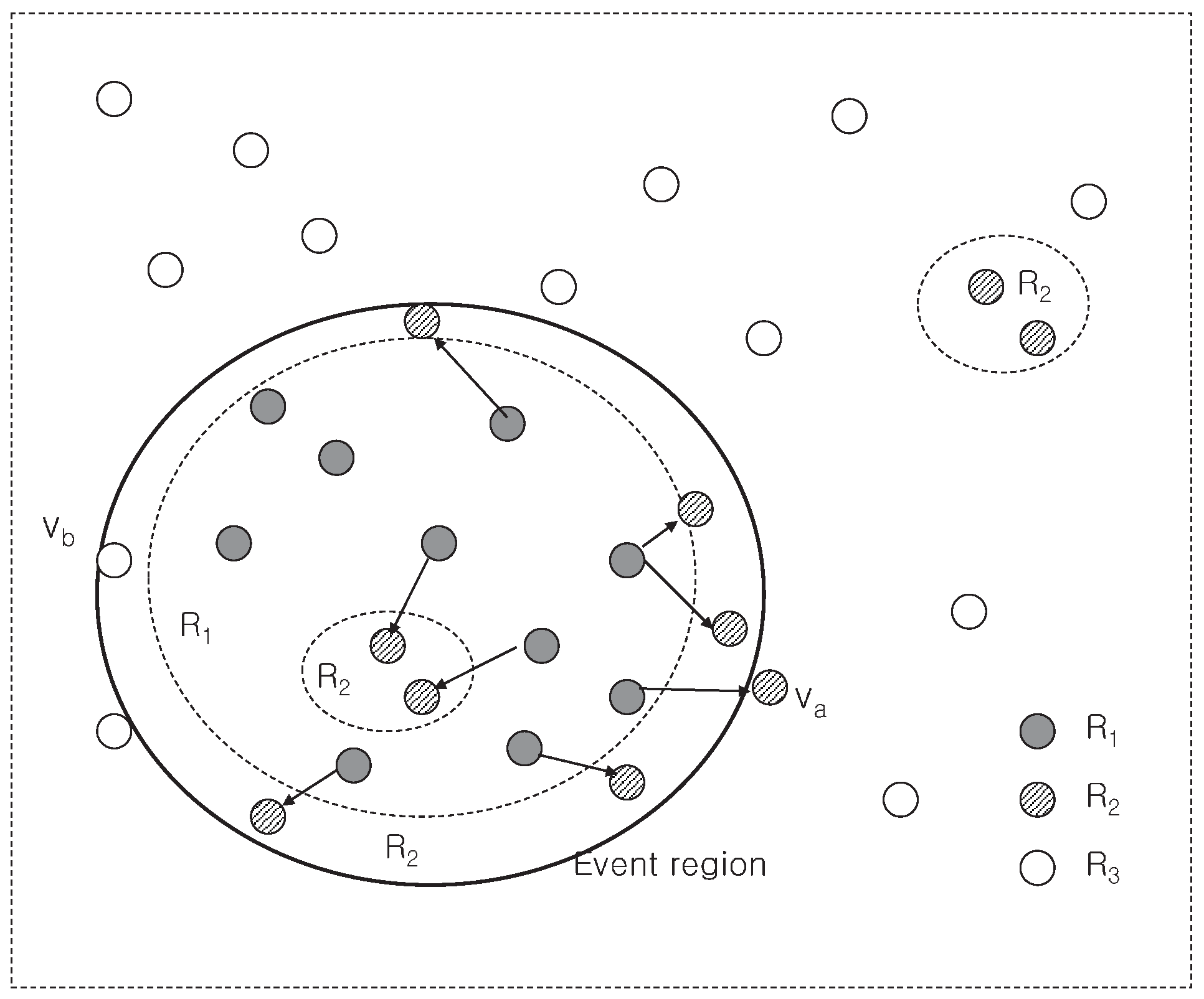
2.1. Network Model and Event Model

In malicious node detection, we assume that n sensor nodes, $\{v_1,v_2,....,v_n\}$, are randomly deployed in the monitored area and have the same transmission range $r_c$. Each sensor node has as its neighbors all the sensor nodes within the transmission range. To represent indirectly the density of a sensor network, we use the average node degree, d, where $d=\frac{{\sum }_{i=1}^n{d}_i}{n}$ and $d_i$ is the degree of node $v_i$.

Events may occur anywhere in the monitored area. The event region is assumed to be a circle with radius $r_e$. When an event occurs, the sensor nodes in the event region report an alarm to their neighbors. Each sensor node then makes a decision on an event based on its own reading and those of its neighbors. Sensed data in this paper are assumed to be binary, 0(normal) or 1(unusual). In the case of an event, normal sensor nodes in an event region are expected to report "1".

2.2. Fault Model

Faults, including malicious nodes, are assumed to occur randomly and independently in any nodes in the network. Three types of faults, transient, permanent and malicious, are considered in this paper. All the sensor nodes are assumed to have a permanent fault with the same probability $p_p$. Both stuck-at-0(normal) and stuck-at-1(unusual) faults are assumed to be equally likely to occur. In addition, normal nodes are assumed to generate incorrect sensor readings due to transient faults with the same probability $p_t$. All the sensor nodes are also assumed to be malicious, with the same probability $p_m$. In the case of malicious nodes, they may report to their neighbors against the actual readings with a probability of $p_{ma}$. If $p_{ma}$ = 0.8, for example, each malicious node reports 1(0) with a probability of 0.8 when the actual reading is 0(1). As $p_{ma}$ approaches 0, it becomes more difficult to identify them due to the similarity in behavior of normal and malicious nodes, and it might also take a longer time to distinguish between them.

3. Malicious Node Detection Using a Dual Threshold

In this section, we present a malicious node detection scheme for wireless sensor networks, where two thresholds, ${\theta }_1$ and ${\theta }_2$, along with trust values, are used to achieve high malicious node detection performance without sacrificing normal nodes.

3.1. Representation of Node Trusts Using a Digraph

Each sensor node $v_i$ maintains a list of its neighbors, $N\left(v_i\right)$, and their trust values from the viewpoint of $v_i$. Trust values are updated each time a local decision on an event is made to reflect the correctness of their reports. Two nodes, $v_i$ and $v_j$, are neighbors of each other if their distance is less than or equal to $r_c$. To represent the trust values we use a weighted directed graph, where the weight $w_{ij}$, ranging between 0 and 1, represents the trust value of node $v_j$ from the viewpoint of $v_i$. If $w_{ij}$ = 1, for example, node $v_i$ totally trusts $v_j$. On the other hand, if $w_{ij}$ = 0, it does not trust $v_j$ at all. In addition, $v_i$ also has its own trust value, $w_{ii}$, ranging from 0 to 1. Once $w_{ii}$ reaches 0, a flag $F_i$ is set to 1, indicating that node $v_i$ is faulty (including malicious). An illustration is given in Figure 1, where node $v_3$ in the center has six neighboring nodes. The number in the node $v_3$ denotes $w_{33}$. The numbers associated with the six edges represent the trust values of the neighboring nodes at $v_3$ (i.e., $w_{3j}$). In the figure, $v_3$ totally trusts $v_2$, while it does not give high trust to the node $v_7$.

Figure 1. A representation of trust values using a digraph.

Figure 1. A representation of trust values using a digraph.

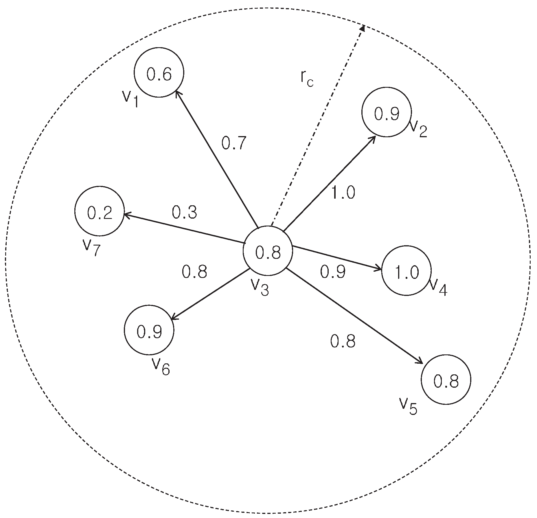
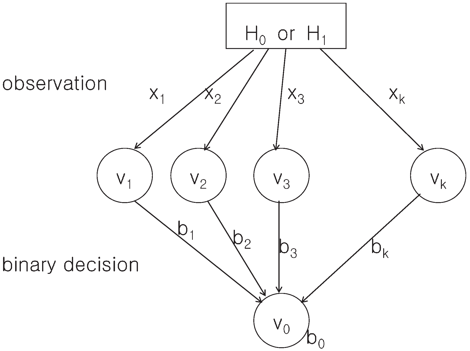
3.2. Modeling Event Detection Problem

The event detection problem is modeled as a hypothesis test problem [9], as shown in Figure 2, where each sensor node determines whether an unknown binary hypothesis is $H_0$ or $H_1$, based on its own reading and those of its neighbors. Each sensor node $v_i$ makes its own binary decision $b_i$ based on the sensor reading $x_i$. These decisions from k neighboring sensor nodes are combined for the final decision. If majority voting is used, for example, $v_0$ in the figure will decide $H_1$ if ${\sum }_{i=0}^k{b}_i>\lceil \frac{k}{2}\rceil$. Our malicious node detection scheme is based on two threshold tests where trust values of the sensor nodes are reflected in the tests.

3.3. Event Detection Using a Dual Threshold

In event detection, each sensor node makes a local decision based on the sensor readings of itself and its neighboring nodes. Two thresholds, ${\theta }_1$ and ${\theta }_2$ (${\theta }_1\ge {\theta }_2$), along with trust values (as weights) of neighboring nodes, are used to make a final decision on an event. The results are used in updating trust values of the associated sensor nodes and identifying malicious nodes.

The threshold, ${\theta }_1$, is used to detect an event while maintaining low false alarm rates. Event nodes on or near the boundary of an event region are likely to fail the test if it has more neighbors outside the event region than inside. The threshold, ${\theta }_2$, helps them pass the test, resulting in more accurate event region detection accuracy.

Figure 2. Distributed event detection.

Figure 2. Distributed event detection.

After receiving the readings of all its neighbors, each sensor node computes the sum of weights of nodes reporting 1, $U_1$ and that of weights of nodes reporting 0, $U_0$. It then applies the high and low thresholds, ${\theta }_1$ and ${\theta }_2$, to $\frac{U_1}{U_0+U_1}$ to determine which group it belongs to. The results divide all the sensor nodes into three groups: $R_1$, $R_2$ and $R_3$, where $R_1$ and $R_2$ are groups of nodes that pass ${\theta }_1$ and ${\theta }_2$ (but fail to pass ${\theta }_1$), respectively. All the remaining nodes are in the group $R_3$. Each sensor node in $R_2$ is reconsidered and indirectly determined to be an event node if it has a neighbor in $R_1$.

An illustration is given in Figure 3, where there is an event region and sensor nodes are divided into three groups ($R_1$, $R_2$, $R_3$) based on the threshold tests. Some event-nodes are in $R_2$. Most of them are on or near the boundary of the event region, although some of them are surrounded by sensor nodes in $R_1$. Non-event-nodes in the right upper corner form a group and pass the test with ${\theta }_2$. They, however, will be determined to be non-event nodes, since they do not have a neighbor in $R_1$. Sensor nodes in $R_2$ inside the event region are likely to be determined to be event nodes with the aid of nodes in $R_1$. Some non-event nodes (e.g., $v_a$) near, but outside, the event region, however, might also be determined to be event nodes if they pass ${\theta }_2$ and have a neighbor in $R_1$. An event-node, such as $v_b$ in Figure 3, on the other hand, can be determined to be a non-event node if it fails both tests.

Figure 3. Dividing sensor nodes into three groups, $R_1$,$R_2$ and $R_3$, using two thresholds.

Figure 3. Dividing sensor nodes into three groups, $R_1$,$R_2$ and $R_3$, using two thresholds.

The role of the threshold ${\theta }_1$ is to minimize the false alarm rate. In most cases, a weighted majority voting (i.e., ${\theta }_1$ = 0.5) will achieve high performance. The threshold, however, needs to be higher, especially when the average node degree is low or fault probabilities are relatively high. An optimal value of ${\theta }_2$ can be determined based on the values of $r_e$ and $r_c$. If $r_e>>r_c$, a sensor node at the event boundary is likely to have the same number of event and non-event nodes within its sensing range. If $r_e$ = $r_c$, on the other hand, only about 39% of the nodes within the sensing range are event nodes. Hence, ${\theta }_2$ = 0.4 will be used in the simulation later.

3.4. Updating Trust Values to Detect Malicious Nodes

Two trust values (weights), $w_{ij}^0$ and $w_{ij}^1$, are used to represent the trustworthiness of node $v_j$ from the viewpoint of $v_i$. Here, $w_{ij}^0$ denotes the trust value of $v_j$ in the case of no-event, while $w_{ij}^1$ denotes the trust value of $v_j$ in the case of an event. Employing two weights eliminates the cancellation effect due to transitions between event and no-event states. In the threshold tests of the previous subsection, $min(w_{ij}^0,w_{ij}^1)$ needs to be used as the weight $w_{ij}$. Depending on the results of the tests, the following updates are performed to reflect the correctness of the current reports in the weights.

In the case of no-event, sensor nodes which are faulty or report a 1 lose their weights as follows:

$$w_{ij}^0=\left\{\begin{array}{cc}\text{max}(0,w_{ij}^0-\alpha )\hfill & \text{for}{b}_j=1\text{or}{F}_j=1\hfill \\ \text{min}(1,w_{ij}^0+\beta )\hfill & \text{for}{b}_j=0\hfill \end{array}\right.$$

(1)

Similarly, the weight of node $v_i$ itself is also updated as follows:

$$w_{ii}^0=\left\{\begin{array}{cc}\text{max}(0,w_{ii}^0-\alpha )\hfill & \text{for}{b}_i=1\hfill \\ \text{min}(1,w_{ii}^0+\beta )\hfill & \text{for}{b}_i=0\hfill \end{array}\right.$$

(2)

The above updates lower the weights of sensor nodes reporting a 1 by α. Sensor nodes with correct readings, on the other hand, recover their weights by β. During this process, nodes with a transient or stuck-at-1 fault and malicious nodes reporting 1 intentionally lose their weights. Nodes with a stuck-at-0 fault gain more weights, although their trust values are bounded above by 1.

In the case of an event, nodes in an event region are expected to report 1. Malicious nodes in an event region reporting 0 intentionally to lead to an incorrect decision, along with the nodes with a stuck-at-0 fault, are now the target of the updates. Since the exact boundary of an event region is not easy to figure out, relatively conservative updates are performed not to sacrifice normal nodes near the event boundary, unless some recovery measures are taken.

For $v_i\in R_1\cup R_2$ and $v_j\in R_1$,

$$w_{ij}^1=\left\{\begin{array}{cc}\text{max}(0,w_{ij}^1-\alpha )\hfill & \text{for}{b}_j=0\text{or}{F}_j=1\hfill \\ \text{min}(1,w_{ij}^1+\beta )\hfill & \text{for}{b}_j=1\hfill \end{array}\right.$$

(3)

Similarly, the weight of node $v_i$ itself is also updated as follows:

For $v_i\in R_1$

$$w_{ii}^1=\left\{\begin{array}{cc}\text{max}(0,w_{ii}^1-\alpha )\hfill & \text{for}{b}_i=0\hfill \\ \text{min}(1,w_{ii}^1+\beta )\hfill & \text{for}{b}_i=1\hfill \end{array}\right.$$

(4)

In updating the weights, two parameters α and β play an important role. It affects the detection rate and detection time of malicious nodes. Some normal nodes can be sacrificed if α becomes larger. For given $p_t$ and $p_{ma}$, the conditional probability that a malicious node reports data opposite to the ground truth, $P_{inv}$, can be written as:

$$P_{inv}=p_t(1-p_{ma})+(1-p_t)p_{ma}$$

(5)

Let $N_d$ denote the average number of no-event cycles required for detecting malicious nodes. Then, for given α and β, the response time, $N_d$, can be derived as follows:

$$N_d(P_{inv}(-\alpha )+(1-P_{inv})\beta )=-1$$

(6)

where no false alarms are assumed to occur for simplicity. At each no-event cycle, a malicious node loses its weight by α with probability $P_{inv}$ or gains its weight by β with probability 1-$P_{inv}$. The node will be determined to be malicious at the time the weight $w_{ij}$, initialized to 1, reaches 0.

Hence, $N_d$ can be given by:

$$N_d=\frac{1}{P_{inv}·\alpha -(1-P_{inv})\beta }$$

(7)

If α = 0.1, β = 0.02, $p_t$ = 0.1, $p_{ma}$ = 0.2, for example, $P_{inv}$ = 0.26 and $N_d$ = $\frac{1}{0.26\times 0.1-0.74\times 0.02}$≈89. That is, malicious nodes are expected to be detected in about 90 cycles on average. As $p_{ma}$ increases, $N_d$ decreases accordingly. Doubling the values of α and β will reduce $N_d$ in half, while normal nodes are more likely to be determined to be faulty. In addition, the ratio $\frac{\alpha }{\beta }$ plays an important role in filtering transient faults and widening the range of $p_{ma}$ to be covered.

Our malicious node detection scheme consists of five steps as follows. Without loss of generality, sensor reading, $x_j$, is assumed to be the binary decision $b_j$ made at the sensor node $v_j$. In Step 1, each sensor node receives the readings of all its neighbors. Each node then computes the sum of the weights of nodes reporting 1, $U_1={\sum }_{j=1}^d{w}_{ij}\times b_j$ and that of the weights of nodes reporting 0, $U_0={\sum }_{j=1}^d{w}_{ij}\times (1-b_j)$, in Step 2. Step 3 applies the two thresholds, ${\theta }_1$ and ${\theta }_2$, to $\frac{U_1}{U_0+U_1}$, to divide the nodes into three groups: $R_1$, $R_2$ and $R_3$, where $R_3$ includes all the nodes that failed both tests. In Step 4, each sensor node in $R_2$ is reconsidered and determined to be an event-node if it has a neighbor in $R_1$. That is, sensor nodes in $R_1$ help sensor nodes in $R_2$ make a final decision indirectly. In Step 5, each sensor node updates the weights of its neighboring nodes according to the given updating policies. It also updates its own weight. Sensor nodes with the trust value of 0 (i.e., a predefined lower bound) are treated as faulty or malicious. They are logically isolated from the rest of the network, unless some recovery actions are taken.

Malicious Node Detection Scheme

1. Obtain the sensor readings $b_j^{\prime }s$ of neighbors of $v_i$

2. Compute $\frac{U_1}{U_0+U_1}$ at each node $v_i$

3. Divide the n nodes into three groups $R_1$,$R_2$ and $R_3$

$v_i\in R_1$ if $\frac{U_1}{U_0+U_1}>{\theta }_1$

$v_i\in R_2$ if ${\theta }_2<\frac{U_1}{U_0+U_1}\le {\theta }_1$

$v_i\in R_3$ otherwise

4. If $|R_1|\ne$0, then H = 1 (i.e., an event)

Determine that $v_i$ is an event node if ($v_i\in R_1$) or ($v_i\in R_2$, $v_j\in R_1$, $v_j\in N\left(v_i\right)$)

If $|R_1|=$0, then H = 0 (i.e., no-event)

5. Update weights, $w_{ii}$ and $w_{ij}$, accordingly

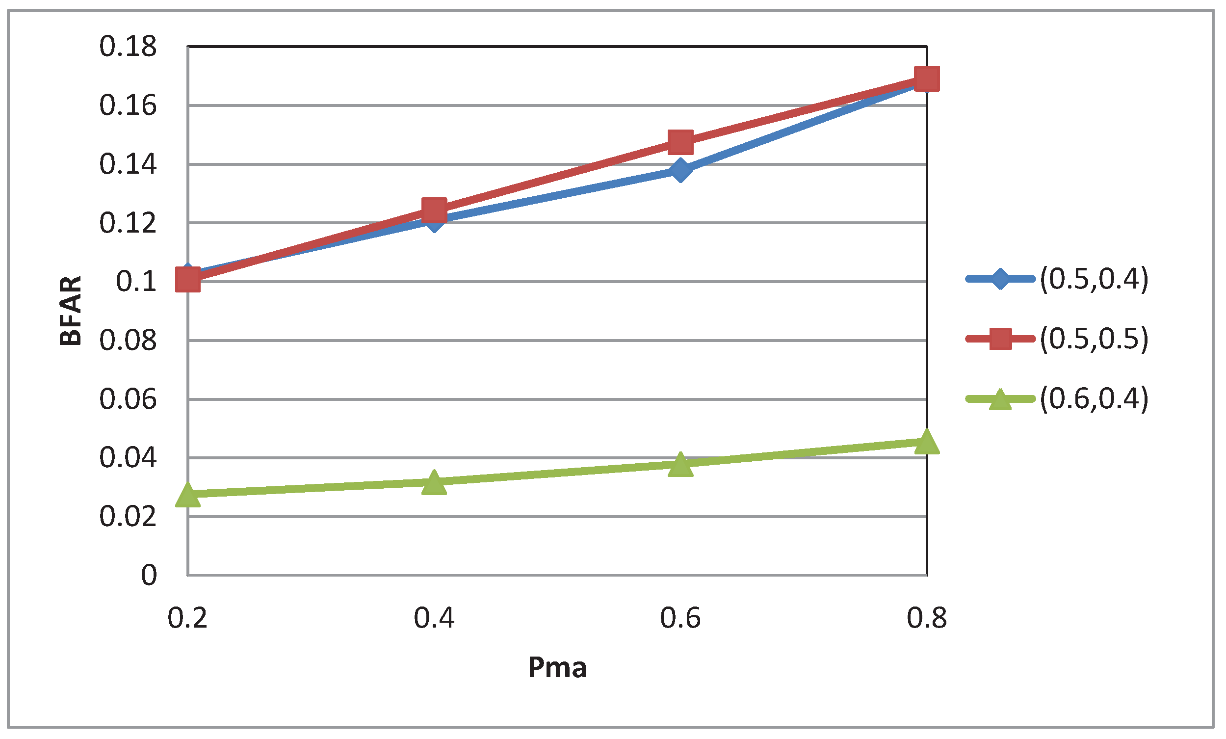
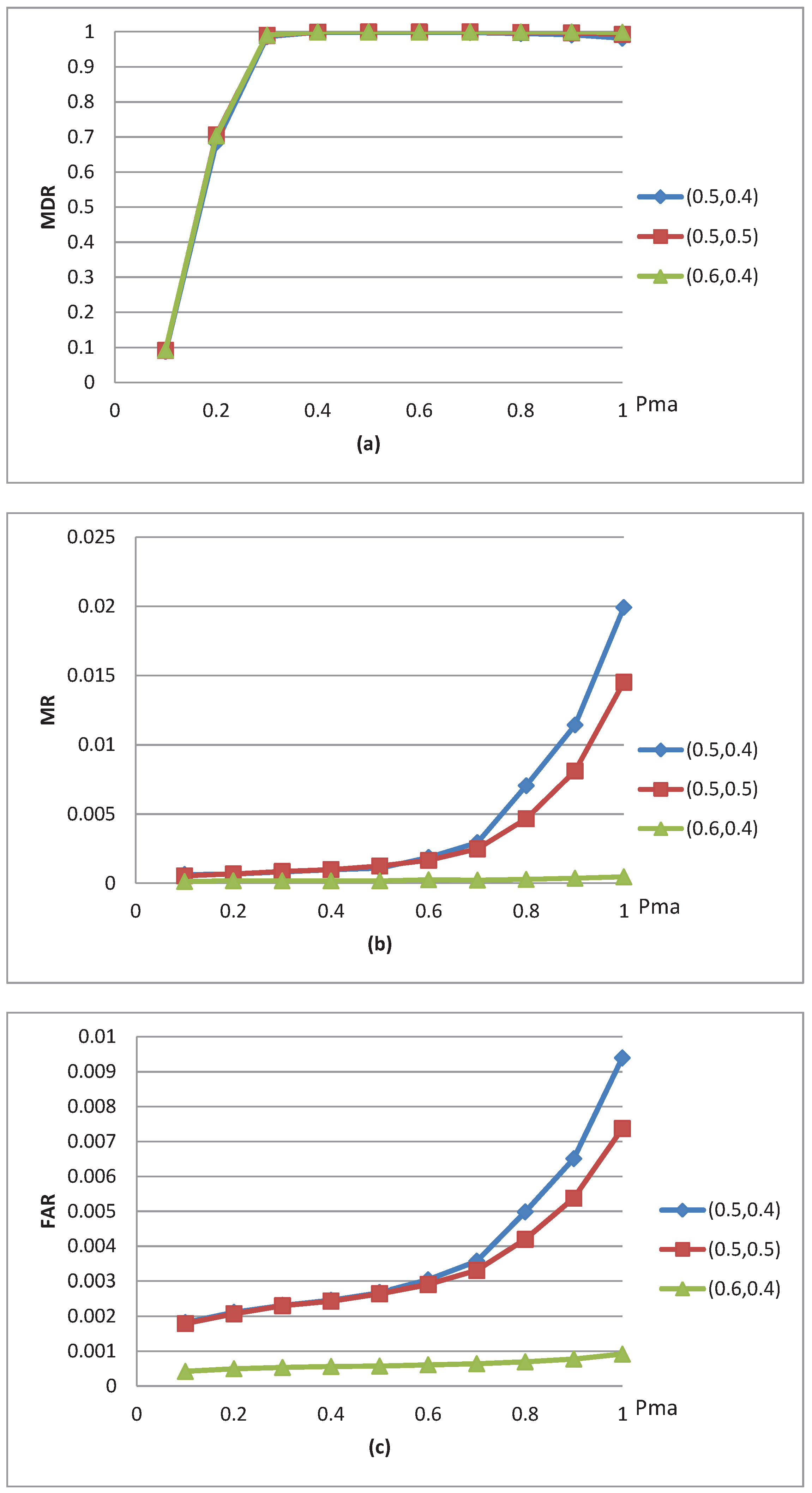
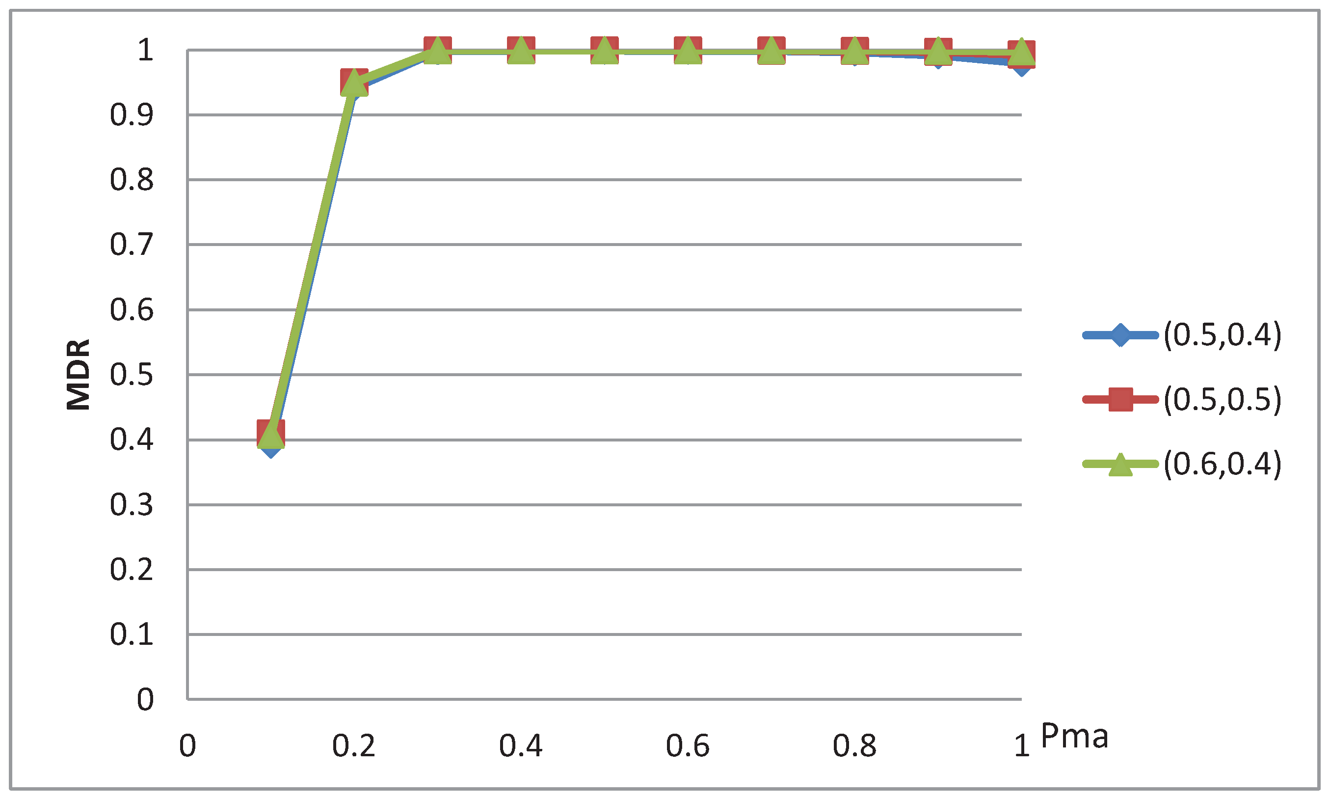
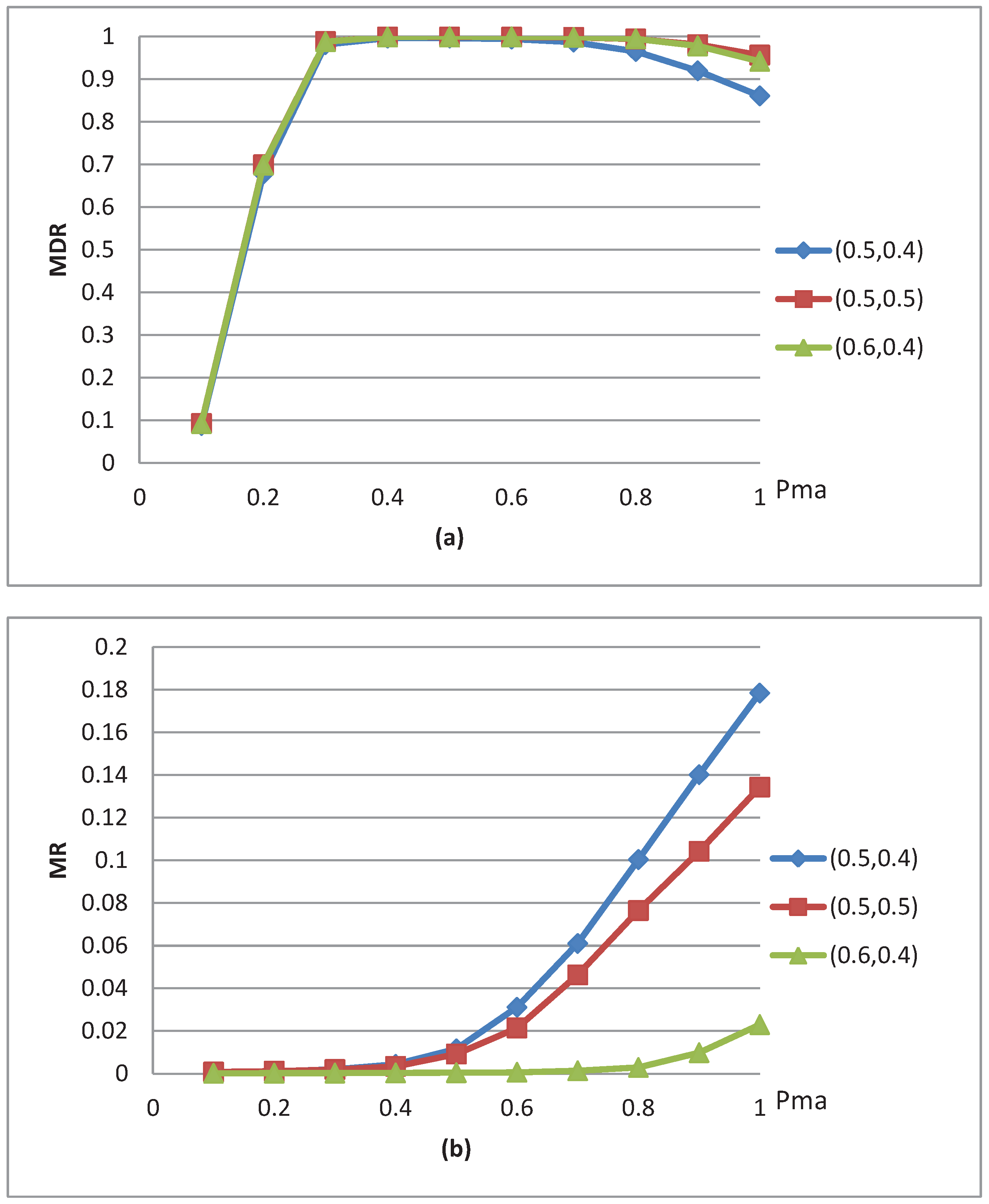
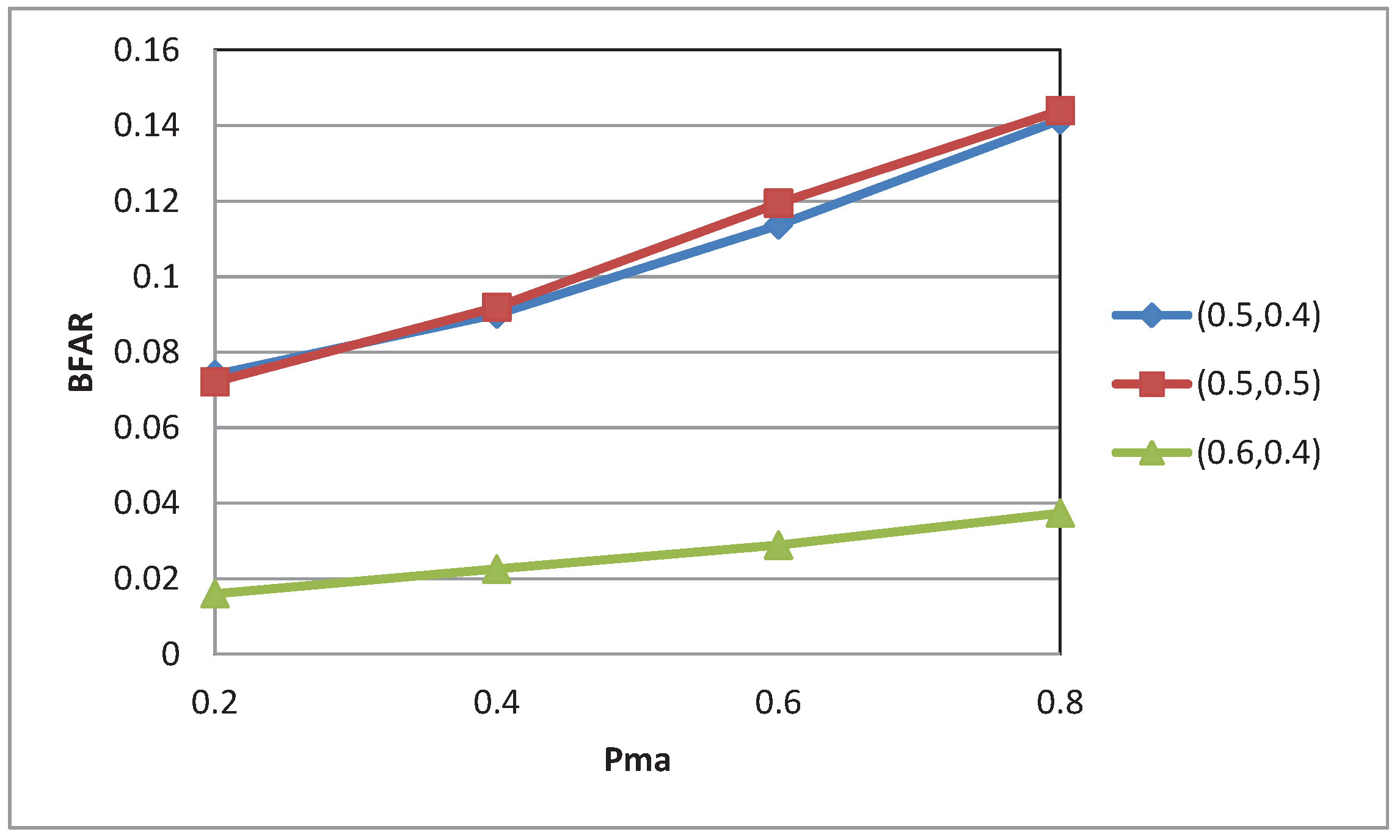
4. Performance Evaluation

4.1. Simulation Setup

Computer simulation is conducted to evaluate the performance of the proposed malicious node detection scheme. It is carried out in a sensor network, where sensor nodes are randomly deployed in a square region. The transmission range $r_c$ is chosen for the sensor network to have the average node degree d = 12. Event regions are assumed to be a circle with radius $r_e$.

Faults and malicious nodes are generated randomly and independently in accordance with predefined probabilities, $p_t$ (transient fault), $p_p$ (permanent fault) and $p_m$ (malicious node). If $p_t$ = 0.1, for example, normal nodes are expected to report incorrect readings with a probability of 0.1. In the case of permanent faults, both stuck-at-0 and stuck-at-1 are assumed to occur with the same probability. If $p_p$ = 0.1, for example, both stuck-at-1 and stuck-at-0 occur with a probability of 0.05 each. In addition, $p_p$ is increased by 0.02 every 20 cycles up to 0.1, to reflect the gradual increase in the number of nodes with a permanent fault. Malicious nodes are generated with probability $p_m$. They are assumed to report opposite to their readings with probability $p_{ma}$.

Six metrics, malicious node detection rate (MDR), misdetection rate (MR), false alarm rate (FAR), event detection accuracy (EDA), event region detection rate (ERDR) and boundary false alarm rate (BFAR), are used to show the effectiveness of our scheme. MDR is defined to be the ratio between the number of detected malicious nodes and the total number of malicious nodes. MR is defined to be the ratio between the number of normal nodes determined to be faulty and the total number of normal nodes. FAR is defined as the ratio of the number of false alarm nodes to the total number of nodes. EDA is the ratio of the number of events correctly detected to the total number of events generated. ERDR, the ratio of the number of event nodes correctly identified to the total number of sensor nodes in the event region, is defined to evaluate the event region detection accuracy. Finally, BFAR is used here to estimate the false alarms very close to the event region. It is defined as the ratio of the number of false alarm nodes one hop away from the event region to the total number of nodes one hop away from the event region.

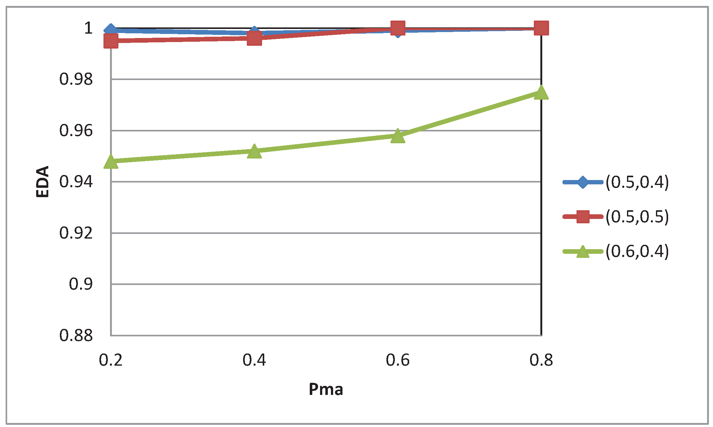
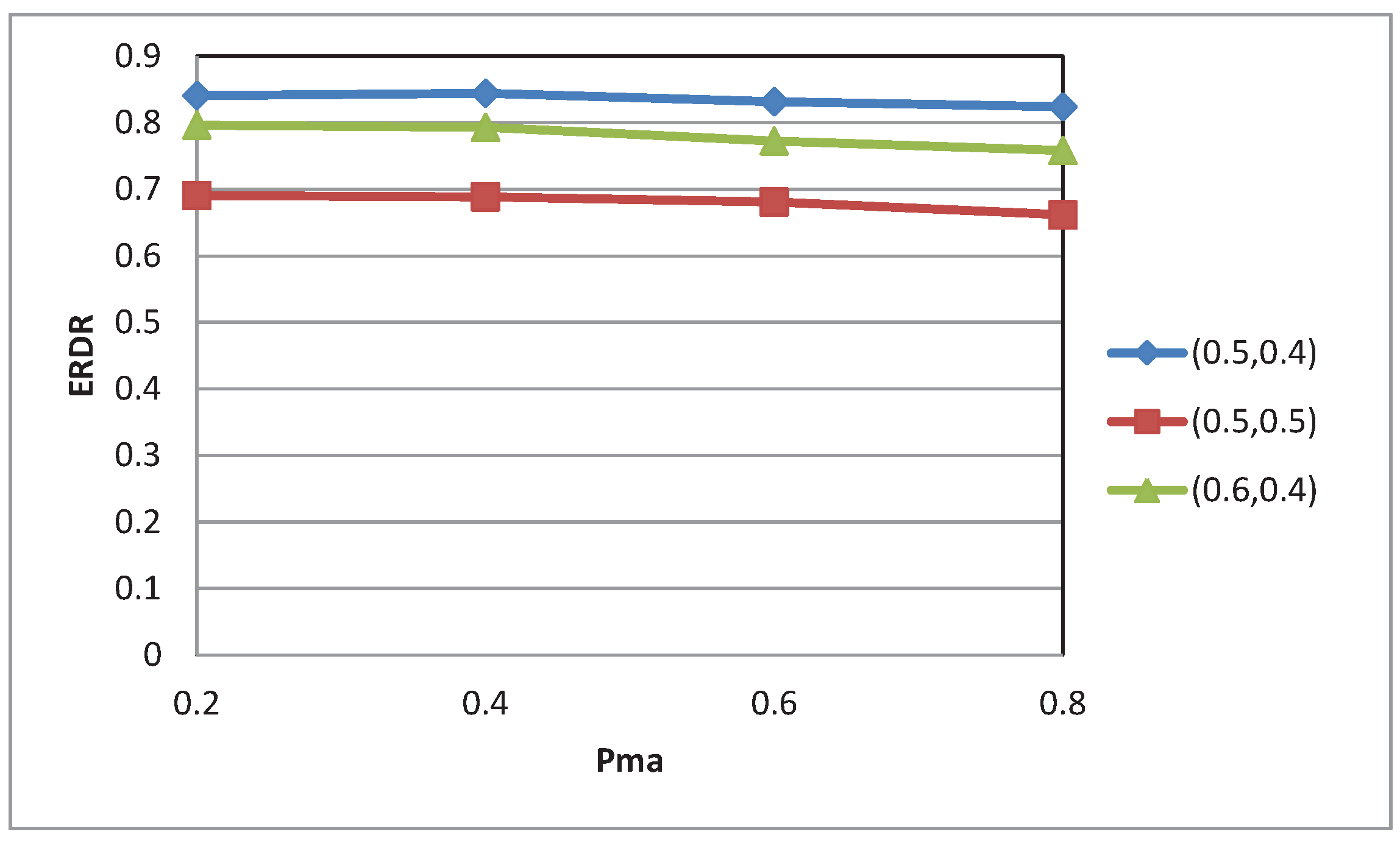
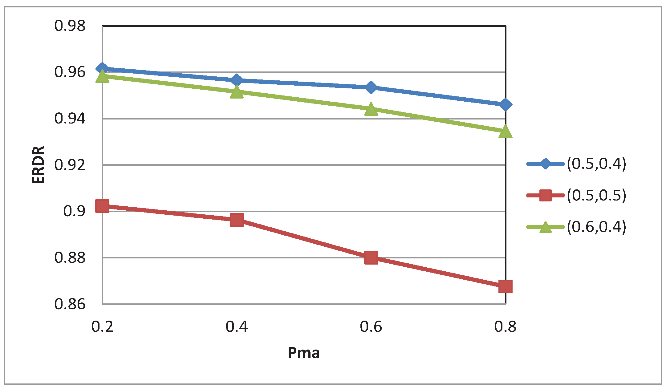
4.2. Experimental Results

Malicious node detection schemes have to achieve high MDR while maintaining low MR. They also need to maintain high EDA while keeping FAR extremely low. In addition, ERDR and BFAR that help identify malicious nodes in an event region also need to be high and low, respectively.

To show the effectiveness of the proposed scheme, we first performed a simulation to estimate MDR, MR and FAR for various values of $p_{ma}$ when d = 12, $p_t$ = 0.1, $p_p$ = 0.1, $p_m$ = 0.1, α = 0.1 and β = 0.02. The results after 100 cycles of operation are shown in Figure 4, where three different values of (${\theta }_1$,${\theta }_2$), (0.5,0.4), (0.5,0.5) and (0.6,0.4) are chosen for comparison purposes.

MDR for $p_{ma}>$0.2 are very close to 1 for all the three cases under comparison, as shown in Figure 4(a) since $\frac{\alpha }{\beta }$ = 5. For the chosen values of α and β, even the nodes reporting a 1 every five cycles on average lose their weights to be eventually detected. As $p_{ma}$ approaches 0, malicious nodes behave similar to normal nodes. Hence, it is not easy to detect them, although they do not cause any significant harm. Further improvements in MDR, as long as $P_{inv}>p_t$, can be made by decreasing the value of β accordingly. MDR for α = 0.1 and β = 0.0125 instead is shown in Figure 5, where notable improvements in MDR are observed for relatively small values of $p_{ma}$. Since $\frac{\alpha }{\beta }\approx$8 in that case, sensor nodes reporting a 1 every eight cycles still lose their weights with time to be eventually detected. If $p_t$ = 0.1 and $p_{ma}$ = 0.1, for example, $P_{inv}$ = 0.1 × 0.9 + 0.9 × 0.1 = 0.18. Hence, malicious nodes with $p_{ma}$ = 0.1, when $p_t$ = 0.1, report a 1 every five cycles, approximately, and thus, they cannot remain undetected, although it takes more time to detect them.

As far as MR is concerned, a dual threshold of 0.6 and 0.4 outperforms the other two and shows persistent performance regardless of the value of $p_{ma}$, as shown in Figure 4(b).

FAR should be kept low, since frequent alarms due to incorrect decisions shorten the network lifetime and might break the network function. FAR for a dual threshold of (0.6,0.4) is much better than that for a single threshold of 0.5, as shown in Figure 4(c). FAR for the single threshold and the dual threshold of (0.5,0.4) increases with $p_{ma}$, while FAR for (0.6,0.4) is kept extremely low for the entire range of $p_{ma}$.

We then performed the same simulation after changing $p_m$ to 0.2. Similar trends are observed for the single and dual thresholds, as shown in Figure 6. When $p_{ma}$ is close to 1, however, MDR drops slightly. This is due to the fact that all the malicious nodes in the extreme case act like a faulty node with a permanent fault. Hence, doubling $p_m$ causes more false alarms as $p_{ma}$ approaches 1. Consequently, the trust values of some malicious nodes cannot be lowered, resulting in a small decrease in MDR.

MR for $p_m$ = 0.2, shown in Figure 6(b), is much higher than that for $p_m$ = 0.1, although the trend is very similar. The scheme with a dual threshold of (0.6,0.4), although the small increase in MR is unavoidable, still maintains a relatively consistent performance.

Figure 4. Malicious node detection rate (MDR), misdetection rate (MR) and false alarm rate (FAR) for various values of $p_{ma}$ when α = 0.1 and β = 0.02.

Figure 4. Malicious node detection rate (MDR), misdetection rate (MR) and false alarm rate (FAR) for various values of $p_{ma}$ when α = 0.1 and β = 0.02.

The proposed scheme is designed for malicious node detection. However, the resulting event detection performance also needs to be maintained high. EDA strongly depends on the value of ${\theta }_1$, since at least one node in an event region must pass the threshold to detect an event. As shown in Figure 7, EDA for the single threshold of 0.5 and EDA for the dual threshold of (0.5,0.4) are better than that for the dual threshold of (0.6,0.4) when $p_t$ = 0.1, $p_m$ = 0.2 and $r_e$ = $r_c$. As $r_e$ increases, however, it is almost guaranteed that at least one node can pass the test with ${\theta }_1$. The resulting EDAs for $r_e$ = $2r_c$ are almost perfect for all three cases under comparison.

Figure 5. MDR for various values of $p_{ma}$ when α = 0.1 and β = 0.0125.

Figure 5. MDR for various values of $p_{ma}$ when α = 0.1 and β = 0.0125.

Figure 6. MDR and MR for various values of $p_{ma}$ when $p_t$ = 0.1, $p_m$ = 0.2 and $p_p$ = 0.1.

Figure 6. MDR and MR for various values of $p_{ma}$ when $p_t$ = 0.1, $p_m$ = 0.2 and $p_p$ = 0.1.

Figure 7. EDA for $r_e=r_c$, α = 0.1 and β = 0.02.

Figure 7. EDA for $r_e=r_c$, α = 0.1 and β = 0.02.

Event region detection accuracy plays an important role in malicious node detection, since malicious nodes reporting 0 in an event region can be identified during the event period. To estimate the effectiveness of the scheme in detecting event regions, the simulation is extended to obtain ERDR and BFAR for various values of $p_{ma}$, when $p_t$ = 0.1, $p_{ma}$ = 0.2 and $r_e$ = $r_c$. The results are shown in Figure 8 and Figure 9, respectively.

Figure 8. event region detection rate (ERDR) for various values of $p_{ma}$, when $r_e=r_c$.

Figure 8. event region detection rate (ERDR) for various values of $p_{ma}$, when $r_e=r_c$.

Figure 9. and boundary false alarm rate (BFAR) for various values of $p_{ma}$ when $r_e=r_c$.

Figure 9. and boundary false alarm rate (BFAR) for various values of $p_{ma}$ when $r_e=r_c$.

The scheme with a dual threshold of (0.5,0.4) performs the best among the three cases under comparison as far as ERDR is concerned. ERDR for the scheme with a single threshold of 0.5 is significantly lower than the other two, as shown in Figure 8. As far as BFAR is concerned, a dual threshold of (0.6,0.4) outperforms the other two, as shown in Figure 9. Significantly higher ERDR is observed when $r_e$ = $2r_c$ for all three cases under comparison, as shown in Figure 10. A slight increase in BFAR is also observed for each of the three cases, as shown in Figure 11, although the trends are similar. Consequently, we suggest to use two thresholds of 0.6 and 0.4 in event region detection to correctly identify malicious nodes behaving against the ground truth. Finally, the thresholds can be dynamically adjusted depending on the applications to optimize the malicious node detection performance.

In the development of the proposed detection scheme, all the nodes are treated equally. It might be worth considering for a sensor node to place more weight on its own reading than those of its neighbors, as far as event boundary detection is concerned. For a malicious node in the corner of the network area or with very few neighbors, it might be easy to pass the threshold if the neighbors are faulty or malicious almost at the same time. Even when the node claims itself to be normal, it is highly likely to be isolated from the rest of the network, due to the surrounding normal nodes.

Figure 10. ERDR for various values of $p_{ma}$, when $r_e=2r_c$.

Figure 10. ERDR for various values of $p_{ma}$, when $r_e=2r_c$.

Figure 11. BFAR for various values of $p_{ma}$, when $r_e=2r_c$.

Figure 11. BFAR for various values of $p_{ma}$, when $r_e=2r_c$.

5. Conclusions

In this paper, a malicious node detection scheme using a dual threshold in wireless sensor networks is presented. Each sensor node maintains trust values of neighboring nodes to reflect their past behavior in decision-making. Two thresholds are used to reduce the false alarm rate and enhance the event region detection accuracy, resulting in more accurate malicious node detection performance without sacrificing normal nodes. Simulation results have shown that the scheme with a dual threshold outperforms that with a single threshold. The proposed scheme employs a few parameters whose values can be properly chosen depending on applications. They can also be dynamically adjusted, if necessary, to optimize the performance.

References

1. Akyildiz, I.F.; Su, W.; Sankarasubramaniam, Y.; Cyirci, E. Wireless sensor networks: A survey. Comput. Netw. 2002, 38, 393–422. [Google Scholar] [CrossRef]
2. Mainwaring, A.; Polaste, J.; Szewczyk, R.; Culler, D.; Anderson, J. Wireless Sensor Networks for Habitat Monitoring. In Proceedings of the ACM International Workshop on Wireless Sensor Networks and Applications, Atlanta, GA, USA, 28 September 2002; pp. 88–97.
3. Yu, M.; Mokhtar, H.; Merabti, M. Fault management in wireless sensor networks. IEEE Wirel. Commun. 2007, 14, 13–19. [Google Scholar] [CrossRef]
4. Xu, X.; Zhou, B.; Wan, J. Tree Topology Based Fault Diagnosis in Wireless Sensor Networks. In Proceedings of the International Conference on Wirleess Networks and Infomation Systems, Shanghai, China, 28–29 December 2009; pp. 65–69.
5. Lee, M.H.; Choi, Y.-H. Fault detection of wireless sensor networks. Comput. Commun. 2008, 31, 3469–3475. [Google Scholar] [CrossRef]
6. Rajasegarar, S.; Leckie, C.; Palaniswami, M. Anomaly detection in wireless sensor networks. IEEE Wire. Commun. 2008, 15, 34–40. [Google Scholar] [CrossRef]
7. Krishnamachari, B.; Iyengar, S. Distributed Bayesian algorithms for fault-tolerant event region detection in wireless sensor networks. IEEE Trans. Comput. 2004, 53, 241–250. [Google Scholar] [CrossRef]
8. Ding, M.; Chen, D.; Xing, K.; Cheng, X. Localized Fault-tolerant Event Boundary Detection in Sensor Networks. In Proceedings of the IEEE International Conference on Computer Communications, Miami, FL, USA, 13–17 March 2005; pp. 902–913.
9. Luo, X.; Dong, M.; Huang, Y. On distributed fault-tolerant detection in wireless sensor networks. IEEE Trans. Comput. 2006, 55, 58–70. [Google Scholar] [CrossRef]
10. Li, C.-R.; Liang, C.-K. A fault-tolerant event boundary detection algorithm in sensor networks. LNCS 2008, 5200, 406–414. [Google Scholar]
11. Xiang, Y.; Li, H.; Xie, Z.; Li, P. Distributed Weighting Fault-Tolerant Algorithm for Event Region Detection in Wireless Sensor Networks. In Proceedings of the International Conference on Communications, Circuits and Systems, Changsha, China, 25–27 May 2008; pp. 414–418.
12. Cui, X.; Li, Q.; Zhao, B. Data discrimination in fault-prone sensor networks. Wirel. Sens. Netw. 2010, 12, 285–292. [Google Scholar] [CrossRef]
13. Curiac, D.I.; Banias, O.; Dragan, F.; Volosencu, C.; Dranga, O. Malicious Node Detection in Wireless Sensor Networks Using an Autoregression Technique. In Proceedings of the 3rd International Conference on Networking and Services, Athens, Greece, 19–25 June 2007; p. 83.
14. Pires, W.R., Jr.; Figueiredo, T.; Wong, H.; Loureiro, A. Malicious Node Detection in Wireless Sensor Networks. In Proceedings of the 18th International Parallel and Distributed Processing Symposiuim, Santa Fe, NM, USA, 26–30 April 2004.
15. Xiao, X.-Y.; Peng, W.-C.; Hung, C.-C.; Lee, W.-C. Using Sensor Ranks for In-network Detection of Faulty Readings in Wireless Sensor Networks. In Proceedings of the International Workshop Data Engieering for Wireless and Mobile Access, Beijing, China, 10 June 2007; pp. 1–8.
16. Atakli, I.M.; Hu, H.; Chen, Y.; Ku, W.-S.; Su, Z. Malicious Node Detection in Wireless Sensor Networks Using Weighted Trust Evaluation. In Proceedings of the 2008 Spring Simulation Multiconference, Ottawa, Canada, 14-17 April 2008; pp. 836–842.
17. Hu, H.; Chen, Y.; Ku, W.-S.; Su, Z.; Chen, C.-H. Weighted trust evaluation-based malicious node detection for wireless sensor networks. Int. J. Inf. Comput. Security 2009, 3, 132–149. [Google Scholar] [CrossRef]
18. Ju, L.; Li, H.; Liu, Y.; Xue, W.; Li, K.; Chi, Z. An Improved Detection Scheme Based on Weighted Trust Evaluation for Wireless Sensor Networks. In Proceedings of the 5th International Conference on Ubiquitous Information Technologies and Applications, Hainan, China, 16–18 December 2010; pp. 1–6.
19. Momani, M.; Challa, S. Survey of trust models in different network domain. Int. J. Ad hoc Sens. Ubiquitous Comput. (IJASUC) 2010, 1, 1–19. [Google Scholar] [CrossRef]
20. Momani, M.; Challa, S.; Alhmouz, R. Can We Trust Trusted Nodes in Wireless Sensor Networks? In Proceedings of the International Conference Computer and Communication Engineering, Kuala Lumpur, Malaysia, 13–15 May 2008; pp. 1227–1232.