1. Introduction
Many contemporary sensing applications entail the remote, continuous, unattended and
in-situ monitoring of natural processes. Such applications are possible, due to recent developments in the fields of Micro-Electro-Mechanical Systems and Wireless Sensor Networks and can pose technologically challenging demands, which were not
a priori incorporated in the design/optimization criteria for either of these two fields [
1,
2,
3].
For environmental deployment, the production of flexible, robust sensor housings is an essential pre-requisite. Casings affect the overall usefulness of any monitoring system, since they define the limits of
in-situ monitoring without the risk of damage, as well as other practical aspects, such as the ease of recovery or repair. These aspects become even more important in harsh and very variable natural environments, such as the ocean [
4], volcanoes [
5], glaciers [
6] and rivers (on Earth and other planets [
7]), where complex processes take place, the understanding of which is based on the quality of the sensed data.
In parallel with practical considerations, it is crucial to understand how the sensor itself affects the process of data-acquisition, hence the quality of the derived data and the general theoretical context in which such data are analysed. The effects of the physical properties (e.g., shape, weight, density) of the sensor are especially important in the case of inertial sensors that are deployed for monitoring movement (such as accelerometers and gyroscopes), because the sensors inevitably become part of the process.
We are particularly interested in sensors that measure aspects of grain movement in rivers. The work reported here is based upon our experience in constructing wireless sensor systems to perform such measurements. Later phases of the work will address sensor design, power and radio communication aspects. Here, we particularly focus on a repeatable process for generating robust sensor casings that guarantee the physical and electrical integrity of the sensor and enable highly accurate calibration of the sensor in-situ.
1.1. Problem Statement: Motivation
Earth-surface processes often involve the movement of material at scales ranging from single grains to mass movements affecting entire hillslopes [
8]. To assess material transport rates, morphological changes and environmental hazards, a common monitoring strategy is to tag and track a number of individual grains. This approach generates understanding of the displacement of sediment during events, but is often restricted to before- and after-event comparisons. Many methods have been devised to tag tracer grains, ranging from simple visual identification (painting) to very complex and technologically challenging techniques, such as the deployment of magnetic and radio frequency tags [
9,
10,
11].
Advances in sediment transport theory have been delayed by the absence of suitable technology to test theoretical predictions [
12]. The lack of continuous data with accurate positional and timing references precludes reliable mathematical and statistical descriptions of the system, so restricting the use of these predictions [
13].
1.2. Casing Design Criteria Related to the Natural System
The shape of natural sediment grains exerts a strong influence over their movement [
14,
15,
16,
17]. Theoretical analyses, however, have assumed idealised spherical grains (e.g., Wiberg and Smith [
18],
etc.); this simplification makes the solution of the force-balance equations feasible, and the consequent results have been found to have widespread applicability (e.g., Hodge
et al. [
19]). We begin with a spherical case, the performance of which can be precisely evaluated against theory and then generalise to the full range of natural shapes.
As well as grain shape, the density of the sensor must replicate that of natural material. The deployment of sensors, such as accelerometers, is useful only if the sensor behaves as a rigid body of uniform density (something that can be assumed for individual natural grains). The overall density and distribution of mass within the sensor must match those of natural materials without affecting the operation of the device.
The material properties of the case (such as the roughness of the surface or the plasticity) also affect the quality of the data. Experience from previous field studies shows that the design criteria include several environmental factors, such as chemical weathering of the case or its trapping by trees or debris, that affect greatly the long-term deployment of the sensor. These factors cannot be addressed if the system optimization is based exclusively on electronics-computing-related optimization criteria.
1.3. Scope and Structure of the Paper
Here, we present the first results from the development of a new mobile sensor, designed for acquiring data representative of the instantaneous forces experienced by individual pebbles in a river or a similar natural environment. We present a general framework that can potentially address one of the key challenges, the construction of adequate sensor casings. We discuss how the combination of available 3D modelling tools and fast prototyping technology (3D printing) speeds up the development process and has the potential to enhance the coherence of the sensed data.
Section 2 provides an overview of previous work, addressing the core limitations that restrict the deployment of this type of sensor and reviews common approaches to sensor housing in underwater environments. In
Section 3, we describe the prototyping method and how it enhances the securing of the sensor and the representativeness of the derived data. In
Section 4, we describe initial test results from a prototype sensor and housing and assess these results in the context of potential field deployment of the system. In
Section 5, we summarize the key points.
2. Previous Relevant Work
2.1. Sediment Transport Sensing
A number of projects have developed ’smart’ loggers, instrumented with suitable sensors that are able to store data, which, in principle, can be used to resolve the actual paths taken by individual grains through post-event analysis [
20,
21,
22]. This approach initially faced many technical challenges in acquiring, storing and transmitting the data [
20,
21]. Recent advances in the field of Micro-Electro-Mechanical Systems have enhanced data acquisition and storage [
23,
24]. However, none of these projects has reached the stage of large-scale field deployment nor has published data that can be interpreted in a theoretical framework of natural sediment movement. The basic limitations are:
Mismatch between the measurement range of the deployed sensors and the magnitude of the physical processes. Instantaneous point forces in natural systems are of greater magnitude than the measurement range of the sensors, and time-averaging leads to underestimates of peak forces. For example, static sensors used to measure river sediment movement record either the number of impacts or the maximum acceleration produced by impacting particles during a predetermined sampling interval [
25,
26]. These measurements are known to underestimate the impact forces on individual grains; however, they do suggest a range of forces the sensor has to operate reliably. Instantaneous vibrations of an order of 100 g [
26] have been recorded, an order of magnitude higher than the measurement range of the inertial accelerometers deployed in the majority of previous applications. An exception was the Smart-Cobble [
21], where the accelerometer alone was capable of capturing peak accelerations of 5,000 g, and the whole sensor had a measuring range of +/−480 g for an non-amplified signal (reducing to an operational range of +/−48 g after analogue amplification). This initial deployment of heavy-duty, high-range accelerometers was not continued in subsequent studies [
23,
24].
The development of robust and representative sensor casings/enclosures. Deployment in natural environments requires durable, long-lasting and waterproof sensor housings. The sensor and housing together require physical characteristics (size, shape, weight, density, roughness) that ensure the representativeness of the data.
The lack of real-time reference. A key limitation is that post-event analysis can be done robustly only in very controlled and well-defined time-space domains (which can be reproduced only in a laboratory setting), making difficult the connection with the real, highly variable conditions in a river system. Aberyawardana
et al. [
23] were able to extract very precise information about the entrainment conditions of a sensor, after a very detailed sensor-calibration process, but the post-event analysis of the data does not permit the accurate resolution of the path followed by their "smart" pebble.
As a result of these issues, sediment movement is currently monitored using techniques that provide information on sediment movement over long time periods. The most advanced techniques involve attaching magnetic or Radio Frequency Identification-tags to natural or artificial pebbles, to identify the initial position of the tracers before a flood, and, then, either try to identify the rest of the positions of the tracers after the flood using hand-held detectors [
27] or combine this technique with the tracking of the position of the tracers as they pass a known downstream position during the transport event, when the process is underway at the time of detection (e.g., [
28,
29]).
2.2. Underwater Sensor Housings
The majority of the existing underwater-sensing equipment concerns oceanographic applications[
30], where there is a general requirement for robustness and long-lasting water-proof performance under very high pressures and harsh conditions. Environmental applications deployed static sensing units until very recently [
1], and underwater sensor mobility is investigated either in the context of robotics and vehicle navigation [
31] or for depth adjustments towards the optimization of underwater acoustic networking techniques [
32]. In rivers, the common sensing equipment used is also static (pressure sensors, chemical sensors,
etc.), and except for not requiring durability under high pressures, the casing requirements are similar to oceanographic applications [
33]. Consequently, the common sensor housing practice is the mounting of the sensors on a steady frame, which is protected by a durable cover made of PVC or metal.
Although the enclosures have never been addressed as a separate research challenge for underwater sensing systems [
34], research has been performed for increasing the lifetime of the case against specific erosion processes, such as bio-fouling [
35]. However, the contemporary casing design criteria do not restrict or specifically define properties, such as the size, the shape or the density of the enclosures, as long as durability is secured.
3. Experimental Section
3.1. Case Design Procedure
Initially, it is critical to ensure that the sensor will not be excessively stressed and will remain dry during operation. The second critical requirement is to keep the sensor immobile and permanently oriented in relation to the final frame of the case. Achieving this integrity would be difficult if the whole design matched a natural shape. Hence, we use a two-part design: (1) an internal case for the sensor that has an internal structure to fit the sensor, holding it in place and keeping it operational; and (2) an outer case that fits rigidly around the first and that defines the overall shape of the sensor.
3.2. Design and Construction of the Internal Case
This phase begins with a 3D representation (a 3D model) of the actual sensor platform around which the inner casing is to be constructed.
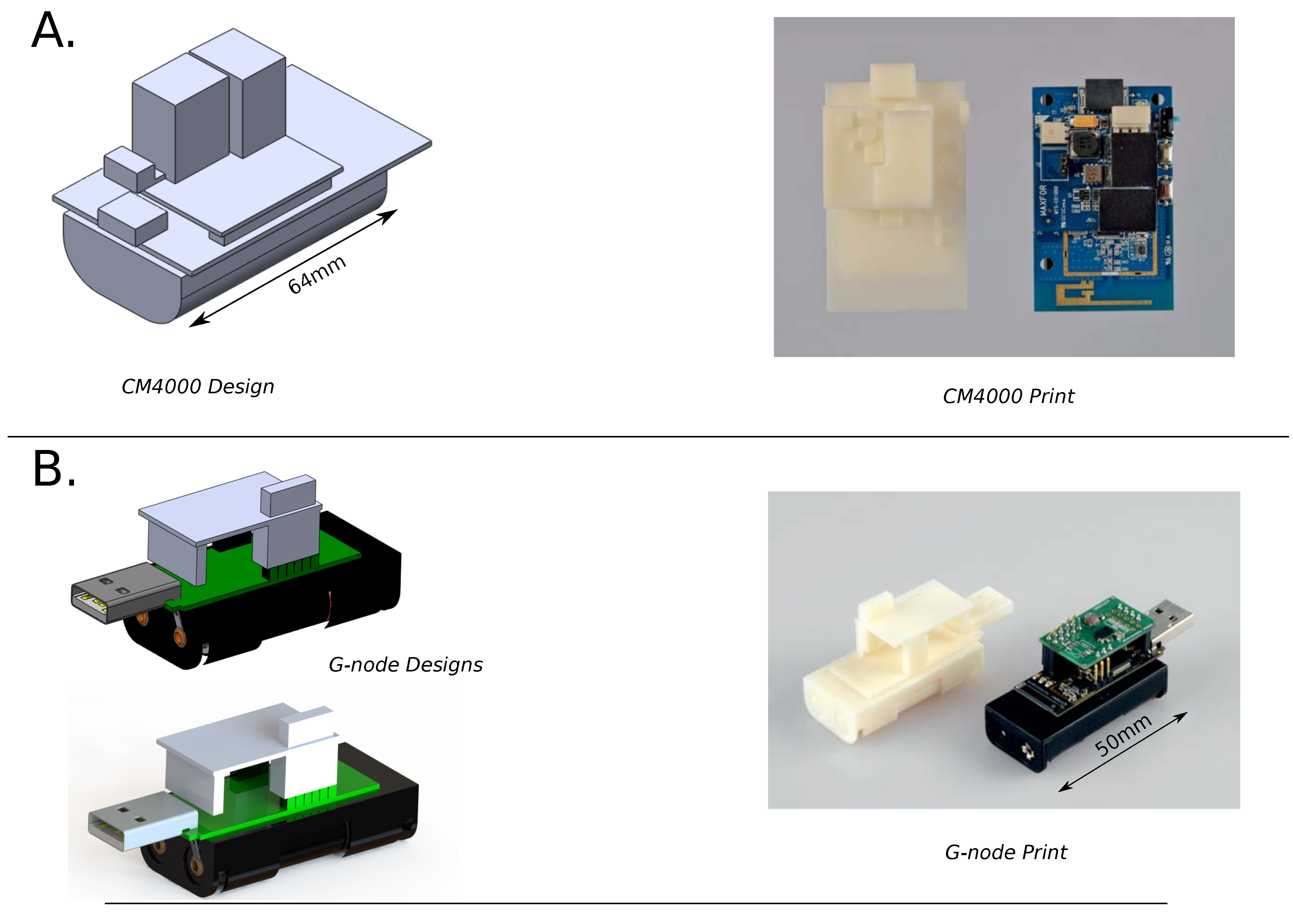
Figure 1 shows the 3D models of two commercial platforms that were tested for this application: the AdvanticSys CM4000 mote platform [
36], with the C01000 sensor platform [
37] attached, and the G-node mote platform with the G-Colta sensor board attached, both produced by SOWNET Technologies [
38] . The G-Colta sensor board is equipped with the ADXL-345 3-axial accelerometer with a maximum measurement range of +/−16 g produced by Analog Devices [
39].
The software used to produce the designs was Solid-Works
TM provided by Dassault Systèmes [
40]. Although the sensor platforms can have relatively complicated 3D structures, it is possible to input the geometrical metrics at a 1:1 scale without significant error. However, a 3D scanner can be used in order to input an initial point-cloud sketch, which can then be manipulated through the software and corrected using manual measurements. The design can then be input into a 3D printer, producing a plastic 3D copy of the sensor’s structure (this step is not essential and is used here for demonstration purposes).
Figure 1 shows the digital and the actual copies for the two sensor platforms.
Figure 1.
3D models of tested sensors: (A) Digital design (left) and 3D printing, right of the CM4000 sensor mote with the compatible attached sensor board (right). The 3D design of the sensor is the base for the design of the case, making the fit exact; (B) Design and 3D printing of the G-node with the compatible G-Colta sensor board.
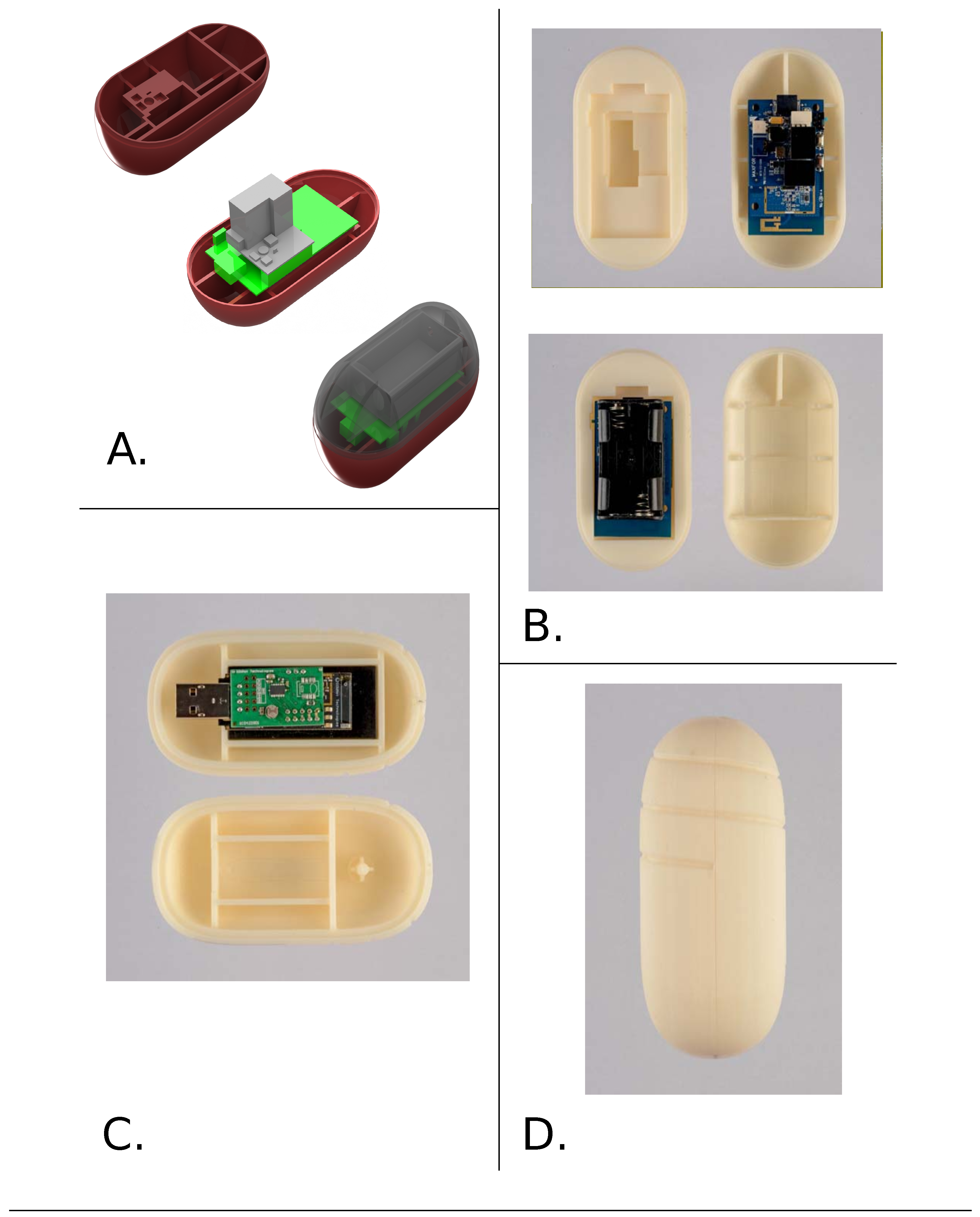
Given the 3D model of the sensor platform as a base, it is possible to modify regular 3D shapes to incorporate the structure of the mote with great accuracy. The tools provided by the software enable the production of regular shapes (like ellipses and cubes), so they have an inertial form shaped as the exact negative of the sensor platform’s 3D structure, while keeping the overall shape unaffected. This exact fit of a void within the regular shape to the sensor platform guarantees that the sensor platform will be immobile within the inner casing and consistently oriented relative to the outer casing. This enables the platform to be calibrated appropriately. Examples of the designs and the constructed internal enclosures are shown in
Figure 2 for the two sensor platforms.
3.3. Outer Case
The initial stage in the process of development of this type of purpose-specific sensor is the testing of commercial, off-the-shelf platforms to assess the level of customization needed to fulfil the requirements of the application. The casing developed for this calibration/evaluation procedure must be idealized and regular in order to permit comparisons. As a result, the methodology was initially developed for idealized enclosures of regular shape and subsequently extended for the construction of cases with more realistic and natural shapes.
Figure 2.
The development of internal case: (A) The sensor is accommodated rigidly by the internal structure of the case, matching the structure of the sensor, shown here for the CM4000 sensor-mote; (B,C) The final 3D printed case fits the sensor accurately, keeping the overall assembly compact and minimizing the movement of the sensor (examples for CM4000 (B) and G-node (C)); (D) Modifications can be made to accommodate special features, such as the modified antenna of the G-node, which can be secured within the spiral sculptured into the external surface of the case constructed for the G-node (D).
3.3.1. Cases of Regular Shape
We use the inner case as a base around which to construct an outer case that has a desirable shape. As previously, the software tools enable the enclosure of the inner case with high precision.
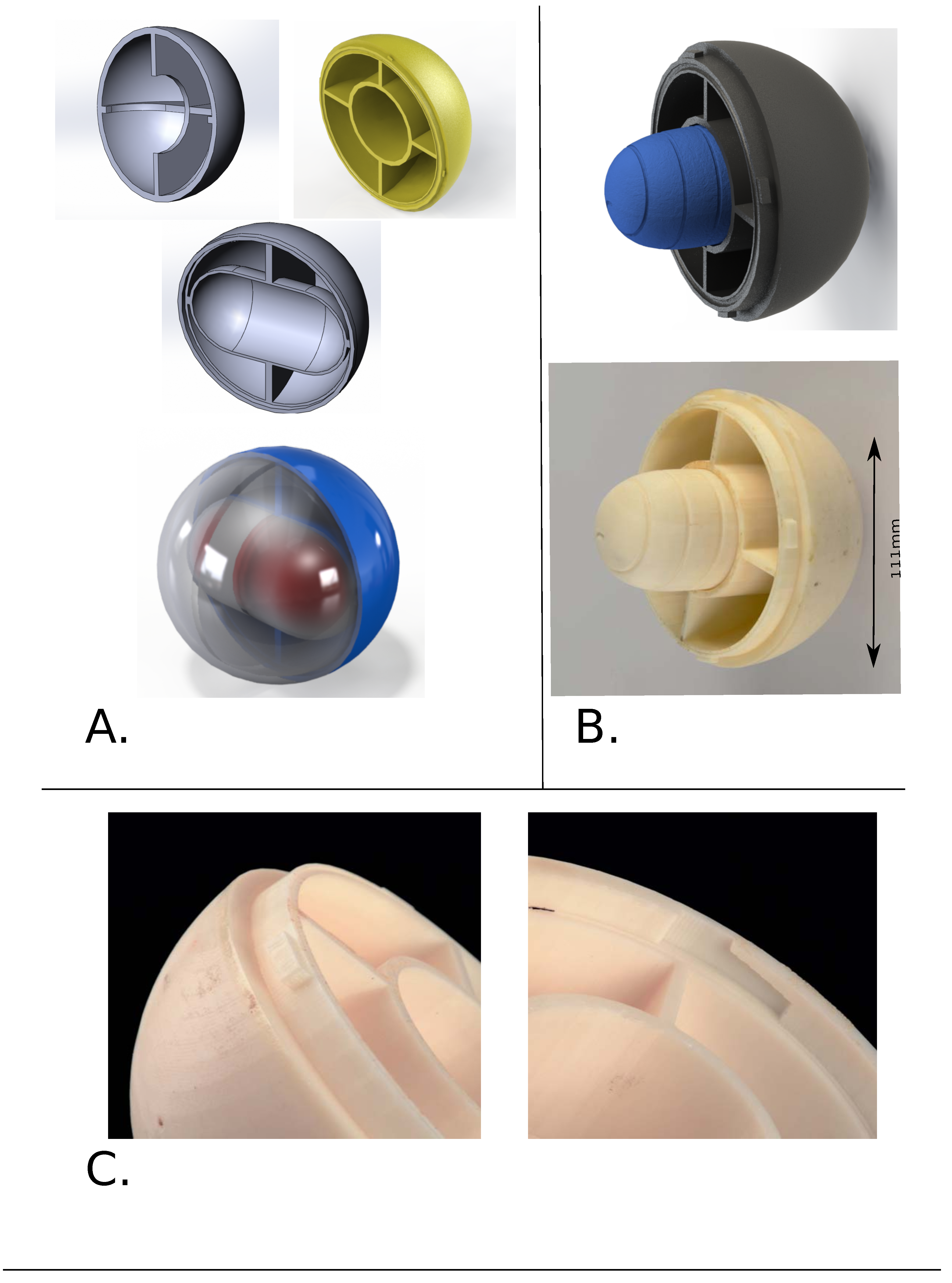
The outer case must also have the internal support required to ensure overall durability (to ensure that the plastic will not crack under sudden stress) and can be used to enhance the water-proofing of the entire system. Durability is achieved by designing strong internal support structures and waterproofing by sculpturing structures, like O-rings, which can be filled with insulating materials (e.g., silicon or rubber). In parallel, the internal structure can be used to control the density of the whole assembly. To achieve this, we constructed the outer case with support structures and void spaces that can be filled with materials of known density that enable control over total mass and density (
Figure 3A).
A challenge is to enable easy access to the sensor when required without risking the case coming open during operation. This requirement is fulfilled by building locking structures into the joints that keep the case firm and rigid when it is closed but enable it to be opened by moving it in a specific way (
Figure 3C).
3.3.2. Cases of Non-Regular Shape
Our ultimate goal is the construction of an outer case to simulate the movement of natural pebbles of variable shapes (hence, the sensor data is as representative as possible). Here, the major concern is to copy effectively the shape of a natural pebble and use it as prototype for the overall case.
For this purpose, the internal case is placed in a modified outer enclosure to generate a more natural shape. There is no single representative shape for any rock type or sedimentary environment [
41], but modern scanning technology allows the replication of any shape.
We model two very different natural stones to illustrate the procedure. The first is a compact blade-shaped stone with medium sphericity (Pebble A in
Figure 4), and the second is a compact platy stone with low sphericity (Pebble B in
Figure 4) [
41]. 3D models of these two cases where generated by a 3D laser scanner (Roland
TM 600 DS [
42]).
Simpler shapes, such as Pebble A, could be represented using simpler input methods, such as those used for the prototypes of the sensors, but this approach is inadequate for capturing the complexity of the pebbles, such as Pebble B. The design for the second case is exclusively based on the 3D scan, as this is the most accurate and fastest procedure.
A basic advantage of this design process is that it is possible to integrate almost directly the internal structure designed for the spherical case (which secures the durability and control of the density), by following simple scaling and integration tools provided by the software.
The above method is very versatile in terms of scaling, since it is possible to construct cases that are based on stones much larger or much smaller than the actual sensor. Accurate scaling can enhance the representativeness of the derived data, because when a representative pebble shape is determined for a specific site, it can be scaled to fit the sensor, no matter how diverse is the sample of stones upon which this decision was based,given that the procedure for deciding the representative shape of the grains for a specific site involves sampling and performing a number of statistical calculations that result in a number of characteristic shapes for the site. For example, in
Figure 4, the 3D representation of Pebble A printed at 1:1 scale for demonstration (
Figure 4B) and the constructed case based on this pebble (
Figure 4B,C) were designed using the same input.
Figure 4 also shows a scaled representation for Pebble B.
Figure 3.
Spherical outer case: (A) Designs for the internal structure of the outer case. The case can be designed to enhance durability (support structures), water-proof performance (O-rings) and density control (voids); (B) Incorporation of the internal case for the G-node (design and photograph); (C) Demonstration of the locking system to make the overall assembly rigid, but not impossible to open.
Figure 4.
Scaled copies of natural stones and representative example case: (
A) 3D designs of natural stones after processing the data from the 3D scanner. Note the differences in angularity and sphericity (Pebble A is blade-shaped with medium sphericity; Pebble B is compact and platy with low sphericity); (
B) Scaled 3D printings of Pebble A (
left) and Pebble B (
right); (
C) Outer case based on Pebble A. The internal structure incorporates the internal case for the G-node. This outer case has a simple internal structure, but more complicated internal designs, such as used for the spherical cases, can be incorporated (
Figure 3).
4. Results and Discussion
4.1. Timing of Development: Technical Considerations
We printed with an HP Designjet
TM 3D printer [
43] using standard, compatible with the printer, PVC plastic. The quality of the printer is crucial for the time of development (3D printing proved to be the most time-consuming part of the whole procedure), as well as for the quality of the final product. This becomes more apparent during the latter stages of the development, where the actual enclosures are produced. As an indication, the printing time for the replicates of the sensors (
Figure 1) (a length of 64 mm for the CM4000, for example) is close to four hours, while the 3D printing of the outer enclosures varies from eight to 20 h, depending upon the thickness, the internal supports and the complexity of the shapes being reproduced.
The time required to produce the 3D designs is highly variable and depends on the experience of the modeller and familiarity with the software. However, a modeller relatively familiar with the principals of Digital Design and commonly used 3D Modelling /Computer Aided Design software can be expected to create a first prototype for a given sensor in less than a week, especially if the outer case is based on a natural pebble or an enclosure that can be scanned with the 3D scanner.
It is important that fast prototyping and 3D printing is possible for other materials besides the ABS plastic that is used for this application [
44]. Moreover, the same design process can be followed to create casts for the creation of cases constructed with different materials (e.g., carbon fibre or metals) that can address the requirements for several applications. The inputs and the initial designs in this case would be manipulated following exactly the same procedure. The only differences would be at the final stage, where the designs used as input from the 3D printer must be modified to represent the exact negatives of the desired enclosure (a process very similar to the one followed in order to enclose accurately the sensors in the internal case).
4.2. Data Coherence: Initial Laboratory Tests
The complete testing of the data generated by sensors constructed as described above is ongoing. Here, we demonstrate how selected design features of the case affect the calibration process of the sensor and can potentially enhance the field deployment of such a system.
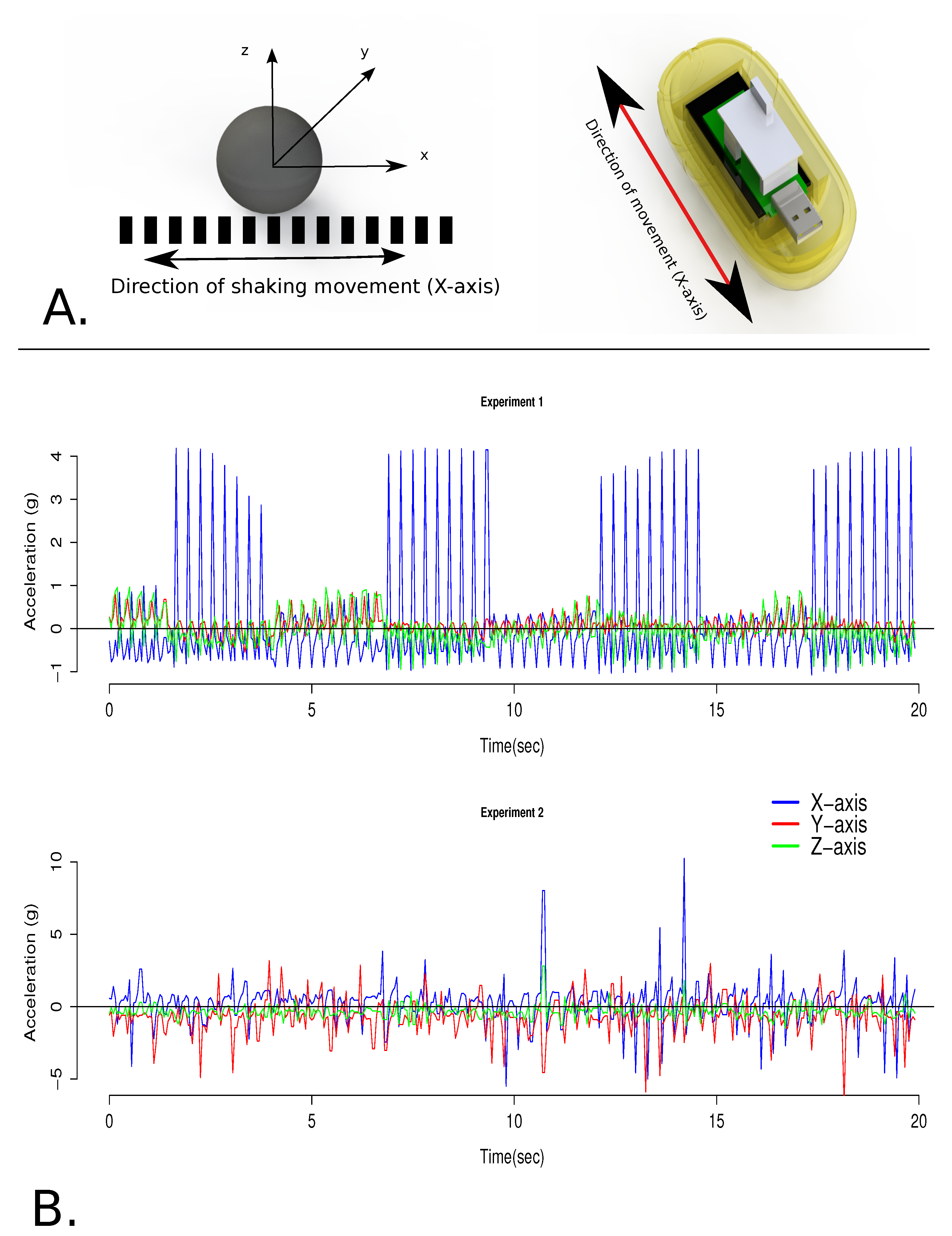
Firstly, the ability of the casing to rigidly fix the sensor in position is critical.
Figure 5 shows the difference between accelerations measured with the same sensor (the G-node) using two different enclosures. The experimental set-up consists of a shaking table moving periodically along one axis and capable of producing a variable acceleration with a known maximum of 4 g. The sensor is firmly attached to monitor the acceleration along the dominant axis (parallel to the movement of the table), as shown in the schematic representation of
Figure 5A. The accelerations recorded in this axis must be significantly greater than those due to the rest of the vibrations produced by the whole shaking movement.
Figure 5.
Experimental comparison between steady and unsteady sensor orientations. (A) Schematic resolution of the 3D orientation of the sensor in relation to the periodic movement of the shaking table. The table creates a range of accelerations up to 4 g. Left: the axes of acceleration in relation to the outer casing. Right: axis of shaking (x-axis) relative to the internal case; (B) Comparison of the raw three-axis acceleration for the two experiments (sampling rate 20 Hz. During Experiment 1, periodic x-axis accelerations reach a maximum of 4.2 g, which significantly exceeds the maxima on the y- and z-axes (0.85 g and 0.96 g, respectively), confirming the direction and magnitude of the dominant process (periodic movement along the x-axis). Experiment 2 was performed without the internal case; hence, sensor orientation changed through time. The maximum acceleration for the x-axis is much larger than that produced by the shaking table ( g). Moreover, the periodic movement is not recorded, and the comparison with the maxima on the other axes (3.18 g and 2.8 g on the y- and z-axes, respectively) is not indicative of the dominant process.
![Jsan 02 00761 g005]()
During the first experiment (
Figure 5B), the sensor was enclosed in the case that was designed following the previously-described procedure. As a result, the sensor was steadily orientated throughout the experiment and was moving as little as possible in relation to the whole case.
Figure 5B shows the recorded acceleration along the three axes during a time period of 20 s at a sampling rate of 20 Hz. The raw signal indicates a dominant periodic impact on the x-axis capable of producing maximum acceleration of 4.2 g, which is significantly greater than the accelerations recorded on the other two axes.
In comparison, for the second experiment, the sensor was enclosed in a case with the same outer shape, but without the internal structure to stabilize the sensor, thus permitting the movement of the sensor within the casing.
Figure 5B shows the results for the same accelerations, time period and sampling frequency as for Experiment 1. The results show how the movement of the sensor inside the case changes its orientation constantly, so that it is difficult to observe the orientation and magnitude of the motion. As a result, the recorded accelerations are inconsistent during the second experiment since: (a) the periodic motion of the shaking table is not recorded; and, more importantly; (b) the relative internal motion of the sensor generates an error as high as 150%, since the maximum acceleration produced from the shaking table is 4 g and, during the second experiment, the measurements for the x-axis have a maximum of 10 g.
4.3. Statistical Analysis
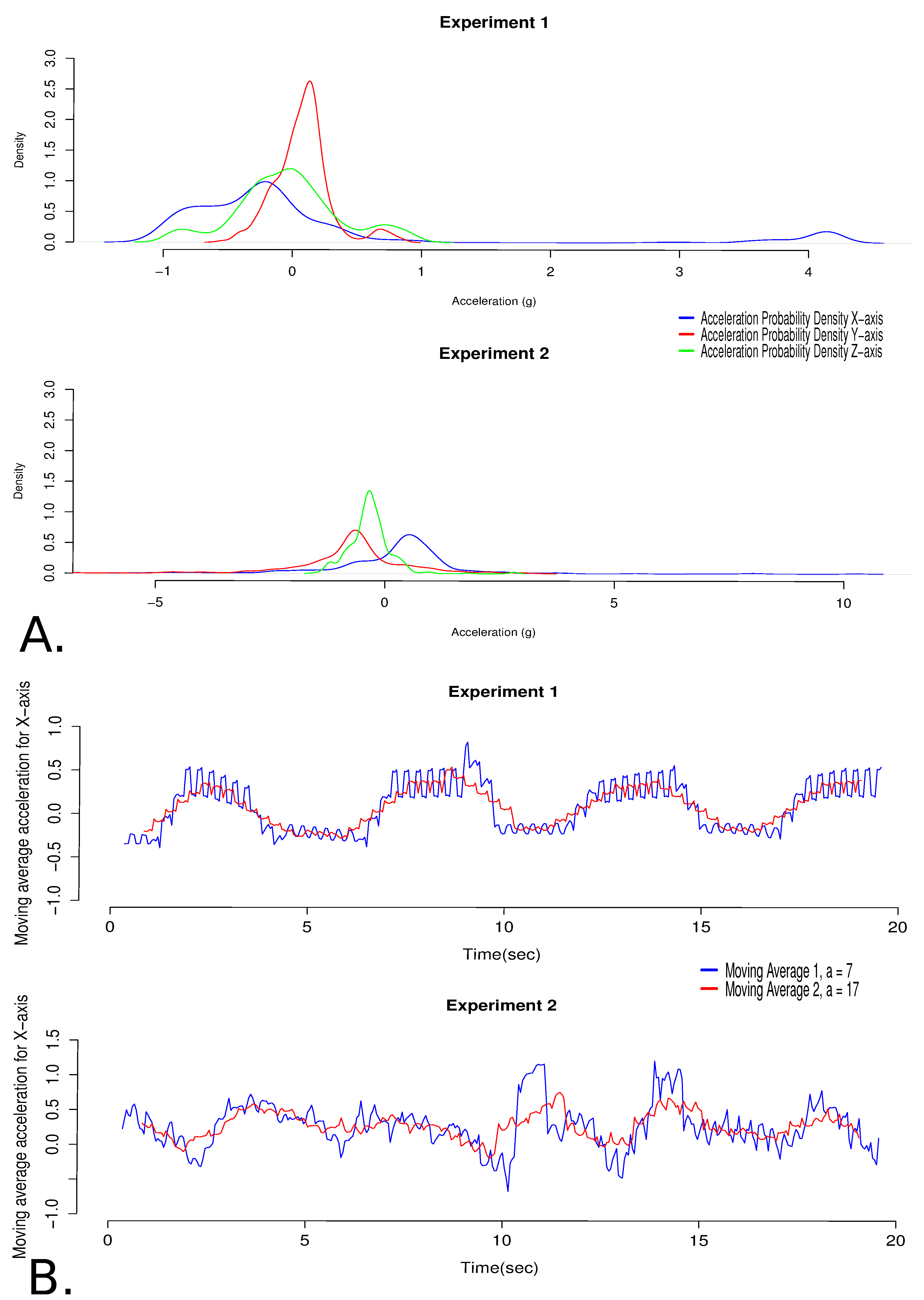
Moving a step further, we demonstrate how misleading the statistical analysis of data from a non-rigid sensor can be. Common practice for time series analysis involves the comparison of the distribution of each measurement and the application of linear filters (smoothing) in order to identify any trends or patterns that drive the monitored process.
Figure 6 shows a statistical comparison between the acceleration signals derived during the two experiments.
4.3.1. Comparison Based on Variability
The first comparison concerns the kernel density of the signals for the three axes (x, y, z). For the first experiment (
Figure 6A), the results reveal similar probability distributions for the accelerations on the y- and z-axes. The mean acceleration is very close to 0 g (0.078 g for the y-axis and −0.02 g for the z-axis), the standard deviation is of the same order (0.21 g and 0.4 g for y and z, respectively), as well as the range ([−0.544,0.856] g for the y-axis and [−0.952,0.960] g for the z-axis).
Interestingly, the probability distribution for acceleration on the x-axis is considerably different. The statistics of this signal reveal a different behaviour (the mean is equal to 0.074 g, with a standard deviation of 1.28 g, and the range is [−1.080,4.208] g). More importantly, the kernel density increases near the value of 4 g, indicating the significance of the maximum values. This peak can be interpreted as an indication of the periodic character of the effect. Overall, these results are representative for the magnitude and the direction of the dominant process, which is movement along the x-axis.
In comparison, the results from the second experiment are not representative. The results reveal similar probability distributions for the accelerations along the y- and x-axes. The mean acceleration is −0.7 g (standard deviation of 1.23 g) for the y-axis and 0.2 g (standard deviation of 1.47 g) for the x-axis, which makes the observation of the dominant process difficult. Moreover, the data give no indication of the periodic movement.
Figure 6.
Statistical comparison of acceleration signals: (A) Kernel densities for acceleration signal (three-axes). Experiment 1 data shows the magnitude of x-axis acceleration as an increase in probability density near 4 g. The unstable signal from Experiment 2 does not give any indication about the dominant process, since the distributions of the three axis signals are statistically similar; (B) Moving Average Smoothing are the caps necessary of x-axis acceleration signals. Linear filters ( and ) retain the periodic pattern during Experiment 1 with an approximate period of 5 s, while for Experiment 2, there is no indication of this behaviour.
4.3.2. Comparison Based on Linear Filtering (Smoothing)
Following the common practice, we applied two moving average filters to the time series of the acceleration signal on the x-axis (where the dominant movement takes place). The averaging factor for the first filter is
and for the second
. The results for the first experiment (
Figure 6B) reveal the seasonal periodic pattern in the time series suggesting an approximate period of 5 s (which is in agreement with the period measured after the analysis of the video recordings of the experiment). On the contrary, the results from the second experiment do not reveal this type of pattern, which is inconsistent, given the movement of the sensor.
4.3.3. Deployment Considerations
While it is unlikely that any sensing system will be constructed without taking into account the error produced by not securing the stability of the sensor inside the casing, our second experiment simulates effectively a situation where a casing fails during operation, a prospect that cannot be excluded in deployments where accelerations on the order of 100 g are possible.
An operator of this sensor is equally likely to receive both of the above signals during real deployment (
Figure 5). Especially in a natural setting where the line-of-sight contact with the system is not guaranteed, the only information about the monitored process is that derived from the statistical analysis of these signals. Taking into account that the known magnitude range of instantaneous measured physical properties can be significantly higher than the range of the derived measurements, both of these signals could appear to be valid and there is no way to identify the error in the second experiment during the statistical analysis. Consequently, it is important to prioritize stable orientation of the sensor in the case and minimization of internal movement during the design process of such a system.
5. Conclusions
Here, we demonstrate a new method for rapid prototyping of sensor enclosures. Focusing on inertial sensors for monitoring motion, the motivation for the development of this method lies in the potential inconsistency of the sensed data if two critical factors are not incorporated in the casing-design criteria: (a) the effect of the physical characteristics of the complete sensor on the movement of the device, hence on the representativeness of the derived data; and (b) the stability of the sensor along with the constant orientation in response to the overall frame of the casing.
We have described a versatile design process that can be adapted to any type of sensor platform and yields casings with pre-determined physical characteristics (such as shape and density). This enables the rapid design of casings for specific applications that will enhance the coherence of the data, since they will be compatible with the monitored environment and the data-acquisition process.
The results concern the application of this method during the development of a new sensor for monitoring river grain dynamics. Given the rapid improvements in the fast prototyping technologies described (which are both enhancing the quality and decreasing the price of the final case product), it is possible to apply this method for large-scale sensing applications.
Finally, we present results from two calibration experiments using an acceleration-impact sensor. The statistical analysis of the results suggests a potential error on the order of 150% in terms of magnitude and complete inconsistency in terms of the directional information about the movement of the sensor when the failure of the case to stabilize the sensor platform is simulated. This result can be considered in the context of remote sensing when no other information is available and the statistical analysis gives no indication about the potential error.
Acknowledgments
The authors thank Ewan Russell for his help during the production of the designs and 3D printed prototypes and cases.
Georgios Maniatis is a PhD student funded by a University of Glasgow Kelvin-Smith Scholarship.
Conflicts of Interest
The authors declare no conflict of interest.
References
- Hart, J.K.; Martinez, K. Environmental sensor networks: A revolution in the earth system science? Earth Sci. Rev. 2006, 78, 177–191. [Google Scholar]
- Corke, B.P.; Wark, T.; Jurdak, R.; Hu, W.; Valencia, P.; Moore, D. Environmental wireless sensor networks. Proc. IEEE 2010, 98, 1903–1917. [Google Scholar] [CrossRef]
- Oliveira, L.M.; Rodrigues, J.J. Wireless sensor networks: A survey on environmental monitoring. J. Commun. 2011, 6, 143–151. [Google Scholar] [CrossRef]
- Benelli, G.; Pozzebon, A.; Bertoni, D.; Sarti, G. An RFID-based toolbox for the study of under- and outside-water movement of pebbles on coarse-grained beaches. IEEE J. Sel. Topics Appl. Earth Observ. Remote Sens. 2012, 5, 1474–1482. [Google Scholar] [CrossRef]
- Werner-Allen, G.; Lorincz, K.; Welsh, M.; Johnson, J.; Lees, J. Deploying a wireless sensor network on an active volcano. IEEE Inter. Comput. Sens. Netw. Appl. 2006, 10, 18–25. [Google Scholar] [CrossRef]
- Martinez, K.; Hart, J.K.; Ong, R. Deploying A Wireless Sensor Network in Iceland. In GeoSensor Networks; Springer: Berlin, Germany, 2009; pp. 131–137. [Google Scholar]
- Pedersen, L.; Bualat, M.; Kunz, C.; Lee, S.; Sargent, R.; Washington, R.; Wright, A. Instrument Deployment for Mars Rovers. In Proceedings of the 2003 IEEE International Conference on Robotics and Automation (ICRA 2003), Taipei, Taiwan, 14–19 September 2003; pp. 2535–2542.
- Whipple, K.X.; Tucker, G.E. Implications of sediment-flux-dependent river incision models for landscape evolution. J. Geophys. Res. 2002, 107(B2), ETG 3-1–ETG 3-20. [Google Scholar] [CrossRef]
- Hassan, M.A.; Ergenzinger, P. Use of Tracers in Fluvial Geomorphology. In Tools in Fluvial Geomorphology; John Wiley & Sons, Ltd: Hoboken, NJ, USA, 2005; pp. 397–423. [Google Scholar]
- Habersack, H.M. Use of radio-tracking techniques in bed load transport investigations. In Proceedings of Erosion and Sediment Transport Measurement in Rivers: Technological and Methodological Advances: Workshop, Oslo, Norway, 19–21 June 2002; pp. 172–180.
- Allan, J.C.; Hart, R.; Tranquili, J.V. The use of Passive Integrated Transponder (PIT) tags to trace cobble transport in a mixed sand-and-gravel beach on the high-energy Oregon coast, USA. Mar. Geol. 2006, 232, 63–86. [Google Scholar] [CrossRef]
- Furbish, D.J.; Ball, A.E.; Schmeeckle, M.W. A probabilistic description of the bed load sediment flux: 4. Fickian diffusion at low transport rates. J. Geophys. Res. 2012, 117, F03034. [Google Scholar] [CrossRef]
- McEwan, I.; Habersack, H.; Heald, J. Discrete Particle Modelling and Active Tracers: New Techniques for Studying Sediment Transport as a Lagrangian Phenomenon. In Gravel-Bed Rivers V; New Zealand Hydrological Society: Wellington, New Zealand, 2001; pp. 339–360. [Google Scholar]
- Demir, T. The Influence of Particle Shape on Bedload Transport in Coarse-Bed River Channels. Ph.D. Thesis, Durham University, Durham, UK, 2000. [Google Scholar]
- Ergenzinger, P.; Jupner, R. Using COSSY (CObble Satellite SYstem ) for measuring the effects of lift and drag forces. In Erosion and Sediment Transport Monitoring Programmes in River Basins; IAHS Press: Oxford, UK, 1992; pp. 41–50. [Google Scholar]
- Krumbein, W.C. Measurement and geological significance of shape and roundness of sedimentary particles. J. Sediment. Res. 1941, 11, 64–72. [Google Scholar] [CrossRef]
- Carling, P.; Kelsey, A.; Glaister, M. Effect of Bed Roughness, Particle Shape and Orientation on Initial Motion Criteria. In Dynamics of Gravel Bed Rivers; John Wiley and Sons: Chichester, UK, 1992; pp. 24–39. [Google Scholar]
- Wiberg, P.L.; Smith, J.D. Model for calculating bed load transport of sediment. J. Hydraul. Eng. 1989, 115, 101–123. [Google Scholar] [CrossRef]
- Hodge, R.A.; Hoey, T.B.; Sklar, L.S. Bed load transport in bedrock rivers: The role of sediment cover in grain entrainment, translation, and deposition. J. Geophys. Res. 2011, 116, 1–19. [Google Scholar] [CrossRef]
- Sear, D.; Lee, M.; Collins, M.; Carling, P. The Intelligent Pebble: A New Technology for Tracking Particle Movements in Fluvial and Littoral Environments. In Proceedings of Erosion and Sediment Transport Measurement: Technological and Methodological Advances Workshop, Oslo, Norway, 19–21 June 2002; pp. 19–21.
- Spazzapan, M.; Petrovčič, J.; Mikoš, M. New tracer for monitoring dynamics of sediment transport in turbulent flows. Acta Hydrotech. 2004, 22, 135–148. [Google Scholar]
- Abeywardana, D.K.; Hu, A.P.; Kularatna, N. Design Enhancements of the Smart Sediment Particle for Riverbed Transport Monitoring. In Proceedings of 4th IEEE Conference on Industrial Electronics and Applications, Xi’an, China, 25–28 May 2009; pp. 336–341.
- Abeywardana, D.K.; Hu, A.P.; Kularatna, N. IPT Charged Wireless Sensor Module for River Sedimentation Detection. In Proceedings of 2012 IEEE Sensors Applications Symposium (SAS 2012), Deauville, France, 11–13 September 2012; pp. 1–5.
- Frank, D.P.; Foster, D.L.; Kao, P.C.Y.M. In-Situ Measurements within Mobile Bed Layers with Electronic Pebbles. In Proceedings of American Geophysical Union Conference, San Francisco, CA, USA, 9–15 December 2012; p. 3.
- Rickenmann, D.; McArdell, B. Continuous measurement of sediment transport in the Erlenbach stream using piezoelectric bedload impact sensors. Earth Surf. Process. Landf. 2007, 32, 1362–1378. [Google Scholar] [CrossRef]
- Vatne, G.; Naas, O.T.; Skarholen, T.; Beylich, A.A.; Berthling, I. Bed load transport in a steep snowmelt-dominated mountain stream as inferred from impact sensors. Nor. Geogr. Tidsskr. Nor. J. Geogr. 2008, 62, 66–74. [Google Scholar] [CrossRef]
- Nichols, M. A radio frequency identification system for monitoring coarse sediment particle displacement. Appl. Eng. Agric. 2004, 20, 783–787. [Google Scholar] [CrossRef]
- Bradley, D.N.; Tucker, G.E. Measuring gravel transport and dispersion in a mountain river using passive radio tracers. Earth Surf. Process, Landf. 2012, 37, 1034–1045. [Google Scholar] [CrossRef]
- Liedermann, M.; Tritthart, M.; Habersack, H. Particle path characteristics at the large gravel-bed river Danube: Results from a tracer study and numerical modelling. Earth Surf. Process. Landf. 2012, 38, 512–522. [Google Scholar] [CrossRef]
- Heidemann, J.; Stojanovic, M.; Zorzi, M. Underwater sensor networks: Applications, advances and challenges. Philos. Trans. R. Soc. A Math. Phys. Eng. Sci. 2012, 370, 158–175. [Google Scholar] [CrossRef] [PubMed]
- Fiorelli, E.; Leonard, N.; Bhatta, P.; Paley, D.; Bachmayer, R.; Fratantoni, D. Multi-AUV control and adaptive sampling in monterey bay. IEEE J. Ocean. Eng. 2006, 31, 935–948. [Google Scholar] [CrossRef]
- Detweiler, C.; Doniec, M.; Vasilescu, I.; Basha, E.; Rus, D. Autonomous Depth Adjustment for Underwater Sensor Networks. In Proceedings of the Fifth ACM International Workshop on UnderWater Networks, New York, NY, USA, 30 September–1 October 2010; pp. 12:1–12:4.
- Hanrahan, G.; Patil, D.G.; Wang, J. Electrochemical sensors for environmental monitoring: Design, development and applications. J. Environ. Monitor. 2004, 6, 657–664. [Google Scholar]
- Akyildiz, I.F.; Vuran, M.C. Wireless Underwater Sensor Networks. In Wireless Sensor Networks; John Wiley & Sons: Hoboken, NJ, USA, 2010; pp. 399–442. [Google Scholar]
- Delauney, L.; Compere, C.; Lehaitre, M. Biofouling protection for marine environmental sensors. Ocean. Sci. 2010, 6, 503–511. [Google Scholar] [CrossRef]
- AdvanticSys, CM4000 Mote Webpage. Avaiable online: http://www.advanticsys.com/shop/mtmcm4000msp-p-8.html (accessed on 28 November 2013).
- AdvanticSys, CO1000 Sensor-Board Webpage. Avaiable online: http://www.advanticsys.com/shop/mtsco1000-p-17.html (accessed on 28 November 2013).
- SOWNET Technologies, G-Node Mote Webpage. Avaiable online: http://www.sownet.nl/index.php/products/gnode (accessed on 28 November 2013).
- Analogue Devices, ADXL-345 Digital Accelerometer Webpage and Datasheet. Avaiable online: http://www.analog.com/en/mems-sensors/mems-inertial-sensors/adxl345/products/product.html (accessed on 28 November 2013).
- Dassault Systèmes, SolidWorks Software Webpage. Avaiable online: http://www.solidworks.com (accessed on 28 November 2013).
- Benn, D.I.; Ballantyne, C.K. The description and representation of particle shape. Earth Surf. Process. Landf. 1993, 18, 665–672. [Google Scholar] [CrossRef]
- Roland 3D-Scanners Webpage. Avaiable online: http://www.rolanddga.com/products/scanners/lpx600/ (accessed on 28 November 2013).
- Hp Designjet 3D Printer Webpage. Avaiable online: http://www.hp3dprinting.co.uk/hp-designjet-color-3d-printer.html (accessed on 28 November 2013).
- Lipson, H.; Kurman, M. Fabricated: The New World of 3D Printing; John Wiley & Sons: Hoboken, NJ, USA, 2013. [Google Scholar]
© 2013 by the authors; licensee MDPI, Basel, Switzerland. This article is an open access article distributed under the terms and conditions of the Creative Commons Attribution license (http://creativecommons.org/licenses/by/3.0/).
