Enhanced Distributed Dynamic Skyline Query for Wireless Sensor Networks

Abstract

Dynamic skyline query is one of the most popular and significant variants of skyline query in the field of multi-criteria decision-making. However, designing a distributed dynamic skyline query possesses greater challenge, especially for the distributed data centric storage within wireless sensor networks (WSNs). In this paper, a novel Enhanced Distributed Dynamic Skyline (EDDS) approach is proposed and implemented in Disk Based Data Centric Storage (DBDCS) architecture. DBDCS is an adaptation of magnetic disk storage platter consisting tracks and sectors. In DBDCS, the disc track and sector analogy is used to map data locations. A distance based indexing method is used for storing and querying multi-dimensional similar data. EDDS applies a threshold based hierarchical approach, which uses temporal correlation among sectors and sector segments to calculate a dynamic skyline. The efficiency and effectiveness of EDDS has been evaluated in terms of latency, energy consumption and accuracy through a simulation model developed in Castalia.

1. Introduction

WSNs have successfully been validated as a very economic and effective platform for monitoring diverse physical environments from remote locations. Various types of query techniques have been developed over WSNs including min-max [1], top-k [2,3] and skyline [4]. Skyline and its variants such as traditional skyline [5] and dynamic skyline [6,7,8] have been applied in many multiple criteria decision making applications. Traditional skyline (TS) retrieves all of the points, which are not dominated by others, from a set of points [9]. Given a dataset X, a point x₁ dominates x₂, if x₁ is not worse than x₂ for each dimension $i\in l$ (i.e., x₁[i] ≤ x₂[i]), and x₁ is better than x₂ for at least one dimension $m\in l$ (x₁[m] < x₂[m]). 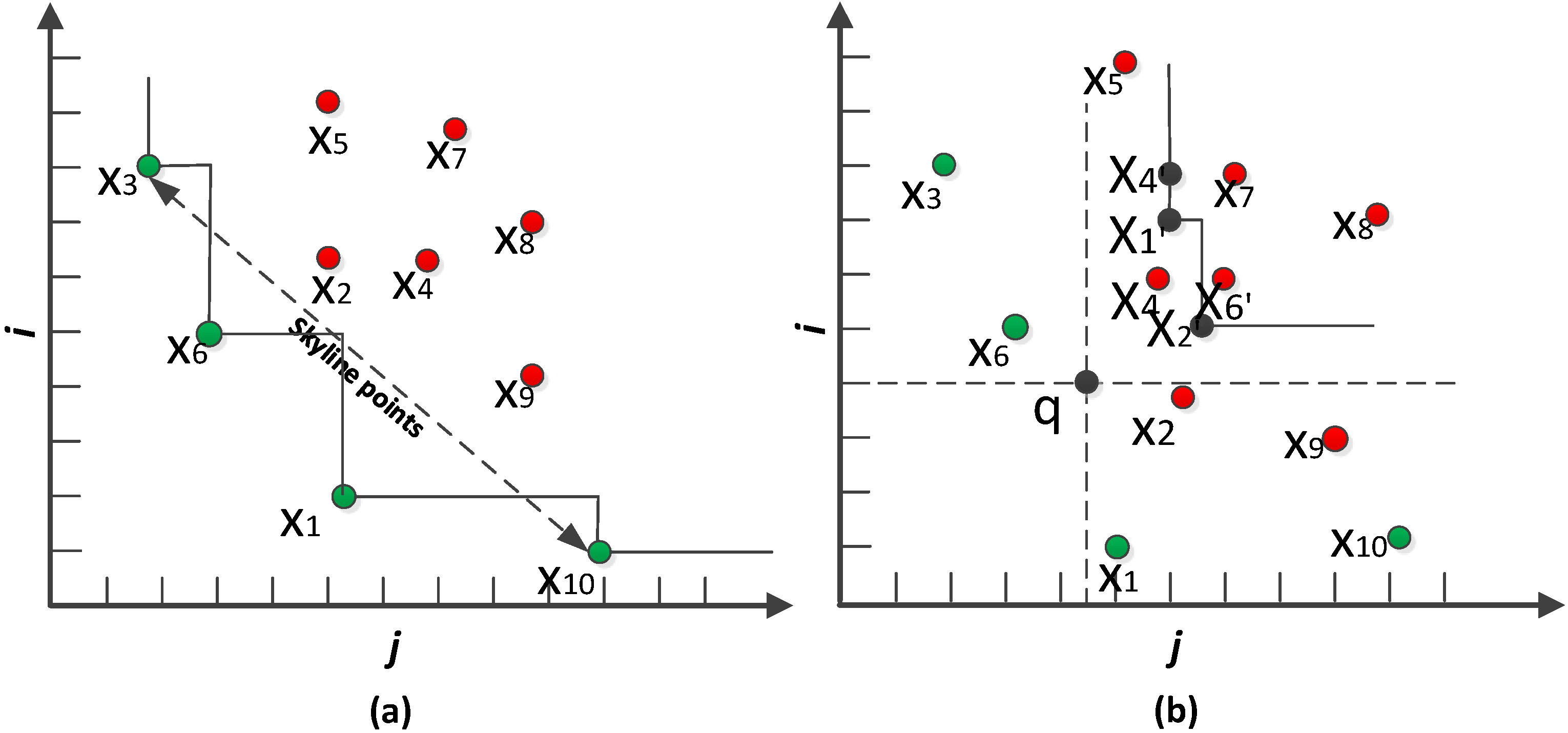Figure 1a shows an example, where each point is drawn taking two dimensions i and j as coordinators; points x₁, x₃, x₆ and x₁₀ are in the skyline set considering that a point with the least value for each dimension is desirable.

Dynamic skyline (DS) retrieves a set of points that are not dynamically dominated by others with respect to a data point q denoted by DS (q, X)) [10]. A point x₁ dynamically dominates x₂ with respect to q if for each dimension in $i\in l$, $\left|x_1\left[i\right]-q\left[i\right]\right|\le \left|x_2\left[i\right]-q\left[i\right]\right|$ and for at least one dimension in $m\in l$, $\left|x_1\left[m\right]-q\left[m\right]\right|<\left|x_2\left[m\right]-q\left[m\right]\right|$. In Figure 1b, points x₁, x₂ and x₄ are the dynamic skyline points of q. Each point x_i = (x_i[j], x_i[i]) is transformed to x_i′ = (x_i[j]−q[j], x_i[i]−q[i]).

Figure 1. (a) TS and (b) DS (q, X).

Figure 1. (a) TS and (b) DS (q, X).

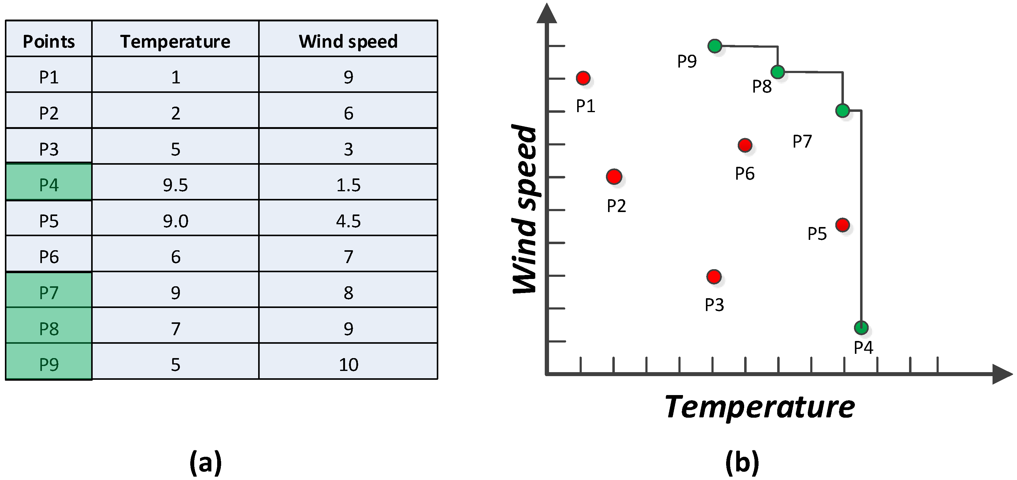
Skyline query is very useful in multi-preference analysis and decision making for environmental monitoring applications. For example, in a WSN deployed in a forest with each sensor node sensing temperature and wind speed, it is possible to build a fast and energy efficient forest fire detection method [11] by concentrating on places with high temperature or fast wind speed, or both. To illustrate the idea of dominance relations in this scenario, consider the readings in the two-dimensional attribute space shown in Figure 2 depicting a typical example of ranking objects by more than one criterion. Figure 2a lists nine records received from nine corresponding sensor nodes deployed in different places and their values. Figure 2b depicts the representation in a 2D space. Places P₁, P₂, P₃, P₅, and P₆ are all dominated by other points so the skyline query returns the points that are not dominated by any other points. Consider the point P₅ that is dominated by P₇, as it has a higher wind speed than P₅ though both have the same temperature. The skyline query only retrieves the dominant places in terms of higher temperature and wind speed. The skyline query will not exhibit any place with lower temperature and wind speed once it is dominated by a location with higher values. Therefore, the result set of the skyline query consists of {P₄, P₇, P₈, P₉}, which are indicators of dangerous places that need special attention.

Figure 2. (a) Skyline of sensor readings, (b) Representation of sensor readings in 2D space [11].

Figure 2. (a) Skyline of sensor readings, (b) Representation of sensor readings in 2D space [11].

Another example that demonstrates the usefulness of DS can be found when monitoring the air pollution in a region of interest. A high concentration of CO or SO₂, or both, can be a strong indication that the location is highly polluted. An environmental scientist can issue a dynamic skyline query for CO and SO₂ levels to monitor the air pollution surrounding a particular region of interest.

DS query processing over moving objects is also very useful for numerous applications, such as location-aware computing, object tracking and monitoring, virtual environments, uncertain data stream, computer games, visualization, etc.

Although the skyline query approach has potential for use in WSN applications, it faces challenges because of high processing complexity and cost related with updating the results. The main contributors to the high cost are the data access cost from storage locations and the processing cost while executing the user specified query for a dominance check. It is important to note that search efficiency and update criteria are two key requirements of skyline query processing and skyline result maintenance.

Data-Centric Storage (DCS) [12,13], an alternate to External Storage (ES) and Local Storage (LS), is considered to be a promising and efficient storage and search mechanism. There has been a growing interest in understanding and optimizing WSN DCS schemes in recent years, where a various number of query mechanisms such as point query, range query, similarity searching, top-k query and skyline query can be applied in a consolidated framework. As part of developing such consolidated framework, this paper proposes a threshold based hierarchical approach, which uses temporal correlation among the sectors and sector segments to calculate DS in a region of interest. To our knowledge, this is the first practical demonstration of DS in DCS of WSN in current state-of-the-art.

In this paper, first a novel tree building algorithm is incorporated so that each head node of a cluster could construct a tree with itself as a root. This allows exertion of three core operations such as Tree Propagation, Regular Update and Triggered Query from any head node with a particular range. The performance of the proposed model is analyzed by framing and implementing it in a distributed information delivery service running one or more applications in a WSN. In this service, a set of producer and consumer nodes exchange information by relaying packets through neighboring clusters for each application. This phenomenon is facilitated by a DCS [14] architecture, also referred to as DBDCS (Section 3.1). DBDCS is an adaptation of the magnetic disk storage platter consisting of tracks and sectors [15,16]. In DBDCS, each application uses a disc track and sector analogy to map data locations and uses distance based indexing method for storing and querying multi-dimensional similar data. The member nodes in each cluster report the sensed event to their associated head node, which aggregates the received events at the end of each epoch. The aggregated event is hashed to produce a hash key, which is mapped from a one dimensional domain into a metric space [17] (Section 3.3).

The remainder of this paper is structured as follows: Section 2 provides an overview of the related work in the literature. Network architecture, data processing and mapping, insertion and skyline querying are illustrated in Section 3. This is followed by the simulation results and performance evaluation of EDDS presented in Section 4. The paper is concluded in Section 5.

2. Related Work

According to the current state-of-the-art, skyline operator in database community was first introduced by Borzsonyi et al. [5]. In their work, they proposed the solution based on block nested loop (BNL) and divide-and-conquer (D & C). Inspired by BNL, Chomicki et al. [18] and Godfrey et al. [19] proposed two variants of BNL named sort-filter-skylines (SFS) and linear elimination sort for skyline (LESS), respectively. Later, two progressive processing algorithms such as Bitmap and Index were proposed by Tan et al. [20]. Nearest neighbor (NN) method and its variant NN with branch-and-bound (BB) were later presented by Kossman et al. [21] and Papadias et al. [22], respectively. However, these approaches are mainly suitable for centralized environments with high computational and energy resources and thus inappropriate for WSN environments.

A filter-based distributed algorithm for skyline evaluation and maintenance in WSN is proposed by Liang et al. [23]. Each sensor node uses a greedy algorithm to compute a local skyline certificate, which is a subset of the local skyline and forwards it to its parent. The parent or non-leaf node calculates the certificate based on a set of local skyline points plus the certificate received from child nodes. Following this process, the root calculates the set of skyline points, which is used as a Global Skyline Filter (GSF) or global certificate. The root broadcasts the global certificate followed by a simple merge-based algorithm to filter out the points from transmissions that cannot utilize the certificate. An energy efficient Sliding Window Skyline Monitoring Algorithm (SWSMA) is proposed in [24] to continuously maintain sliding window skylines over WSN. It reduces the amount of data transferred and reduces energy consumption, as a consequence, by devising two filter based algorithms: (1) Single point filter based algorithm referred to as a Tuple Filter (TF); and (2) Grid Filter (GF) based algorithm. Chen et al. [25] proposed two evaluation algorithms for finding the skyline points on a dataset progressively. The dataset is first partitioned into disjoint subsets. Then skyline points are returned through the examination of each subset progressively using discovered skyline points to filter out the unlikely skyline points from transmission. However, the features of DCS have not been considered in these approaches and thus direct implication of them in DCS is not suitable.

Song et al. [26] propose a skyline query processing algorithm exploiting the key features of DCS. The algorithm processes a query in three stages on the basis of four assumptions: (1) choice of DCS framework is limited to KDDCS [27], GDCS [28] and DIM [29]; (2) all nodes are identified by unique ID; (3) each node knows the geographic location of its own and its neighbor nodes; and (4) each node knows the range of data stored in its neighbor nodes. In the first stage, the base station locates the Start Node (SN) where the query is to commence. In the second stage, SN creates a Skyline Query Message (SQM) and propagates the SQM to neighbor nodes to search for Candidate Nodes (CNs) where candidate data for the query are stored. This SQM transmission process is repeated until the complete candidate results are found. In the third and final stage BS generates a final query result from its gathered candidate dataset. The aforementioned assumptions made in this work are particularly expensive in a distributed environment like WSN especially DCS framework.

Su et al. [30] proposed an algorithm, known as Skyline Sensor Algorithm (SkySensor), in a customized DCS method in order to collect and store all sensor readings and retrieve skyline results efficiently from the network. The major disadvantages of SkySensor are: (1) SkySensor needs increased effort from an application designer who has to write the center location of each cluster in such a way that no two clusters overlap; (2) number of clusters in a sensor network depends on the number of attributes of a tuple, therefore, an active sensor and actuator network, with higher rate of data generation and a lower number of attributes leads to high concentration of data in a small portion of the network which creates congestion and a hot spot around the cluster and limits the ultimate goal or advantage of DCS; and (3) in the case of resilience to node failure, an inefficient and old technique referred to as local replication is used, which is expected to incur high storage cost and increased data loss during a node group failure.

Based on the above discussion, it is obvious that none of the work from the current literature has implemented DS in WSN, especially in DCS. It consumes great effort in pre-processing, such as gathering the local skylines of all sensors, mapping all detected data of the entire network (both inflow and outflow). The overall process is overwhelmed with higher overheads and complexity if the researcher or analysts are interested in a particular region. In this paper, a threshold based hierarchical DS approach is proposed and implemented using the temporal correlation among the sectors and sector segments. This allows reducing the transmission cost in a greater aspect and facilitates finding skyline points from both entire network and a particular region of interest.

3. Basic System Design

In this section, at first, we briefly discuss the DBDCS network architecture that has been used for testing our proposed EDDS approach. Definition of skyline is restated in Section 3.2 in terms of metric based searching. This is followed by the discussion of data processing, mapping and insertion technique in Section 3.3 and Section 3.4. Finally, we have presented the EDDS approach in Section 3.5.

3.1. Network Architecture

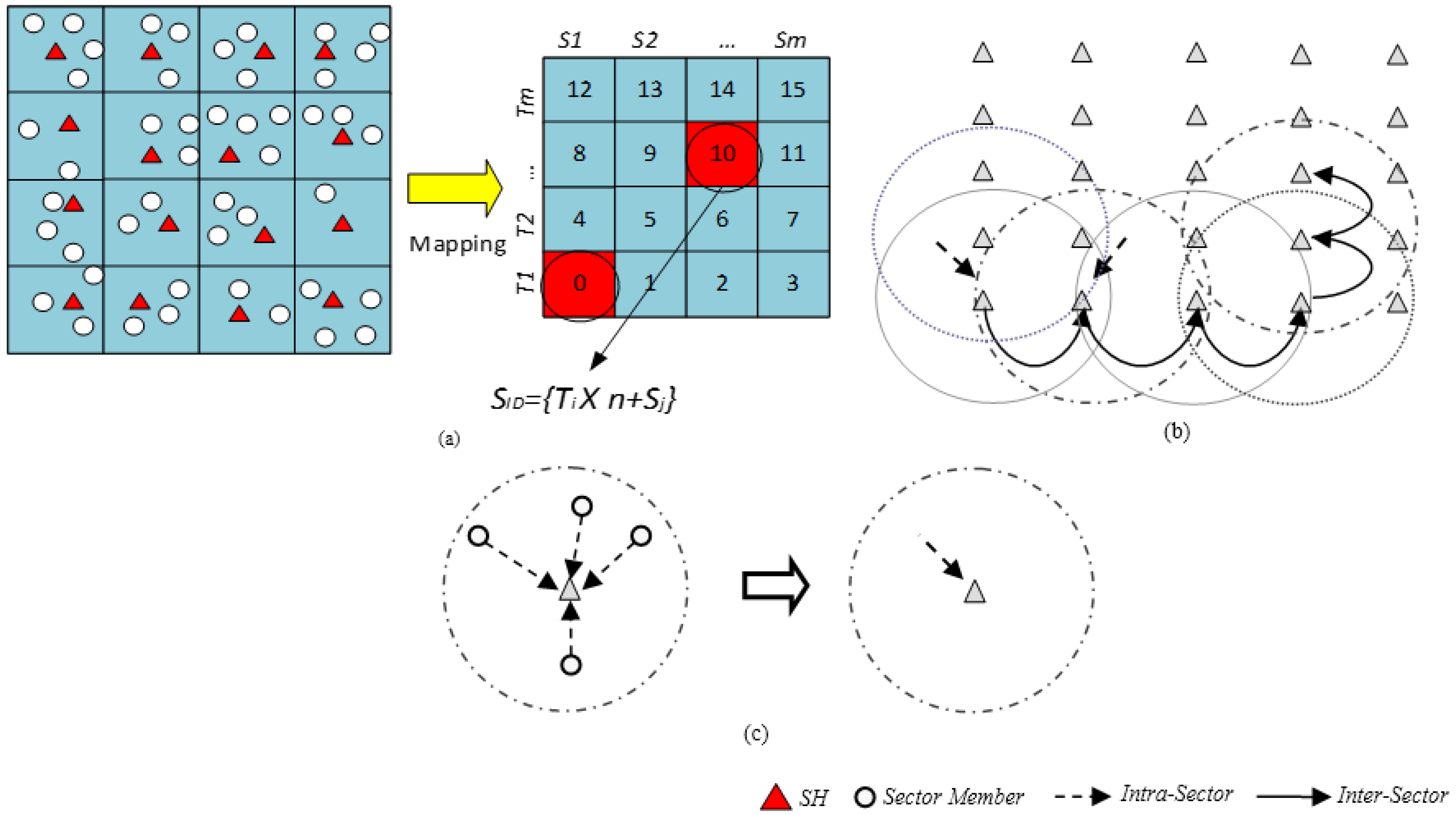
The surface/platter of a magnetic disk storage device consisting of tracks and sectors provides an interesting approach that may be applied to a large scale WSN. This assumption led to the Disk Based Data Centric Storage (DBDCS) architecture, as shown in Figure 3a, dividing the rectangular field into a matrix of storage cells (referred to as a sector) where row and column represent track T_i and sector S_j, respectively. The physical deployment is mapped to a m x n matrix, where m is the number of tracks and n is the number sectors for each track. Hence, the nodes in the network are divided into S(mxn) sectors, each comprising a Sector Head (SH) and sector members that communicate via one hop to the SH (see Figure 3c), where $S{H}_i\in \left[\mathrm{1..}S\right]$. Each node is configured to be aware of the deployment layout by knowing: (1) each SH is assigned with the sector number as a virtual address and node id; and (2) all member nodes know their own node id and number of tracks (m) and sectors (n) of the network field. As shown in Figure 3b, the intra-sector communication (i.e., communication from sector members to SH or vice-versa) is constrained to one hop while inter-sector transmission is multi-hop. For simplification, the sensor nodes inside each sector are not shown explicitly in Figure 3b. Instead, an aggregated link (see Figure 3c) is shown to represent the total traffic from member nodes to head node.

Figure 3. (a) DBDCS Mapping; (b) inter-sector communication; and (c) intra-sector member node to head node communication

Figure 3. (a) DBDCS Mapping; (b) inter-sector communication; and (c) intra-sector member node to head node communication

3.2. Skyline Definition with Metric-Based Searching

Metric space M can be defined as a pair M = (D, d), where D is the domain of objects and d is the distance function—d: D × D ➔ R satisfying the following constraints (Equation (1)) for all objects $a,b,c\in D$:

$$\begin{array}{cc}\hfill d\left(a,b\right)\ge 0\hfill & (\mathrm{non}-\mathrm{negativity})\hfill \\ \hfill d\left(a,b\right)=0\hfill & \left(\mathrm{identity}\right)\hfill \\ \hfill d(a,b)=d(b,a)\hfill & \left(\mathrm{symmetry}\right)\hfill \\ \hfill d(a,c)\le d(a,b)+d(b,c)\hfill & \left(\text{triangle inequality}\right)\hfill \end{array}$$

(1)

In this metric space, considering that smaller values are preferable to larger ones for a set of l-dimensional data, the dynamic skyline query result set can be defined as:

Skyline(q, r):

$$X=\left\{\begin{array}{l}{\forall }_i\in \left[1,l\right],a,b\in I|a(i)\le b(i)\hspace{1em}\hspace{1em}and\\ {\exists }_i\in [1,l],a(i)<b(i)\hspace{1em}\hspace{1em}and\\ d\left(q,a\right)\le r\end{array}\right\}$$

(2)

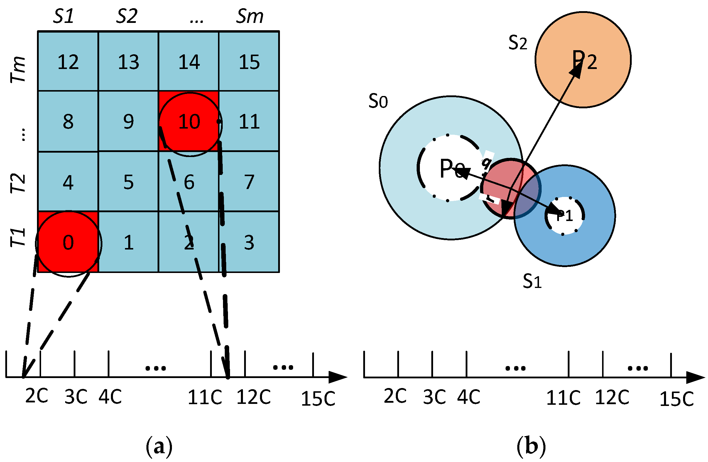
In Equation (2), q denotes the query point, a(i) denotes the value of the ith attribute of an object and r defines the range of the region of interest. The data space is divided into S sectors with a pivot point, denoted by P_i, for each sector S_i. The iDistance key for an object $x\in D$ can be defined as (Figure 4a, Equation (3)):

$$iDist\left(x\right)=d\left(P_i,x\right)+i\cdot c$$

(3)

In Equation (3), c is the separating constant for individual sectors. Given $q\in D$, the region of interest with radius r can be defined as (Figure 4b, Equation (4)):

$$r=\left[d\left(P_i,q\right)+i\cdot c-r,d\left(P_i,q\right)+i\cdot c+r\right]$$

(4)

Figure 4. (a) Data mapping; and (b) range query example.

Figure 4. (a) Data mapping; and (b) range query example.

3.3. Data Processing and Mapping

A sensed event E can be defined by an l- dimensional tuple, (A₁, A₂, A₃, … A_l) where $A_g,{\forall }_g\in \left[1,l\right]$ denotes the gth attribute and $D_{Ag}$ is the domain of attribute A_g. Each member node of a sector transmits the sensed event as an l-tuple ${\langle v_{i1},v_{i2},\mathrm{......},v_{il}\rangle }_k$, where $1\le i\le M_k$, M_k is the total number of member nodes in kth sector and v_ij denotes the value of the jth attribute received from ith node of kth sector. A SH node after collecting tuples from all the member nodes aggregates them at the end of each epoch before finding the mapping for the target SH.

Hence, after aggregation at epoch t

$${\mathrm{E}}_{\mathrm{k}}\left(\text{Agg}\right(t\left)\right)={\displaystyle \underset{{\text{Agg}}_{\mathrm{i}=1}}{\overset{M_k}{\int }}\langle v_{i1},v_{i2},\mathrm{......},v_{il}\rangle \left(t\right)}$$

(5.1)

$$=\langle {\psi }_1,{\psi }_2,\mathrm{.......},{\psi }_l\rangle \left(t\right)$$

(5.2)

Here,

$${\psi }_j=\left\{{\max }_{i=1}^{M_k}{v}_{ij},{\min }_{i=1}^{M_k}{v}_{ij},av{g}_{i=1}^{M_k}\right\},j\in \left[1,l\right],k\in \left[1,S\right]$$

(6)

In Equation (6), M_k denotes the number of member nodes in kth sector. It is assumed that all attribute’s aggregated values of ${\psi }_i$ have been normalized to be between 0 and 1. As shown in Table 1, weights have been assigned to different attributes based on their importance in the event description. Hence, an attribute with higher weight has higher influence in deciding the similarity among events.

Table 1. Weight settings.

Attribute	Weight
A1	w1
A2	w2
....	....
Al	wl

Table 1. Weight settings.

Attribute	Weight
A1	w1
A2	w2
....	....
Al	wl

3.3.1. Pivot Point Generation

$${\alpha }_{\min }={\displaystyle \sum _{i=1}^l\left(\left(\raisebox{1ex}{${{\rm A}}_{i\left(\min \right)}$}\!\left/ \!\raisebox{-1ex}{${{\rm A}}_{i\left(\max \right)}$}\right.\right)\times w_i\right)}$$

(7.1)

$${\alpha }_{\max }={\displaystyle \sum _{i=1}^l\left(\left(\raisebox{1ex}{${{\rm A}}_{i\left(\max \right)}$}\!\left/ \!\raisebox{-1ex}{${{\rm A}}_{i\left(\max \right)}$}\right.\right)\times w_i\right)}$$

(7.2)

$$\beta ={\displaystyle \sum _{i=1}^l\left(\left(\raisebox{1ex}{${{\rm A}}_{i\left(avg\right)}$}\!\left/ \!\raisebox{-1ex}{${{\rm A}}_{i\left(\max \right)}$}\right.\right)\times w_i\right)}$$

(7.3)

$$\delta ={\displaystyle \sum _{i=1}^l\left(\left(\raisebox{1ex}{${{\rm A}}_{i\left(\theta \right)}$}\!\left/ \!\raisebox{-1ex}{${{\rm A}}_{i\left(\max \right)}$}\right.\right)\times w_i\right)}$$

(7.4)

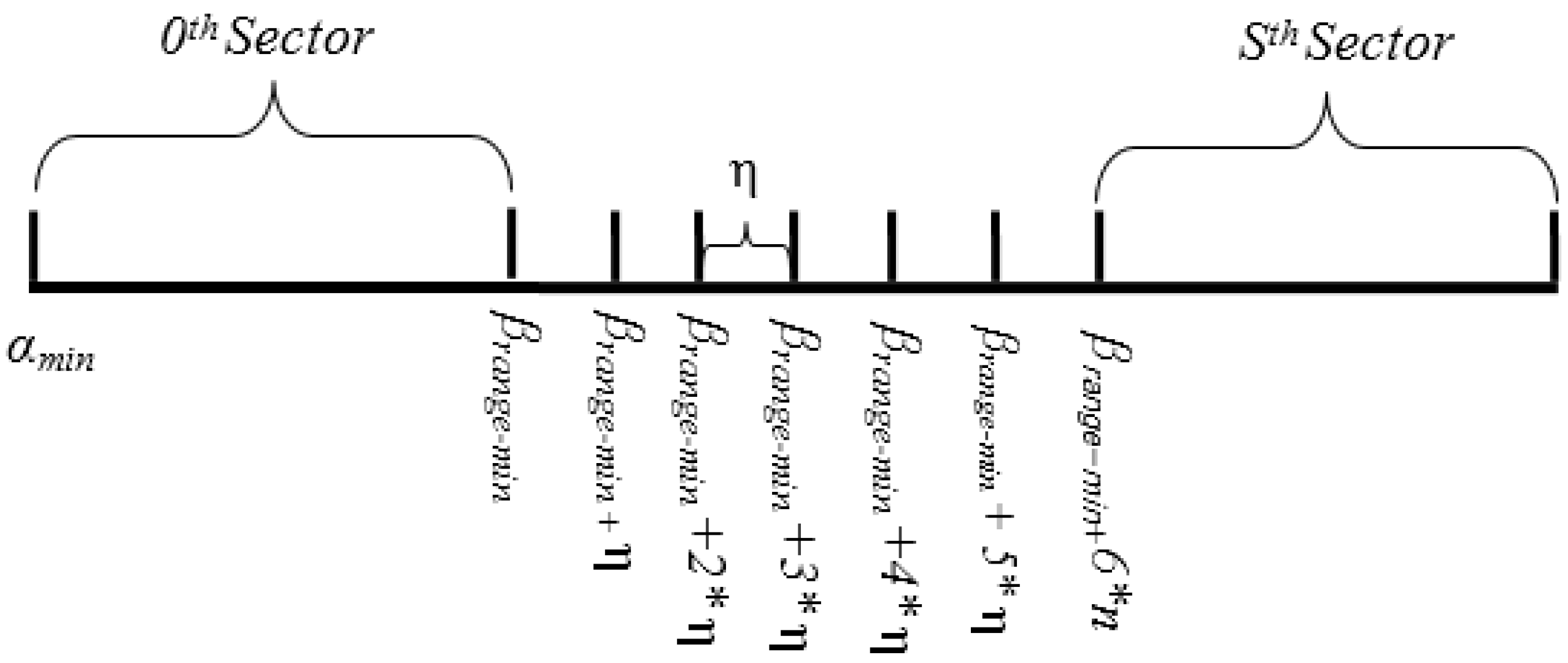
In Equations (7.1)–(7.4), A_i(min), A_i(max), A_i(avg) and A_i(θ) denote the minimum, maximum, average and threshold value of ith attribute. Based on Equations (7.1) and (7.2), the domain of the hash key, denoted by H_D, is α (α_min, α_max). The center of gravity, denoted by β, is derived in Equation (7.3) to find the normalized center point of the domain of the hash key H_D, whereas δ is the separating factor between two pivot points. However, in order to balance the load among sectors, it is important to find the range where the concentration of the data points is high. Hence, β and δ can be used to find the range for center of gravity, denoted by β (β_range-min, β_range-max), as shown in Equation (8).

$$\begin{array}{c}{\beta }_{range-\min }=\beta -\delta \\ {\beta }_{range-\max }=\beta +\delta \end{array}$$

(8)

Thus, the separating step, denoted by η, between two pivot points in COM range can be defined by:

$$\eta =\raisebox{1ex}{$\left({\beta }_{range-\max }-{\beta }_{range-\min }\right)$}\!\left/ \!\raisebox{-1ex}{$S-1$}\right.$$

(9)

Thus, the pivot points for S sectors can be defined in each sector head by:

$${\mathrm{{\rm P}}}_i=\{\begin{array}{l}{\alpha }_{\min },\hfill \\ {\beta }_{range-\min }+i\times \eta ,\hfill \\ {\alpha }_{\max },\hfill \end{array}\begin{array}{c}\\ \\ \end{array}\begin{array}{l}i=0\hfill \\ 0<i<S\hfill \\ i=S\hfill \end{array}$$

(10)

Algorithm 1. Pivot Point Generation Algorithm (implemented at each SH node).

Input:  attrRangeTable (containing minimum, maximum, average and theta of each attribute), W (weights to different attributes based on their importance in the event description).

Output: P (derived pivot point for each sector)

1: mapRec.minRange = mapRec.maxRange = 0

2: m = lengthof (attrRangeTable)

3: for i = 1 to m do

4: mapRec.minRange+=(attrRangeTable[i].min/attrRangeTable[i].max) × W[i]

5: mapRec.maxRange+=(attrRangeTable[i].max)/attrRangeTable[i].max)× W[i]

6: mapRec.com += (attrRangeTable[i].avg)/attrRangeTable[i].max) × W[i]

7: mapRec.theta += (attrRangeTable.theta)/attrRangeTable[i].max) × W[i]

8: i = i + 1

9: end for

10: comLowerLimit = mapRec.com - mapRec.theta

11: comUpperLimit = mapRec.com + mapRec.theta

12: η = (comUpperLimit - comLowerLimit)/(S - 1)

13: for j = 0 to S

14: if (j == 0) then P[j] = mapRec.minRange

15: else if (j == S) then P[j] = mapRec.maxRange

16: else P[j] = comLowerLimit + j × η

17: end if

18: j = j + 1

19: end for

Figure 5. Pivot point generation example.

Figure 5. Pivot point generation example.

Algorithm 1 uses Equations (8)–(10) for calculating pivot points. Figure 5 illustrates the domain and sub-domain of pivot points.

3.3.2. Mapping

Given l attributes in an attribute list associated with weight w_j (1 ≤ j ≤ l) in a WSN application, the source SH_k generates the hash value by:

$$h={\displaystyle \sum _{j=1}^l\left(\left(av{g}_{i=1}^{M_k}{v}_{ij}/A_{j(\max )}\right)\times w_j\right)}$$

(11)

Hence, after each epoch, SH_k forwards the aggregated event $E_k=\langle \left[{\psi }_1,{\psi }_2,\dots ,{\psi }_l\right],\left[t,h\right]\rangle$, where t denotes the epoch number, to the destination sector head denoted by SH_i where, $P_i\le h<P_{i+1}$ and P_i and P_i+1 is the lower and upper limit of ith sub-interval, respectively.

3.4. Insertion

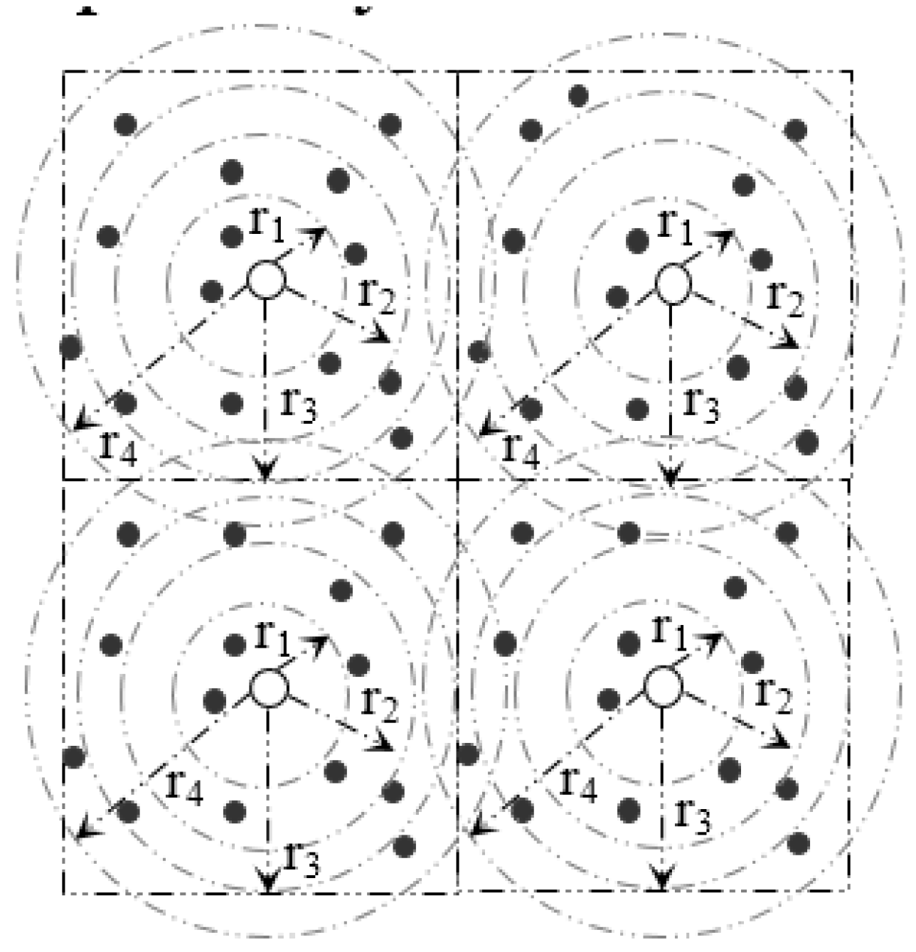
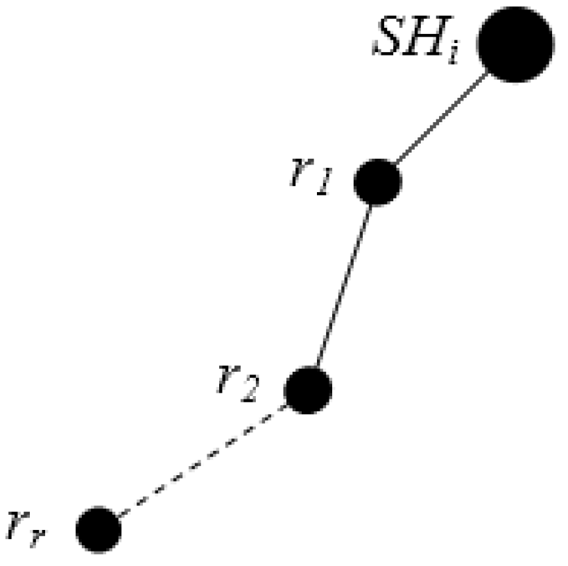
Within a sector, data are further distributed among nodes according to their distance from the SH. In order to do so, a sector is divided into segments. Figure 6 and Figure 7 and Table 2 illustrate the idea of sector segmentation. Given a kth sector containing M_k member nodes, the SH_k first sorts all member nodes based on RSSI in ascending order. The member nodes are then divided into r segments. Each segment forms a circle, denoted by B_(X,Y) (r_i), where the center of the circle is (X, Y) with radius r_i. (X, Y) is the geographic co-ordinates for SH_k. The number of segments depends on the WSN application, sector size and the number of member nodes in each sector. Thus the set of sensors that are within a Euclidean distance r_i from (X, Y) form the segment defined by:

$$B_{(X,Y)}(r_i)=\left\{SensorsCoordinate\left(x,y\right):\left|\left(X,Y\right),\left(x,y\right)\right|\le r_i\right\}$$

(12)

$${\beta }_k=\left({\mathrm{{\rm P}}}_{k+1}-{\mathrm{{\rm P}}}_k\right)/r,\begin{array}{cc}& 1\le k\le S\end{array}$$

(13)

$${\left\{{\mathrm{{\rm P}}}_{M_K(i)}\right\}}_{k=1}^S=\{\begin{array}{l}{\mathrm{{\rm P}}}_k,\hfill \\ {\mathrm{{\rm P}}}_k+\beta \times i,\hfill \\ {\mathrm{{\rm P}}}_{k+1},\hfill \end{array}\begin{array}{l}\hfill \\ \hfill \\ \hfill \end{array}\begin{array}{l}i=0\hfill \\ 0<i<r\hfill \\ i=r\hfill \end{array}$$

(14)

By Equations (13) and (14), the pivot points of r segments within the kth sector are calculated. An event with hash value, denoted by h, is stored in a member sensor node of ith segment where ${\mathrm{{\rm P}}}_{M_K(i)}\le h\le {\mathrm{{\rm P}}}_{M_K(i+1)}$. In order to balance the load, data are distributed among the nodes inside a segment in a round robin fashion (see Algorithm 2).

Algorithm 2. Search_Target_Node (segment[i]), implemented at each SH node.

Input:  segment[i] (a data structure containing member node ID and tally to count the number of packets stored in this member node)

Output: return the target Member Node ID.

1: sort segment[i] in ascending order based on segment[i].tally

2: segment[i].tally = segment[i].tally +1

3: memberNodeId = segment[i].ID

4: return memberNodeId

Figure 6. Formation of Segments inside a Sector.

Figure 6. Formation of Segments inside a Sector.

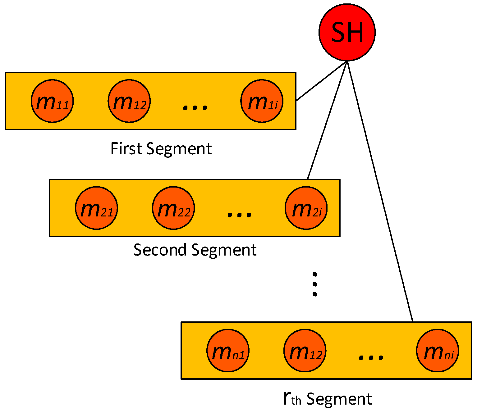
Figure 7. Segmentation architecture of member nodes inside a sector.

Figure 7. Segmentation architecture of member nodes inside a sector.

Table 2. Member table of a SH node.

Table 2. Member table of a SH node.

3.5. Skyline Query

A threshold based hierarchical approach has been used in this research to calculate DS (q, r). The threshold based hierarchical approach uses the temporal correlation among the sectors and segments of a sector. All the key notations used in this section are listed in the Table 3 to increase reader comfort.

Table 3. Skyline Notation.

Symbol	Description
ei	An event at SHi or segment ri of a sector
E	A set of events
θi	The threshold point of SHi or Segment ri
LDSi	The local dynamic skyline of SHi or Segment ri
$e_i{\prec }_{\left(q,r\right)} e_j$	Event ej is dominated by event ei with respect to query point q and the target region of interest is a circle of radius r centered at q.
$e_i{\preccurlyeq }_{\left(q,r\right)} e_j$	Event ej is dominated by or equal to event ei with respect to query point q and the target region of interest is a circle of radius r centered at q.
$e_i{\prec }_{\left(q,r\right)} E$	Each event in E is dominated by event ei with respect to query point q and the target region of interest is a circle of radius r centered at q.
$e_i{\preccurlyeq }_{\left(q,r\right)} E$	Each event in E is dominated by or equal to event ei with respect to query point q and the target region of interest is a circle of radius r centered at q.

Table 3. Skyline Notation.

Symbol	Description
ei	An event at SHi or segment ri of a sector
E	A set of events
θi	The threshold point of SHi or Segment ri
LDSi	The local dynamic skyline of SHi or Segment ri
$e_i{\prec }_{\left(q,r\right)} e_j$	Event ej is dominated by event ei with respect to query point q and the target region of interest is a circle of radius r centered at q.
$e_i{\preccurlyeq }_{\left(q,r\right)} e_j$	Event ej is dominated by or equal to event ei with respect to query point q and the target region of interest is a circle of radius r centered at q.
$e_i{\prec }_{\left(q,r\right)} E$	Each event in E is dominated by event ei with respect to query point q and the target region of interest is a circle of radius r centered at q.
$e_i{\preccurlyeq }_{\left(q,r\right)} E$	Each event in E is dominated by or equal to event ei with respect to query point q and the target region of interest is a circle of radius r centered at q.

Algorithm 3. Build_Tree(), implemented at each SH.

Input:  n (total number of sectors (columns)), SELF_NET_ADDR

Output:  Node (to store the node values), L (to store the address of left child of each node), R (to store the address of right child of each node)

1: // Finding the Track (row) number of current sector

2: i = (SELF_NET_ADDR)/n;

3: index = S;

4: for j = 0 to S−1;

5:   node [j] = (i, j)

6:   if (i-1 ≥ 0)

7:    L[j] = index;

8:    N[index] = (i−1, j)

9:   end if

10:   Li = i−1

11:   while (Li-1≥0)

12:    L[index] = index + 1

13:    Node[index] = (Li−1, j)

14:    index++

15:    Li--;

16:   end while

17:   index++

18:   if (i+1<T)

19:    R[j] = index;

20:    N[index] = (i+1, j)

21:   end if

22:   Ri = i+1

23:   while (Ri+1<T)

24:    R[index] = index+1

25:    N[index] = (Ri+1, j)

26:    index++

27:    Ri++

28:   end while

29:   index++

30: end for

3.5.1. Tree Structure Construction

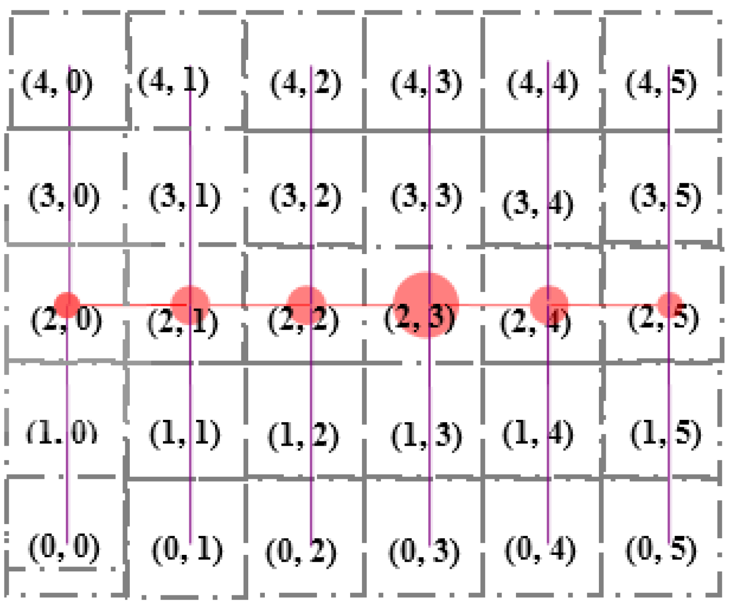
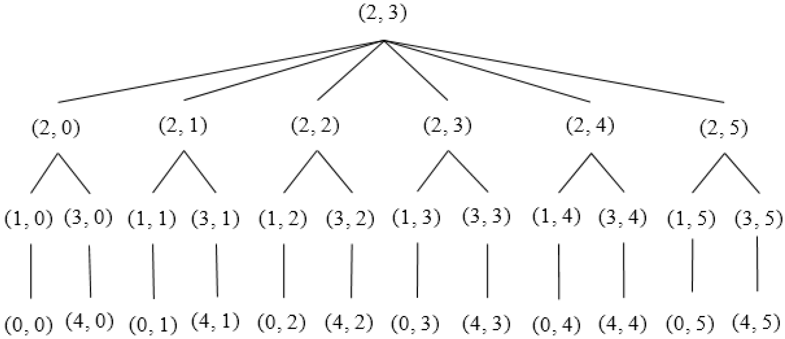
Each SH constructs a tree considering itself as the root using Algorithm 3. Figure 8 and Figure 9 illustrate an example of the formation of a tree rooted at the 13th (2, 3) Sector. Sector (2, 0), (2, 1), (2, 2), (2, 3), (2, 4) and (2, 5) are the child nodes of Sector (2, 3). The sectors lying at the same column but upper row and lower row of each of the child nodes of root node are added to the left and right branch, respectively. For example, Sector (1, 0), (0, 0) and (3, 0), (4, 0) are added to the left and right branch, respectively, of Sector (2, 0). The hierarchy is further maintained among segments inside each sector, as shown in Figure 10.

Figure 8. SH of 13th Sector implies Algorithm 3 in order to convert the 5 × 5 grid into a tree rooted at 13th (2, 3) Sector.

Figure 8. SH of 13th Sector implies Algorithm 3 in order to convert the 5 × 5 grid into a tree rooted at 13th (2, 3) Sector.

Figure 9. Tree rooted at 13th Sector (2, 3).

Figure 9. Tree rooted at 13th Sector (2, 3).

Figure 10. Hierarchy based on segmentation.

Figure 10. Hierarchy based on segmentation.

3.5.2. Basic System Operation

A query node first calculates hash h_q using Equation (10) for the Dynamic Skyline Query (DS (q, r)). The query is then forwarded to the SH_i where P_i ≤ h_q ≤ P_i+1. SH_i finds the range of the query, i.e., [h_q-r, h_q+r]. Hence, the target sectors where the sample dataset of the query need to be considered are SH_j, SH_j+1,…, SH_k, here P_j ≤ h_q-r ≤ P_j+1, P_k ≤ h_q+r ≤ P_k+1 and j ≤ k. The threshold based hierarchical approach includes three phases—Tree Propagation, Regular Update and Triggered Query.

SH_i issues a Triggered Query containing LS_i to SH_j+1, SH_j+2 ..., SH_k. The Triggered Query is issued to ensure fetching all possible events that might be included in the final skyline but was not reported during the Regular Update phase. SH_i sends Triggered Query to each of its child SH_j that satisfies LS_i ⋠ θ_j. Any child node SH_j satisfying LS_i ⪯ θ_j can be discarded since no ineligible event can exist in the final skytline. There cannot exist any event that can be eligible to be included in the final skyline. An internal child node SH_j after receiving Triggered Query LS_p from its parent computes LS_j among LS_p and its non-reported points. SH_j then forwards LS_j to each of its children SH_k that satisfies LS_j ⋠ θ_k and waits for a reply with new points that are not dominated by LS_j. SH_j updates the local skyline after receiving replies from all of its child nodes and finally replies to its parent SH_p with the new skyline event set. In contrast, a leaf node SH_j reports nothing if it reports e_j in the first phase or satisfies LS_i ⪯ θ_j. Otherwise, it reports event e_j.

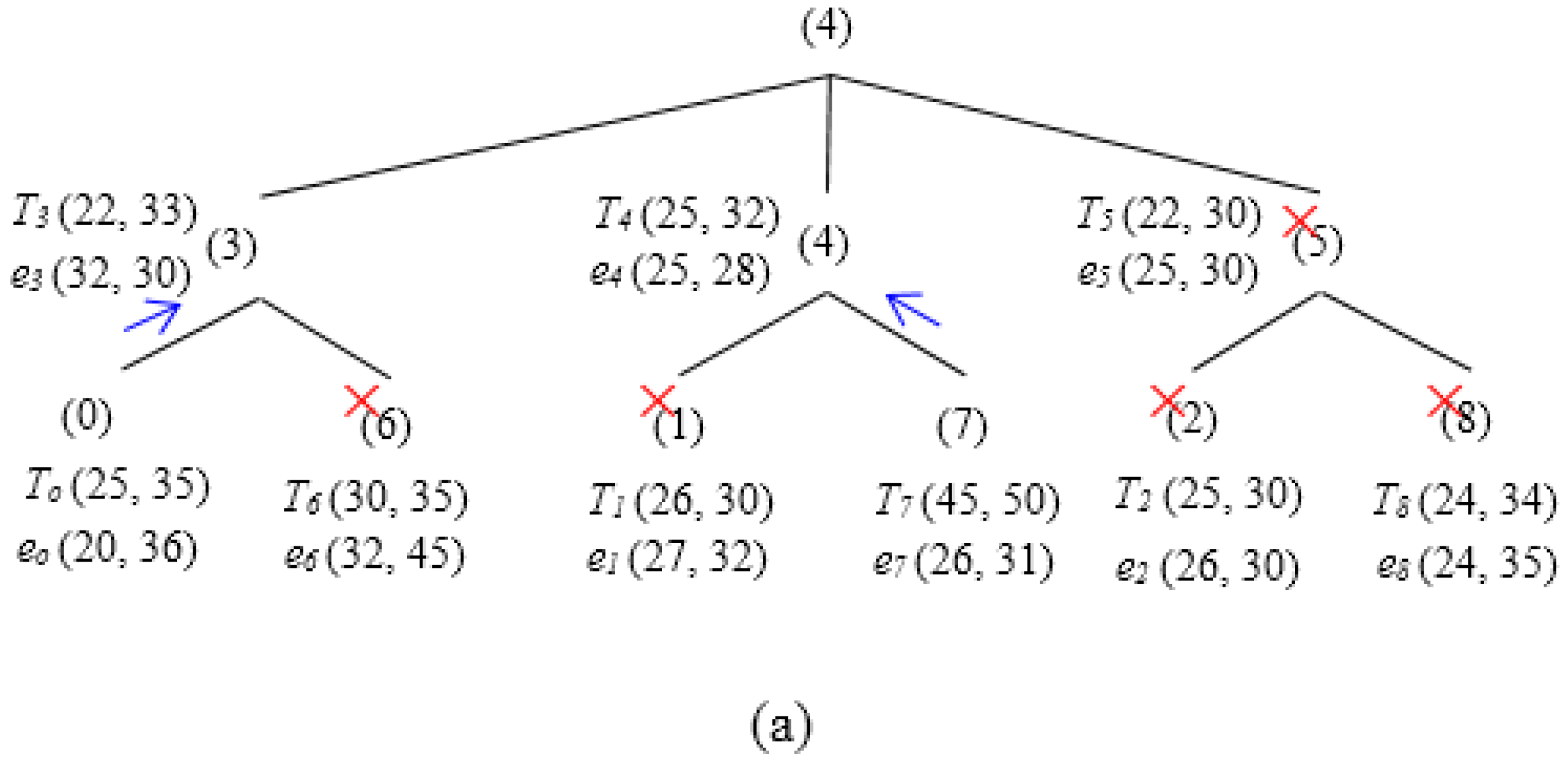
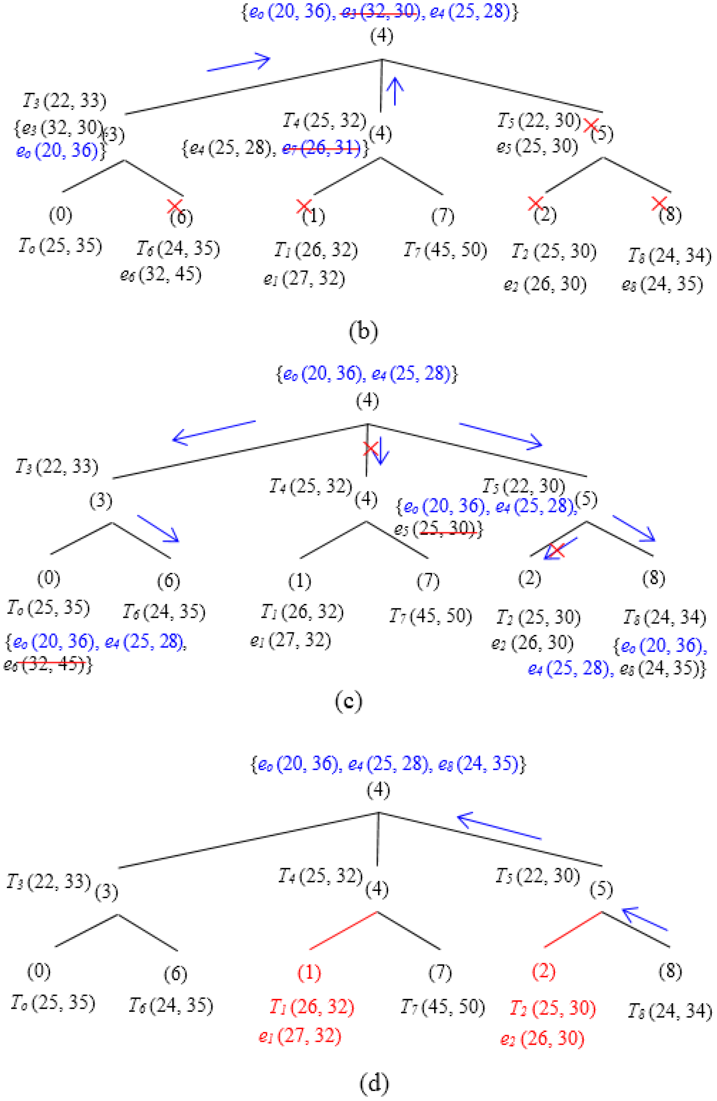
Figure 11 illustrates the functionality of the two phases—Regular Update and Triggered Query in a particular scenario. In the first phase (Regular Update) (Figure 11a), SH₀ and SH₇ reports e_o and e₇ to SH₃ and SH₄, respectively. However, e₇ and e₃ have been pruned by e₄. Thus, the skyline set after the first phase includes {e₀, e₄} (see Figure 11b). Figure 11c,d illustrates the second phase. SH₄ issues a Triggered Query containing {e₀, e₄} to SH₃, SH₆, SH₅, and SH₈ (here, it is assumed that [h_q−r, h_q+r] covers all the tree SH). SH₀, SH₁, SH₇ and SH₂, however, are discarded since their corresponding thresholds are dominated by e₄. After receiving the Triggered Query, SH₅ prunes e₅ and forwards the updated skyline set {e₀, e₄} to SH₈. SH₈ calculates its local skyline and prunes among the query it receives from its parent and its own event e₈. Since e₈ is not dominated, it has also been included into the final local skyline set, i.e., {e₀, e₄, e₈}, and is finally sent back to the SH₄. It is to be noted that, during both phases, SH₁ and SH₂ do not need to transmit any event.

Figure 11. Basic Approach Example (3 × 3 Grids). (a) Regular update. (b) Skyline set after first phase. (c) Triggered query. (d) Skyline set after second phase

Figure 11. Basic Approach Example (3 × 3 Grids). (a) Regular update. (b) Skyline set after first phase. (c) Triggered query. (d) Skyline set after second phase

4. Performance Evaluation

Simulations were conducted using Castalia v3.2 [29] running on top of OMNET++ [31] to evaluate the performance of EDDS. The system parameters and their settings used in the experiments are summarized in Table 4. The network model (illustrated in Section 3.1) was tested in four rectangular fields with different parameter settings. Sensor MAC (SMAC) [32] and Sector Based Distance Routing (SBD) [15] are used in MAC and routing layer. Simulations were run 30~40 times with varying-channel affecting seeds to provide results that included average and 95% confidence interval. In Section 4.1, possible distribution of data throughout the network is presented. Section 4.2 evaluated EDDS in terms of energy consumption, latency and accuracy in a network of 180 nodes in a 90 m × 90 m (8100 m²) rectangular field. In Section 4.3, the performance of EDDS was tested using four different rectangular fields with four different distributions respectively. In Section 4.4, the performance of EDDS is evaluated against SkySensor in terms of data loss, data uniformity, success rate and resilience to node failure.

4.1. Data Distribution

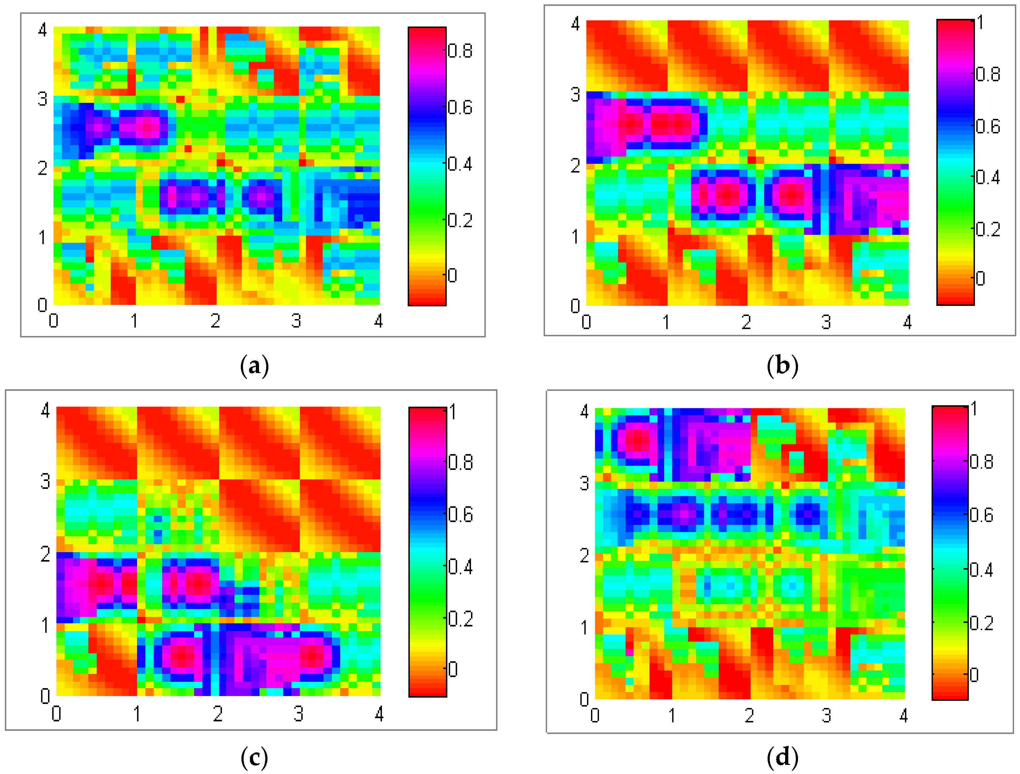
Figure 12 exploits different possible data dispersal with the realization of the mapping algorithm illustrated in Section 3.2. This experiment was conducted in a network of 80 nodes in a 60 m × 60 m (3600 m², total number of sectors is 16 (4 × 4)) field with a 60 min simulation time. The data production rate per sector was five packets per second. Figure 12a shows uniform distribution, which means data are stored uniformly among all sectors of the network. Figure 12b shows a central distribution in which data are usually located among central sector of the network. Figure 12c,d represents the lower bound distribution and upper bound distribution, where data are stored among lower and upper sectors of the network, respectively.

Figure 12. (a) Uniform distribution; (b) central distribution; (c) lower bound distribution; and (d) upper bound distribution.

Figure 12. (a) Uniform distribution; (b) central distribution; (c) lower bound distribution; and (d) upper bound distribution.

4.2. Efficiency

The efficiency of the proposed approach is measured based on three parameters—energy consumption, latency and accuracy. These performance metrics and scalability of the proposed model is directly affected by the query range, which varies based on the average number of sectors indicated by α. 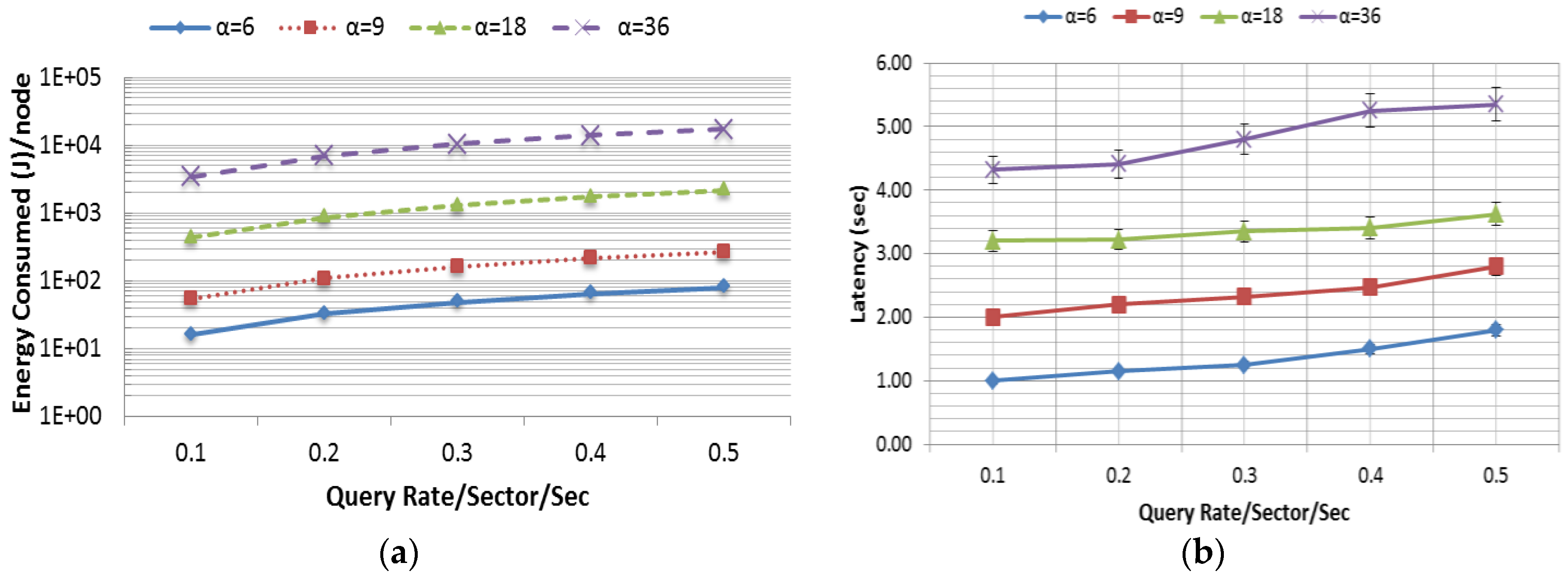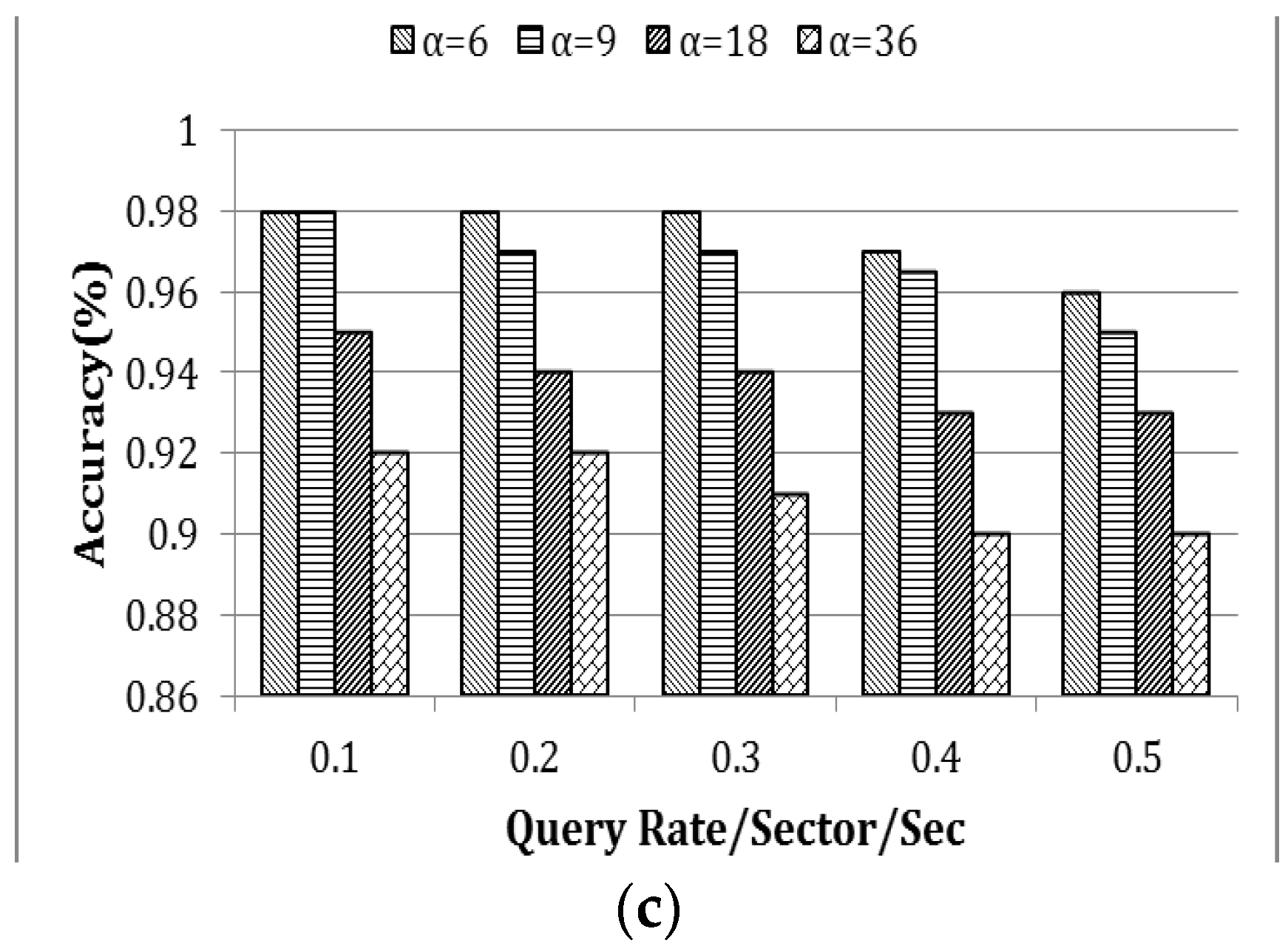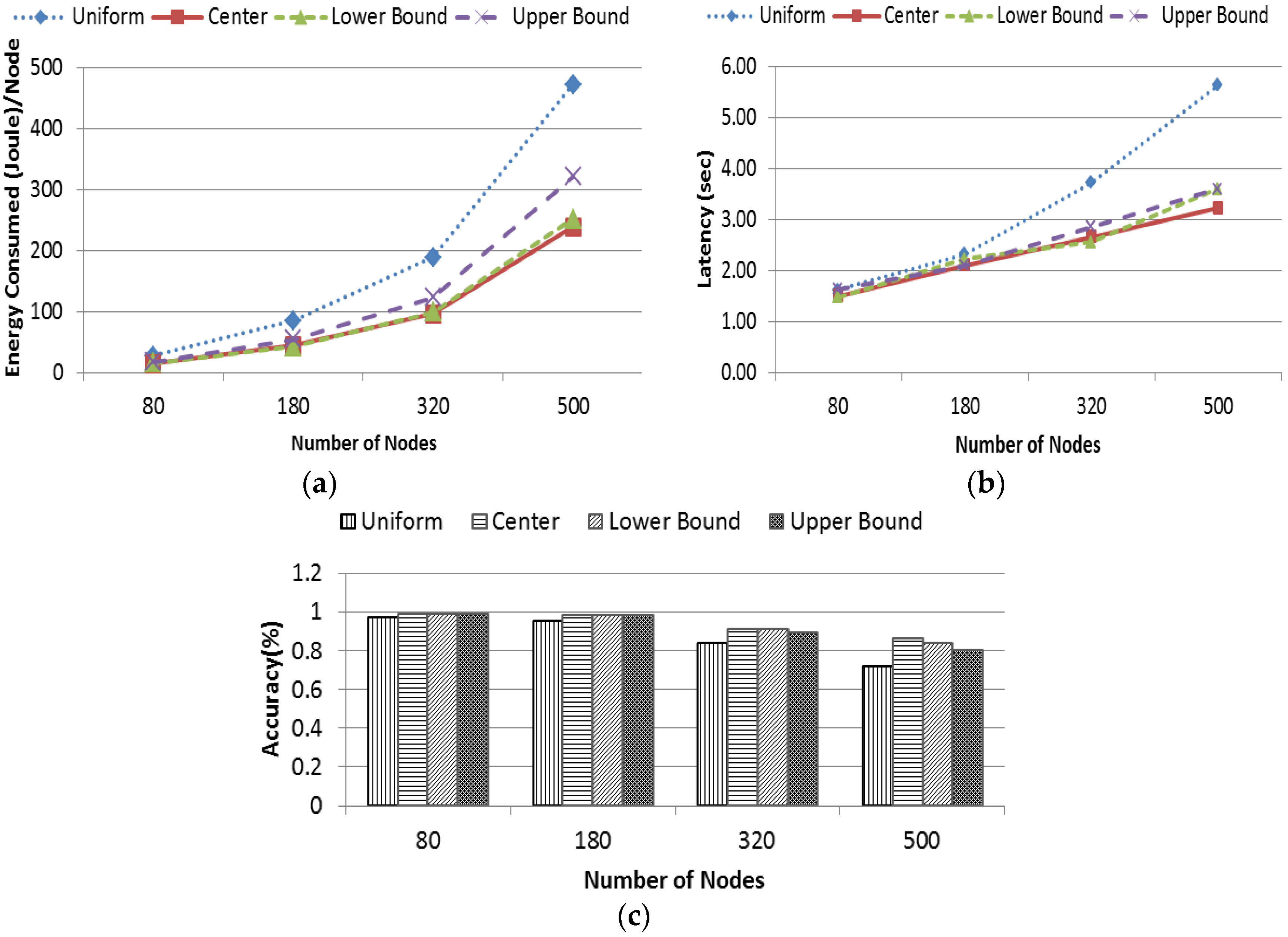With the increase of α, the number of messages that are generated due to three fundamental operations such as Tree Propagation, Regular Update and Triggered Query increases exponentially. Thus, in a model such as skyline query, it is an utmost challenge to minimize the energy consumption and latency while maximizing the accuracy. This experiment was conducted in a 90 m × 90 m rectangular field, in which 180 nodes were randomly and independently disseminated. The data distribution used in this experiment was uniform. The query rate varied from 0.1 to 0.5 queries per sector per second and the simulation was run for 60 min. The Skyline Query overhead is comparatively high due to its three phase query calculation. Figure 13a–c presents the average energy consumption (J) per node, latency (s) and accuracy (accuracy was defined as the percentage of skyline queries that were correctly resolved) as a function of the query rate per sector per second. In this experiment, the query range was varied in four different ways as shown in Figure 13. In order to show the scalability of the system, α has been varied exponentially up to 36, where 36 is the total number of sectors in a 90 m × 90 m (Table 4) rectangular field. From Figure 13a,b, it is noted that the overhead in terms of energy consumption and latency grows radically as α increases. It is also to be noted that the data in Figure 13a are presented in logarithmic scale in order to reduce the wide range to a more manageable size. However, the accuracy of the query response was very high (see Figure 13c) and close to 100%. Packet loss due to interference causes some minor inaccuracy.

Table 4. Simulation Parameters.

Parameter	Setting
Field Size (F)	60 × 60 m2, 90 × 90 m2, 120 × 120 m2, 150 × 150 m2
Number of Nodes (N)	80 (3600 m2), 180 (8100 m2), 320 (14,400 m2), 500 (22,500 m2)
Number of Sectors/Field Size (S/F)	16/(60 × 60 m2), 36/(90 × 90 m2), 64/(120 × 120 m2), 100/(150 × 150 m2)
Member Node Density (fm)	1 node/56.25 m2
Sector Head Node (SH) Density (fSH)	1 node/225 m2
Radio Range (member node)	~8 m
Radio Range (SH)	~20 m
Transmission Power	0 dBm (SH), −5 dBm (member node)
Power Consumption in Sending and Receiving Messages	57.42 mW (SH), 46.2 mW (member node)
Power Consumption Per Sensing	0.02 mJoule
Data Rate, Modulation Type, Bits Per Symbol, Bandwidth, Noise Bandwidth, Noise Floor, Sensitivity	250 Kbps, PSK, 4, 20 MHz, 194 MHz, −100 dBm, −95 dBm
pathLossExponent	2.4
Initial Average Path Loss (PL(d0))	55
Reference Distance (d0)	1.0 m
Gaussian Zero-Mean Random Variable (Xα)	4.0
Routing Protocol	SBD [15]
MAC Protocol, Maximum Transimission Retries	SMAC [32], 2
SMAC Acknowledgment, Synchronization, RTS, CTS Packet Size	11, 11, 13, 13 bytes

Table 4. Simulation Parameters.

Parameter	Setting
Field Size (F)	60 × 60 m2, 90 × 90 m2, 120 × 120 m2, 150 × 150 m2
Number of Nodes (N)	80 (3600 m2), 180 (8100 m2), 320 (14,400 m2), 500 (22,500 m2)
Number of Sectors/Field Size (S/F)	16/(60 × 60 m2), 36/(90 × 90 m2), 64/(120 × 120 m2), 100/(150 × 150 m2)
Member Node Density (fm)	1 node/56.25 m2
Sector Head Node (SH) Density (fSH)	1 node/225 m2
Radio Range (member node)	~8 m
Radio Range (SH)	~20 m
Transmission Power	0 dBm (SH), −5 dBm (member node)
Power Consumption in Sending and Receiving Messages	57.42 mW (SH), 46.2 mW (member node)
Power Consumption Per Sensing	0.02 mJoule
Data Rate, Modulation Type, Bits Per Symbol, Bandwidth, Noise Bandwidth, Noise Floor, Sensitivity	250 Kbps, PSK, 4, 20 MHz, 194 MHz, −100 dBm, −95 dBm
pathLossExponent	2.4
Initial Average Path Loss (PL(d0))	55
Reference Distance (d0)	1.0 m
Gaussian Zero-Mean Random Variable (Xα)	4.0
Routing Protocol	SBD [15]
MAC Protocol, Maximum Transimission Retries	SMAC [32], 2
SMAC Acknowledgment, Synchronization, RTS, CTS Packet Size	11, 11, 13, 13 bytes

Figure 13. (a) Energy consumption; (b) latency; and (c) accuracy.

Figure 13. (a) Energy consumption; (b) latency; and (c) accuracy.

4.3. Robustness

In this section, robustness of EDDS was evaluated through two different experiments with the variation of four different network sizes. In the first experiment, energy consumption, latency, and accuracy were measured for varying the query rate, while, in the second experiment, they were measured for four different data distributions.

4.3.1. Network Size

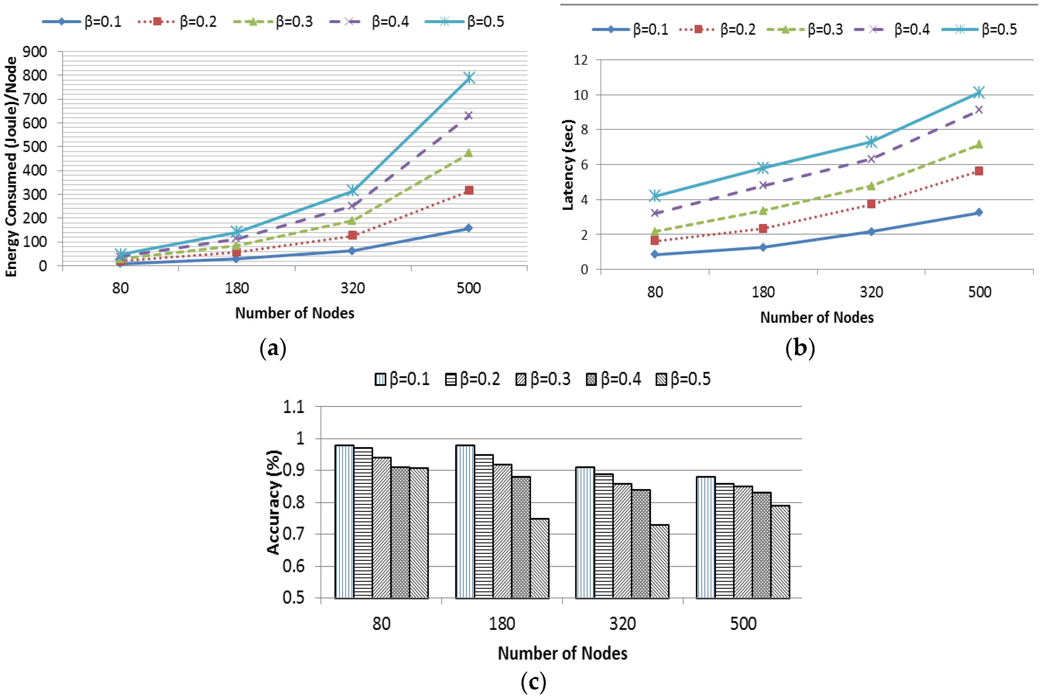
Experiments were carried out by varying the network field sizes such as 60 × 60 m², 90 × 90 m², 120 × 120 m² and 150 × 150 m² containing 80, 180, 320 and 500 nodes, respectively. The size of the region of interest was kept fixed, i.e., the value of α was 9. The rate of the query was varied from 0.1 to 0.5 queries per sector per second. In Figure 14, the rate of the query is represented by β. Figure 14a,b demonstrates that energy consumption and latency is exponentially proportional to the value of β. However, when β is constant, they grow linearly with the size of the network. Figure 14c shows the percentage of accuracy as a function of network size. The accuracy drops slightly with the scale of the network.

Figure 14. (a) Energy consumption; (b) latency; and (c) accuracy.

Figure 14. (a) Energy consumption; (b) latency; and (c) accuracy.

4.3.2. Different Data Distribution

Similarly, Four different data distributions named as uniform, center, lower bound and upper bound distribution (Section 4.1) were considered with the same variation of the network field sizes where the value of α was 9. Figure 15a presents the average energy consumption by each node in different distribution. It is evident that energy consumption in uniform data distribution grows radically. This is because, the data are distributed uniformly through every sector and hence each possible sector (in this case, an average nine neighboring sectors) needed to be scanned to find the target query. The other three distributions had data concentrated in a particular portion of the network. Hence, EDDS required no transmission for the null sector, as they did not store any data. Thus, energy consumption was relatively lower than the uniform distribution. However, center and lower bound distribution have almost similar energy consumption while upper bound distribution falls in the middle. The distribution presented in Figure 12 gives the rational of this behavior. Figure 15b shows the latency performance of EDDS in different distribution. Based on the aforementioned reasoning, it is obvious that the latency in uniform distribution is higher compared to other distribution. Average latency of other three distributions is almost same. Figure 15c shows the accuracy of EDDS in different distributions. It is observed that, accuracy of EDDS drops sharply with the increase of the size of the network. The accuracy of EDDS varies in between 70% and 96% at uniform distribution, 85%–99% at center and lower bound distribution and 80%–99% at upper bound distribution.

Figure 15. (a) Energy consumption; (b) latency; and (c) accuracy.

Figure 15. (a) Energy consumption; (b) latency; and (c) accuracy.

4.4. Evaluation against SkySensor

In this section, EDDS is evaluated against SkySensor in terms of data loss, data uniformity, success rate of the skyline query and resilience to node failure. All subsequent experiments were conducted with a network size of 150 × 150 m² with 500 nodes deployed uniformly. The dimension of attribute varied from 2 to 7, data and query generation rate varied from 0.02 packets/node/second to 0.1 packets/node/second. The default value of data and query rate was 0.02 packets/node/second unless otherwise stated.

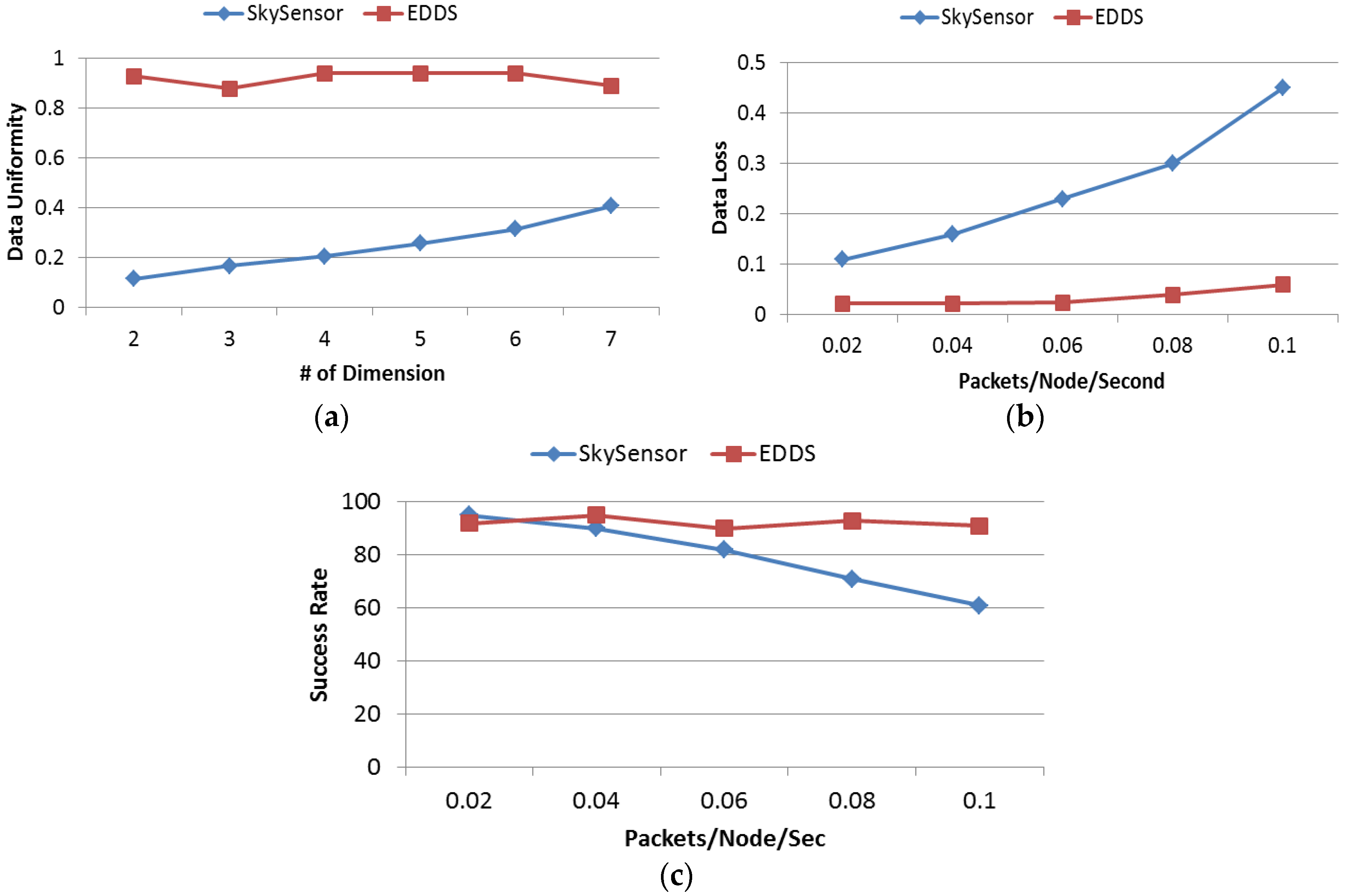
4.4.1. Data Uniformity

In this experiment, data uniformity of SkySensor and EDDS is studied by varying the dimension of attribute from 2 to 7. Uniformity metric is defined as the ratio between the number of nodes used for data storage and total number of nodes in the network. In SkySensor, the number of clusters in a sensor network depends on the number of attributes of a tuple regardless of the size of the network. This is one of the major limitations of SkySensor. On the other hand, referring to Table 4, the number of sectors in EDDS for this particular network is 100, which means data are stored in 100 equivalent clusters of SkySensor resulting uniform distribution of data throughout the network. Figure 16a shows that data uniformity of SkySensor is stringently dependent on the number of dimension while this is independent and consistent for EDDS.

Figure 16. (a) Data uniformity; (b) data loss; and (c) success rate.

Figure 16. (a) Data uniformity; (b) data loss; and (c) success rate.

4.4.2. Data Loss

In this experiment, dimension of attribute was fixed at 2 and data generation rate was varied from 0.02 packets/node/second to 0.1 packets/node/second. Data loss metric is defined as the ratio of the number of data packets actually stored to the total number of packets generated. From Figure 16b, it can be seen that the percentage of data loss in SkySensor increases with an increasing data rate. This happens because there are only two clusters in SkySensor, which is clearly insufficient if the application or simulation runs for a long time. In addition, with a higher data generation rate, a hot spot or bottleneck would be created surrounding the cluster or edge nodes. On the other hand, regardless of the number of dimensions, the number of sectors or clusters is fixed ensuring an increased participation of nodes in data storage with uniform distribution.

4.4.3. Success Rate

Success rate in retrieving a true skyline result is studied by varying the query rate. In this experiment, the number of dimensions in attribute space was fixed at 3. The query rate was varied from 0.02 packets/node/second to 0.1 packets/node/second. Queries were generated uniformly from different parts of the network. From Figure 16c, it is interesting to note that with a low query rate, the success rate of SkySensor is slightly higher than EDDS. However, this result reversed when the query rate was over 0.04 packets/node/second and then the success rate of SkySensor reduced as the query rate increased. This occurred due to the high concentration of all sensor readings around three clusters that eventually created congestion. A significant number of query requests and query responses were lost due to the interference, congestion and hotspot around the edge or gateway of the cluster.

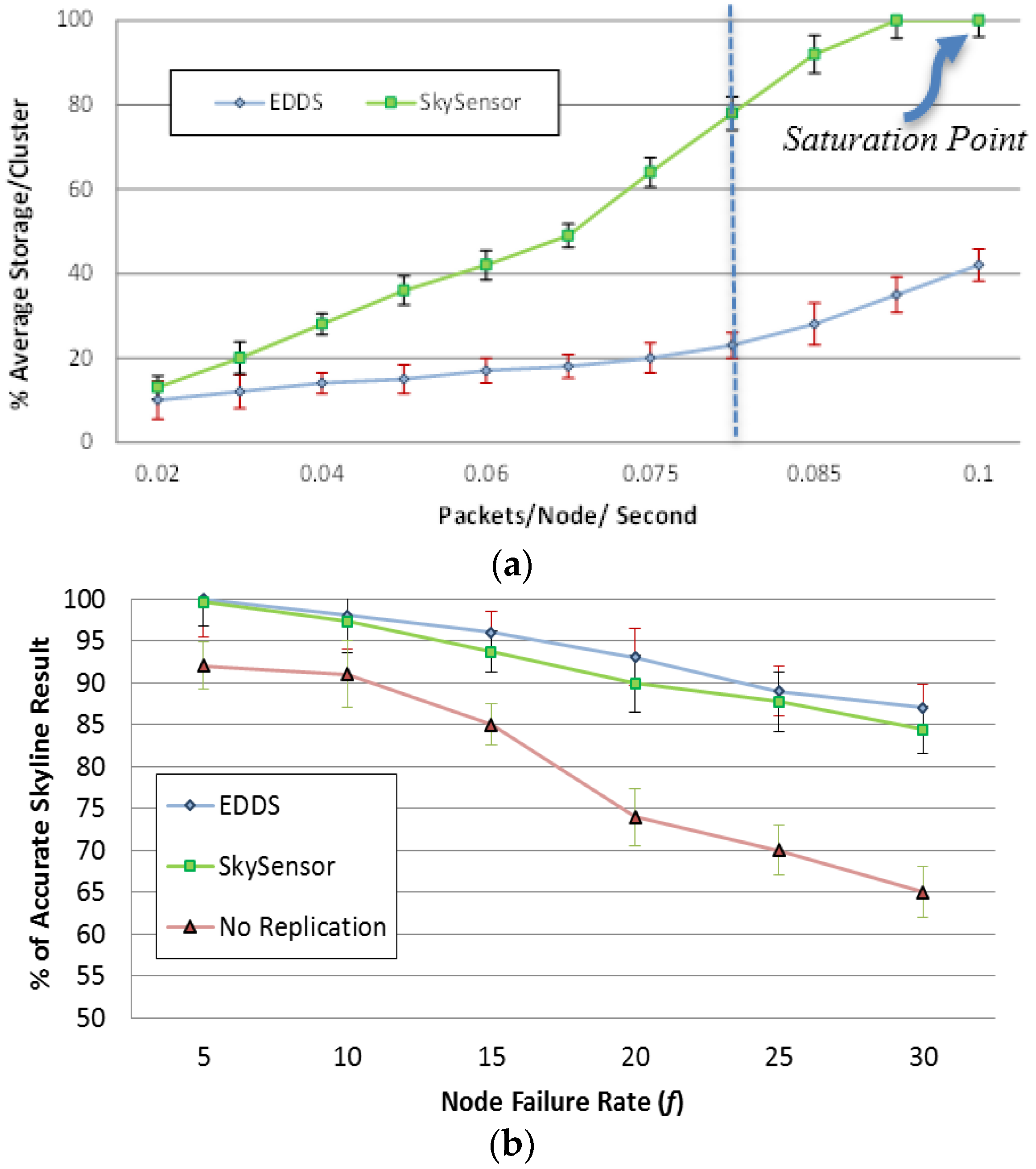
4.4.4. Resilience to Node Failure

In this experiment, the resilience to node failure of EDDS is studied against SkySensor. In SkySensor a local replication method is adopted in order to circumvent data loss due to a storage node failure. On the other hand, EDDS integrates a Decentralized Distributed Erasure Coding (DDEC) algorithm instead of simple replication to achieve similar level of reliability with less redundancy [33]. In this study, the number of dimensions in attribute space was fixed at five and a fraction f of nodes from the network were removed at random point of simulation. The simulation was run for 20 rounds.

In the first sub-experiment (Figure 17a), the data generation rate was varied from 0.02 to 0.1 packets/node/second and f was fixed at 20%. Figure 17a shows that DDEC consumed almost 50% less resources to maintain a similar or even higher magnitude of redundancy in a normal situation (packet rate < 0.08). However, due to the limited number of clusters, the storage space of SkySensor depleted with packet rate greater than 0.08 packets/node/second.

Figure 17. (a) Storage efficiency; (b) Resilience to node failure

Figure 17. (a) Storage efficiency; (b) Resilience to node failure

In the second sub-experiment, data generation rate was fixed at 0.05 packets/node/second and f was varied from 5% to 30%. Figure 17b shows the percentage of the correct skyline result after a query is issued to the network at the end of each round. It is shown that it is possible to get false skyline results. It is shown in Figure 17b that EDDS performance is similar to SkySensor under a lower data production rate. Therefore, EDDS achieves similar or higher level of reliability with less redundancy.

5. Conclusions and Future Work

This paper proposes a distributed approach for resolving DS efficiently in DCS of WSN. To our knowledge, this is the first practical demonstration of DS in DCS of current state-of-the-art WSN. The key feature of EDDS is the dynamic flexibility provided when carrying out queries from distributed data sources. The approach highlights the potential for using distributed skyline queries in the case of DCS of WSN and also shows the relationship between the query efficiency and storage pattern. The experiments provide results for varying WSN configurations and provide detail on the effectiveness of the dynamic skyline query approach. The current research focus is on improving EDDS for large networks and future work includes consideration of reliability and resiliency.