Article

An Experimental Comparison of Radio Transceiver and Transceiver-Free Localization Methods

1
GE Global Research, Schenectady, NY 12309, USA
2
Elect & Computer Engineering, University of Utah, Salt Lake City, UT 84112, USA
3
Xandem Technology LLC, Salt Lake City, UT 84111, USA
*
Author to whom correspondence should be addressed.
J. Sens. Actuator Netw. 2016, 5(3), 13; https://doi.org/10.3390/jsan5030013
Submission received: 17 May 2016 / Revised: 1 August 2016 / Accepted: 8 August 2016 / Published: 17 August 2016
(This article belongs to the Special Issue WSN for Tracking and Localization)

Abstract

:
This paper presents an experimental performance assessment for localization systems using received signal strength (RSS) measurements from a wireless sensor network. In this experimental study, we compare two types of model-based localization methods: transceiver-based localization, which locates objects using RSS from transmitters to receivers at known locations; and transceiver-free localization, which estimates location by using RSS changes on known-location nodes caused by objects. We evaluate their performance using three sets of experiments with different environmental conditions. Our performance analysis shows that transceiver-free localization methods are generally more accurate than transceiver-based localization methods for a wireless sensor network with high node density.

Graphical Abstract

1. Introduction

Localization and tracking of people, robots and assets has significant benefits for logistics, inspection and safety applications. Different sensing techniques such as vision, radio and ultrasound have been developed. Radio-based techniques have the advantages of being robust to different lighting conditions, being able to cover a large area and penetrate non-metal walls, etc. Among all the radio sensing modalities, received signal strength (RSS)-based method provides a low-cost and low-power solution [1], since RSS measurements are available in almost all standard wireless devices. In this paper, we focus on RSS-based localization.
From a wireless sensor network perspective, radio transceivers can be attached to people and objects, and the signal from the known-location receiver nodes of a wireless sensor network can be used to locate and track mobile nodes that are moving or present in the sensor network area. This is the traditional radio transceiver-based method, which uses ranging measurements between transmitters and known-location receivers of a wireless sensor network to locate people wearing those transmitters [2]. The other approach is the transceiver-free or “sensorless sensing” approach [3], which uses characteristic footprint on RSS caused by object motion to detect, locate and track objects. Radio tomographic imaging (RTI) developed by [4] uses the transceiver-free approach, and uses the shadowing losses introduced by objects to RSS links between pairs of nodes in a wireless sensor network to locate these objects. For radio transceiver-based and transceiver-free localization methods, performance analysis has been performed separately, focusing either on transceiver-based or transceiver-free localization. Little effort has been made on comparing the performance of these two RSS-based localization methods in a systematic way. In this paper, we investigate and compare localization accuracy of transceiver and transceiver-free localization methods using experiments specifically designed for both methods.
For transceiver localization, RSS has been used in both fingerprinting-based approach [5,6] and model-based approach [2,7]. However, RSS is a low-cost sensing modality, and it suffers from multipath effects, distorted antenna gain pattern, etc [8]. Thus, a lot of effort has been made on better modeling, algorithms and systems to improve the accuracy and robustness of transceiver-based RSS localization methods [2,5]. In [7], a Cramér-Rao bound (CRB) and maximum likelihood estimator (MLE) were derived under log-normal model for RSS measurements. The MLE location estimation algorithm was implemented in a wireless sensor network, and an extensive RSS measurement campaign illustrated 1 to 2 m root mean squared error (RMSE) using RSS. In a more recent study [9], the non-isotropic antenna gain pattern due to the human body effect was measured and modeled, and an alternating gain and position estimation (AGAPE) algorithm was developed to estimate the orientation and position of a transmitter using RSS measurements at known-location nodes. Their experimental results show submeter level localization and tracking accuracy. In this paper, we focus on model-based transceiver localization and implement the MLE [7] and AGAPE [9] algorithms. We also evaluate their location estimation accuracy using three sets of experiments, and then compare with transceiver-free localization method.
For transceiver-free localization, various methods [10,11,12] have been developed following the “sensorless sensing” approach [3]. Studies in [10,11,13,14] are fingerprinting-based method, which estimates a person’s location by comparing RSS measurements with training measurement database. In this paper, we focus on the other approach, the model-based method, which does not rely on extensive training, i.e., building a “radio map” training database. The model-based transceiver-free localization was initiated by the study in [12], where a spatial elliptical model was developed to characterize the object shadowing effects on RSS links of a wireless sensor network. RTI was then proposed in [4], which images and locates people’s locations based on an empirical model. After that, a variance-based RTI (VRTI) method was developed to locate and track people even through non-metal walls [15]. Since then, different methods have been developed to improve the accuracy and robustness of RTI and VRTI [16,17,18,19,20,21]. In this work, we implement RTI [4], VRTI [15] and subspace variance RTI (SubVRT) [16] algorithms in outdoor, indoor and through-wall scenarios to compare with the performance of transceiver-based localization algorithms.
We organize the paper as follows: Section 2.2 describes transceiver-based localization algorithms including MLE and AGAPE, and Section 2.3 presents transceiver-free algorithms: RTI, VRTI and SubVRT. Section 3 describes datasets collected from three experimental campaigns performed for both transceiver and transceiver-free localization. We present experimental results in Section 4, and we discuss and compare results in Section 4.3.

2. Localization Methods

In this section, we define general terms, and we present transceiver-based and transceiver-free localization methods that we evaluate in this paper. Specifically, we discuss the classical MLE localization algorithm proposed in [7] and the state-of-the-art location and orientation algorithm proposed in [9] for transceiver-based localization. We also formulate model-based transceiver-free localization algorithms RTI [4], variance-based RTI [15], and also the more recent subspace variance radio tomography (SubVRT) [16].

2.1. Problem Statement

For a wireless sensor network with N radio receiver nodes, we use z s , i to denote the coordinate of sensor node i for i { 1 , , N } , and we use z o = [ x o , y o ] T to denote the 2-D coordinate of the object with or without a radio transmitter. For transceiver-based localization, we use s t , i to denote the RSS transmitted from transmitter tag t and measured by node i, and the transceiver-based localization problem is the estimation of the coordinates of the transmitter carried by the object from N RSS measurements s t , i , i { 1 , , N } . Model-based transceiver localization uses the log-distance model to relate RSS measurements with distances, and then estimate transmitter tag location in a trilateration way. Note that even though we focus on formulating localization of a single person here for simplicity, both transceiver and transceiver-free localization methods in this paper are capable of locating multiple persons [22].
For transceiver-free localization, people or objects to be located do not need to carry any radio devices. However, RSS measurements from the wireless links, which the people or objects interact with, need to be collected. We use s f , l to denote the RSS measured at node i l sent by node j l , where i l and j l are the receiver and transmitter number for link l, respectively. We assume L = N ( N - 1 ) directional links measure RSS, and the transceiver-free localization problem is the estimation of z o from L RSS link measurements measured by anchor nodes of a wireless sensor network.

2.2. Transceiver-Based Localization

2.2.1. Model

For transceiver-based localization, a log-distance model [8] is usually used to relate RSS measurements with distances. Here we use a log-distance model with the transmitter antenna gain pattern included in the model [9].
The RSS s t , i measured by node i can be modeled as [9]:
s t , i = P 0 - 10 n p log 10 d i d 0 + g ( α i ) + η
where P 0 is the RSS in dBm at a reference distance d 0 , n p is the pathloss exponent, d i = z s , i - z o is the distance between anchor node i at coordinate z s , i and transmitter t at coordinate z o , α i is the angle between anchor node i and the transmitter, g ( α i ) is the gain pattern in dBi of the transmitter at angle α i , and η is the model error plus noise.
Recent study in [9] shows that the human body changes the gain pattern significantly when the transmitter is worn by a person, and the gain pattern g ( α i ) can be modeled as:
g ^ ( α ) = G 1 cos ( α - β )
where β is the orientation (direction of maximum gain) of the transmitter, and G 1 0 is the magnitude of the cosine function in dB. If G 1 = 0 , we will have a isotropic gain pattern, and Equation (1) converges to the classical log-distance model [8]. Thus, Equation (1) may require more model parameters, but is a more general model that can better characterize the real-world RSS-distance relation.

2.2.2. 2D MLE Algorithm

With an isotropic gain pattern assumption, g ( α i ) = 0 , the maximum likelihood estimation (MLE) is derived by [7] for 2D position estimation:
z ^ o = arg max z o i = 0 N - 1 ( s t , i - μ ( z o ) ) 2
where the RSS values s t , i are assumed to be independent Gaussian with variance σ 2 , and mean μ ( z o ) . Since MLE can be implemented using a 2D grid search method, we also call this method 2D MLE in this paper.
In practice, we first estimate the model parameters n p and P 0 in Equation (1) using linear regression fit of RSS measurements between pairs of anchor nodes. Then we use RSS measurements between the transmitter tag and anchor nodes to estimate the tag location MLE solution.

2.2.3. AGAPE Algorithm

Many previous studies have found the unrealistic isotropic gain pattern assumption [5,23] in RSS-based localization. However, it is the recent study in [9] that first develops models and algorithms to handle, and in fact benefit from, the removal of the isotropic gain pattern assumption.
With a non-isotropic gain pattern as modeled in Equation (2), an alternating gain and position estimation (AGAPE) algorithm [9] is developed to estimate both the position and orientation of a person wearing a transmitter tag in a wireless sensor network.
The basic idea of the AGAPE algorithm is to first use 2D MLE solution Equation (3) as the initial estimate of the transmitter position, and then take advantage of the first-order gain pattern model in Equation (2) to calculate the gain pattern model parameter G 1 and the orientation β:
β = - G ( 1 ) G 1 = 2 N | G ( 1 ) |
where G ( 1 ) is the discrete Fourier transform term G ( k ) = i = 0 N - 1 g ( α i ) e - j α i k with k = 1 .
Given the gain pattern, the log-distance model Equation (1) is used to re-estimate the transmitter position. The algorithm iterates until a misfit function is minimized. The detailed formulation and implementation can be found in [9].

2.3. Transceiver-Free Localization

For model-based transceiver-free localization, the RTI method [4,15,16] uses RSS variations caused by motion or presence of people or object to infer their locations. For single target, the goal of RTI is to estimate an image of the presence of an object in the network space, which can be discretized into P pixels x = [ x 1 , , x P ] T , where x i = 1 if the object occurs in pixel i, and x i = 0 otherwise. The center coordinate of the pixel with the maximum value is the location estimate z ^ o of the object from RTI.

2.3.1. Model

Previous studies [4,12] have shown the efficacy of a linear model to relate the object presence image x with a RSS function denoted by y [4,15]:
y = W x + n
where n is an L-length noise vector, and W is an L × P model matrix with the weight of pixel p on link l formulated as [4]:
W l , p = 1 d i l , j l ϕ if d i l , p + d j l , p < d i l , j l + d w 0 otherwise
where d i l , j l is the Euclidean distance between two sensors i l , j l on link l located at z s , i l and z s , j l ; d j l , p is the Euclidean distance between sensor j l and z p , the center coordinate of pixel p; d i l , p is the Euclidean distance between sensor i l and pixel p; d w is a tunable parameter controlling the ellipse width, and φ is a constant scaling factor.

2.3.2. RTI Algorithms

Once we have the forward model, the localization problem becomes an inverse problem: to estimate P dimensional position vector x from L dimensional link measurement vector y , i.e., the vector of certain RSS function.
We present three RTI algorithms to evaluate and compare with transceiver-based localization: shadowing-based RTI [4], variance-based RTI (VRTI) [15], and subspace variance radio tomography (SubVRT) [16].
Shadowing-based RTI uses the shadowing effect of the human body on correlated RSS link measurements to infer people’s location. The RSS function y used in shadowing-based RTI is the absolute change of RSS with respect to an averaged RSS measured at empty-area calibration period:
y n , l = | s n , l - 1 M i = 0 M - 1 s i , l |
where s n , l n is the RSS at time n for link l, and M is the length of the calibration period. Note that since it is the shadowing-based RTI that first introduced the concept of RTI to the research community, researchers often simply call it RTI, and we also use RTI to represent shadowing-based RTI in this paper.
RTI works well for outdoor environments, but it fails to image people’s location at through-wall situations. Then VRTI is proposed by using the variance of RSS measurements in the RTI framework. It turns out that VRTI is capable of locating human motion even through walls. For VRTI, the RSS function y is the windowed RSS variance:
y n , l = 1 m - 1 i = 0 m - 1 ( s ¯ n , l - s n - i , l ) 2
where s ¯ n , l = 1 m i = 0 m - 1 s n - i , l is the sample average in a time window with length m.
RTI and VRTI have different RSS function y , but they use the same inversion formulation. Their Tikhonov regularized solution is given as:
x ^ = ( W T W + α Q T Q ) - 1 W T y
where α is a regularization parameter, and Q is the Tikhonov matrix, which is calculated by using the difference operations in both the vertical and horizontal directions of an image, as discussed in [15].
VRTI works even through walls, but it is sensitive to all motion including environment intrinsic motion [16]. To make VRTI more robust to environmental noise, a subspace decomposition solution is applied to VRTI, and the SubVRT algorithm is developed. In SubVRT, principal component analysis is used to build an intrinsic subspace and an extrinsic subspace from the covariance matrix of link measurement vector. The SubVRT solution is formulated as:
x ^ = ( W T W + α Q T Q ) - 1 W T ( I - U ^ U ^ T ) y
where U ^ U ^ T is the projection matrix to the intrinsic subspace, and I - U ^ U ^ T is the projection matrix to the extrinsic subspace. Note that, in subspace decomposition, a lower dimensional space spanned by principal components U ^ = [ u 1 , u 2 , , u k ] with the cut-off parameter k represents the space containing the majority of the intrinsic noise, as described in [21].

3. Experiments

3.1. Experiment Campaigns

We use experimental datasets from three experiment campaigns in this paper. In these experiments, we use Memsic TelosB nodes originally developed by UC Berkeley as our radio hardware [24]. We have recorded RSS measurements between a transmitter tag and anchor nodes for transceiver localization, as well as pair-wise RSS measurements between each two anchor nodes for transceiver-free localization. These experiments were performed at outdoor, indoor and through-wall scenarios, which cover a variety of multipath effects and environmental noise conditions:
  • Experiment 1: The first experiment was performed in a 6.4 m by 6.4 m area outside the Merrill Engineering Building of the University of Utah. The area is surrounded by 28 TelosB nodes deployed at known locations near trees and 3 m away from the building wall. A person worn a TelosB node in the middle of his chest and walked around a marked path at a constant speed of about 0.5 m/s. This outdoor experiment dataset was first reported in [9], and details can be found there.
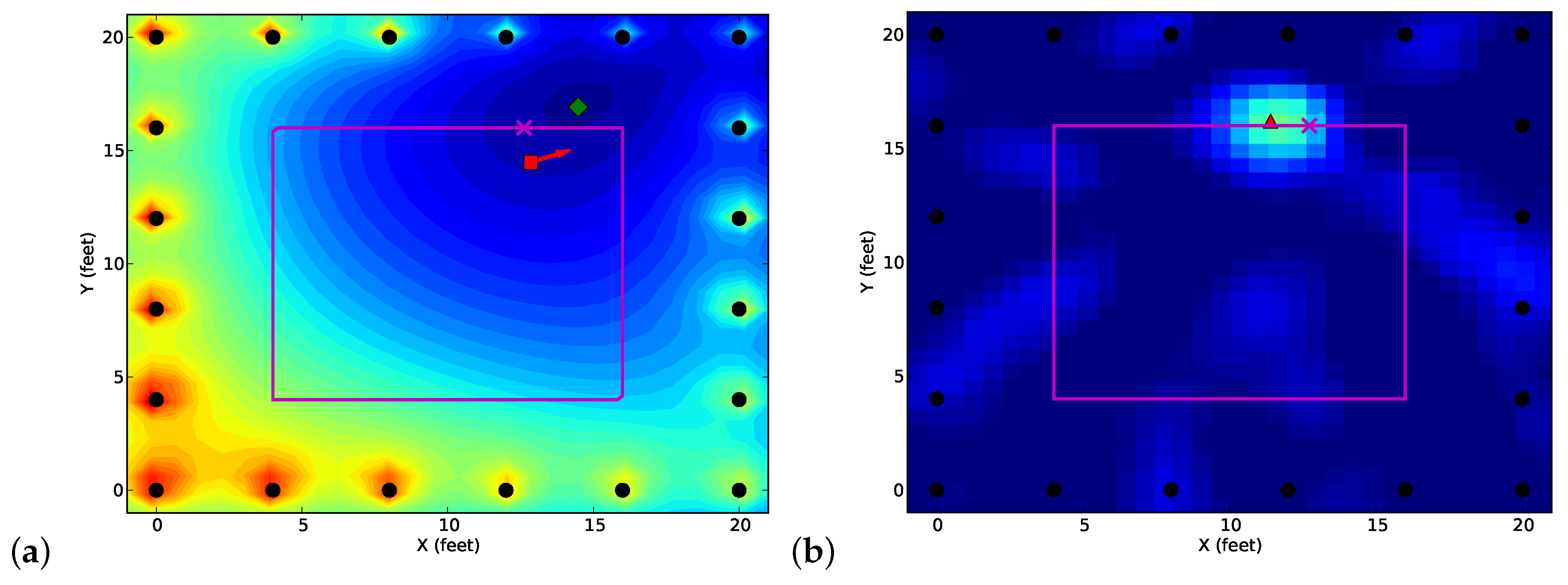
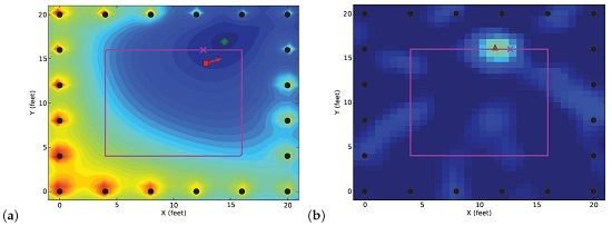
  • Experiment 2: The second experiment was an indoor experiment performed inside the Warnock Engineering Building of the University of Utah. A 6.1 m by 6.1 m area was surrounded by 20 TelosB nodes with an interdistance of 0.91 m (3 feet) between each two anchor nodes. A person wearing a TelosB node walked clockwise twice around a 2.7 m by 2.7 m square, as shown as the purple line in Figure 2. The experiment was performed in the building lounge area, during which students occasionally walked outside the peripheral area of the sensor network. This experiment is first reported by this paper.
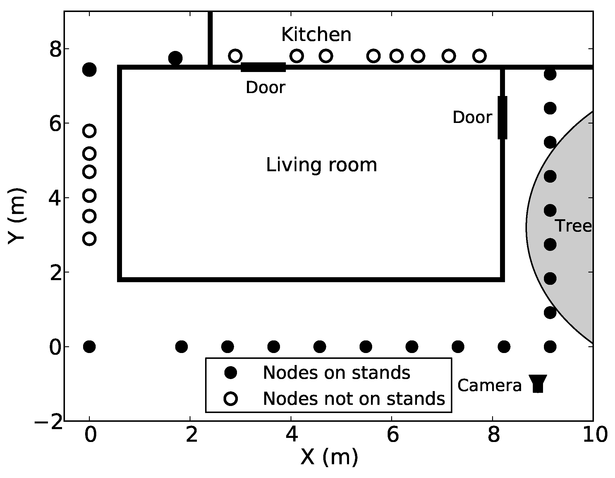
  • Experiment 3: The third experiment was a through-wall experiment, in which 34 TelosB nodes were deployed outside the living room of a residential house, as shown in Figure 1. A person wearing a transmitter walked four times around a 3.6 m by 3.6 m square in the living room. The experiment was performed in a dynamic environment, where wind caused tree branches and leaves to sway and introduced instrinsic noise [21] to the experiment. This experiment was performed by [21], but the transceiver-based experimental dataset is first reported in this paper.

3.2. Network Testbed and Experiment Procedure

All three experiments use the same radio hardware, network protocol and follow the same procedure for transceiver and transceiver-free localization. TelosB nodes were used as network anchor nodes and also mobile node. In all experiments, anchor nodes were deployed at fixed locations, and one mobile node (transmitter tag) was worn by a person in the middle of their chest. All TelosB nodes were programmed with TinyOS program Spin [25], and a basestation connected to a laptop was used to collect pairwise RSS measurements from all these nodes (including the radio transmitter carried by experiment participant). During the experiment, a person wearing the radio transmitter on their chest walked around a marked path a few times. Before people started walking in the area, a calibration was performed with no people in the experimental area. A metronome and a metered path were used to keep the walking speed constant so that the position of the person at any particular time was known. Note that the RSS measurements s t , i recorded by anchor node i for transceiver-based localization, and the RSS measurements s f , l of link l from the network for transceiver-free localization were recorded simultaneously by the network testbed system. Thus, the environmental conditions are the same for the transceiver-based and transceiver-free localization, which ensures a fair comparison between these two localization methods.

4. Experimental Results

4.1. Metrics

We compare the performance of transceiver localization algorithms 2D MLE and AGAPE with transceiver-free localization algorithms RTI, VRTI and SubVRT, in term of accuracy and precision in this section.
To quantify location estimation precision, we use the standard deviation of the estimation error. In addition, we use the root mean squared error (RMSE) of the position estimates, to quantify accuracy:
R M S E = 1 K k = 0 K - 1 ( x k ^ - x o ) 2 + ( y k ^ - y o ) 2
where x k ^ , y k ^ are estimated coordinates at time k, and x o , y o are actual coordinates.

4.2. Results

In this section, we present and compare localization results from transceiver-based methods (2D MLE and AGAPE algorithms) and transceiver-free methods (RTI, VRTI and SubVRT algorithms). We summarize the RMSEs and standard deviations from three sets of experiments in Table 1. We also list path-loss model parameters n p and P 0 showing different environment conditions.

4.2.1. Transceiver Localization Results

For the outdoor Experiment 1, the 2D MLE with an isotropic gain pattern assumption has an RMSE of 2.64 m, as reported by [9]. The large bias is due to the fact that the human body significantly changes the transmitter antenna gain pattern, and the gain pattern has strong directionality. With the addition of a gain pattern model in Equation (2), the AGAPE algorithm is able to achieve an RMSE of 0.87 m.
For indoor Experiment 2 first reported in this paper, we show position estimates from 2D MLE and AGAPE, together with the likelihood function of MLE at a particular time, in Figure 2a. We see the 2D MLE solution corresponds to the maximum of the likelihood function (or the minimum of a cost function), which is biased towards the walking direction of the person, the same as the outdoor Experiment 1. We also see that the AGAPE algorithm estimates both position and orientation of the person. The orientation of the person was facing right at that moment, and the AGAPE estimate has a bias less than 20 . The AGAPE position estimate is better than the 2D MLE estimate. However, AGAPE does not perform as accurate as the outdoor experiment, due to the multipath effect of the indoor environment.
For the through-wall Experiment 3, 2D MLE and AGAPE both have RMSE larger than 2 m. From the histogram of AGAPE estimate errors in Figure 3a, we see that there are several position estimate errors that are larger than 4 m, which is due to the ambiguity problem of AGAPE. That is, AGAPE has the orientation β and gain pattern parameter G 1 to estimate, in addition to position estimate. Thus AGAPE can converge to an incorrect position with an incorrect estimate of orientation, due to the noisy RSS measurements and the modeling error in Equations (1) and (2). We observe this ambiguity problem happened when the person wearing an RFID badge was close to walls. The close proximity of walls could change the transmitter gain pattern, and thus introduce error to the first order gain pattern model. Overall, AGAPE does not have much improvement compared to MLE in Experiment 3.

4.2.2. Transceiver-Free Localization Results

For transceiver-free localization, we run RTI, VRTI and SubVRT on data from Experiments 1 and 2. Since RTI does not work at through-wall environments, we only run VRTI and SubVRT on Experiment 3. For the outdoor Experiment 1, all three algorithms achieve submeter accuracy. RTI has the best performance, an RMSE of 0.41 m. VRTI and SubVRT have slightly higher RMSE, 0.62 m and 0.61 m respectively, since they both need to calculate variance during a time window, and thus their estimates are sometimes lagged behind the true position. Experiment 1 does not have much intrinsic environment noise, thus SubVRT does not have much improvement upon VRTI.
For Experiment 2, one snapshot of RTI image and position estimate is shown in Figure 2b. The image pixel with the maximum pixel value indicates the RTI position estimate. From Table 1, we see that the same as Experiment 1, RTI also has the lowest RMSE 0.33 m, compared to 0.74 m RMSE from VRTI and 0.72 m RMSE from SubVRT. The histogram of RTI estimate errors is shown in Figure 3b. All RTI estimates have error less than 0.8 m.
For Experiment 3, RTI does not work at the through-wall scenario, so we only present VRTI and SubVRT results. Due to the intrinsic environmental noise caused by movement of tree leaves and branches due to wind [16], VRTI has an RMSE of 1.89 m, much larger than those of Experiments 1 and 2. However, SubVRT uses subspace decomposition method to make transceiver-free localization more robust to the intrinsic noise. SubVRT has an RMSE of 0.77 m, 59 % lower than VRTI. Note that in SubVRT, we use k = 10 for Experiments 1 and 2, and k = 40 for Experiment 3, since there is not much intrinsic motion in the first two experiments, while a lot of environment noise exists in Experiment 3, as explained in [16].

4.3. Comparison and Discussion

From the above section, we see AGAPE outperforms 2D MLE in all three experiments, while for transceiver-free localization, RTI has the best performance for Experiments 1 and 2, and SubVRT is the best for Experiment 3. Now we compare transceiver localization algorithm AGAPE with RTI and SubVRT algorithms. For Experiment 1, both the AGAPE algorithm and RTI algorithm achieves submeter localization accuracy. However, the RMSE from RTI is 0.41 m, 52 . 8 % lower than the 0.87 m RMSE from AGAPE. For Experiment 2, the RMSE from RTI is 0.33 m, 80 . 5 % more accurate than AGAPE. The histogram of position errors from RTI and AGAPE are shown in Figure 3a,b, respectively. The RTI errors are all below 0.8 m, and the error standard deviation is 0.14 m. The AGAPE position error has a bimodal histogram, with one mode centered around 1 m, and the other mode of errors larger than 4 m. The large errors of AGAPE are due to the ambiguity problem, in which AGAPE converges to a wrong position with a wrong orientation estimate, due to indoor multipath effect. For the through-wall Experiment 3, the path-loss model parameter n p = 3 . 22 is much larger than those from the first two experiments, due to the attenuation of walls. However, SubVRT still achieves submeter accuracy, an RMSE of 0.77 m, which is over 60 % more accurate than AGAPE and MLE. In sum, the transceiver-free localization algorithms RTI, VRTI and SubVRT outperform transceiver-based localization algorithms MLE and AGAPE in both accuracy and precision, based on three sets of experiments at indoor and outdoor environments.
Comparing the transceiver and transceiver-free localization methods based on three experiments, we reach a counter-intuitive result: RTI-based transceiver-free localization methods are more accurate and precise than transceiver-based methods 2D MLE and AGAPE, even though RTI does not require people to carry any transceivers. However, if we compare the quantities of RSS measurements used in each method, we may understand the reason why RTI achieves better performance. The transceiver-based methods only use the RSS received at the anchor nodes from the transmitter in the localization algorithms. For a network with N anchor nodes, AGAPE and MLE only use N RSS measurements. However, RTI uses all pairwise link measurements from anchor nodes, that is N ( N - 1 ) RSS measurements, if the basestation can reach all nodes in the network. Take Experiment 1 for example, AGAPE achieves 0.87 m RMSE localization accuracy using 28 RSS measurements for each estimate, but RTI uses 756 RSS measurements, which is over an order of magnitude higher than AGAPE. In addition, all three experiments use a wireless sensor network with relatively high node density. The node densities for Experiments 1, 2 and 3 are 0.68, 0.54 and 0.46 node per m 2 , respectively. For a network with low node density, the performance of RTI may be downgraded significantly. We leave this investigation as work to be undertaken in the future.

Author Contributions

Yang Zhao and Neal Patwari conceived and designed the experiments; Yang Zhao performed the experiments and analyzed the data; Neal Patwari contributed materials and analysis tools; Yang Zhao wrote the paper.

Conflicts of Interest

The authors declare no conflict of interest.

References

  1. Mao, G.; Fidan, B.; Anderson, B.D.O. Wireless sensor network localization techniques. Comput. Netw. 2007, 51, 2529–2553. [Google Scholar] [CrossRef]
  2. Patwari, N.; Ash, J.; Kyperountas, S.; Moses, R.M.; Hero, A.O., III; Correal, N.S. Locating the Nodes: Cooperative Localization in Wireless Sensor Networks. IEEE Signal Process. 2005, 22, 54–69. [Google Scholar] [CrossRef]
  3. Woyach, K.; Puccinelli, D.; Haenggi, M. Sensorless Sensing in Wireless Networks: Implementation and Measurements. Second International Workshop on Wireless Network Measurement (WiNMee’06). 2006. Available online: http://www.nd.edu/mhaenggi/pubs/winmee06.pdf (accessed on 13 August 2016).
  4. Wilson, J.; Patwari, N. Radio Tomographic Imaging With Wireless Networks. IEEE Trans. Mob. Comput. 2010, 9, 621–632. [Google Scholar] [CrossRef]
  5. Bahl, P.; Padmanabhan, V.N. RADAR: An in-building RF-based user location and tracking system. In Proceedings of the IEEE INFOCOM 2000, Tel Aviv, Israel, 26–30 March 2000; Volume 2, pp. 775–784.
  6. Roos, T.; Myllymki, P.; Tirri, H.; Misikangas, P.; Sievnen, J. A probabilistic approach to WLAN user location estimation. Int. J. Wirel. Inf. Netw. 2002, 9, 155–164. [Google Scholar] [CrossRef]
  7. Patwari, N.; Hero, A.O., III; Perkins, M.; Correal, N.; O’Dea, R.J. Relative Location Estimation in Wireless Sensor Networks. IEEE Trans. Signal Process. 2003, 51, 2137–2148. [Google Scholar] [CrossRef]
  8. Rappaport, T.S. Wireless Communications: Principles and Practice; Prentice-Hall Inc.: Upper Saddle River, NJ, USA, 1996. [Google Scholar]
  9. Zhao, Y.; Patwari, N.; Agrawal, P.; Rabbat, M. Directed by Directionality: Benefiting from the Gain Pattern of Active RFID Badges. IEEE Trans. Mob. Comput. 2012, 11, 865–877. [Google Scholar] [CrossRef]
  10. Zhang, D.; Ma, J.; Chen, Q.; Ni, L.M. An RF-based system for tracking transceiver-free objects. In Proceedings of the IEEE PerCom’07, White Plains, NY, USA, 19–23 March 2007; pp. 135–144.
  11. Youssef, M.; Mah, M.; Agrawala, A. Challenges: Device-free passive localization for wireless environments. In Proceedings of the MobiCom ’07: ACM Int’l Conf. Mobile Computing and Networking, New York, NY, USA, 9–14 September 2007; pp. 222–229.
  12. Patwari, N.; Agrawal, P. Effects of Correlated Shadowing: Connectivity, Localization, and RF Tomography. In Proceedings of the IEEE/ACM Int’l Conference on Information Processing in Sensor Networks (IPSN’08), St. Louis, Missouri, USA, 22–24 April 2008.
  13. Xu, C.; Firner, B.; Zhang, Y.; Howard, R.; Li, J.; Lin, X. Improving RF-based device-free passive localization in cluttered indoor environments through probabilistic classification methods. In Proceedings of the 2012 ACM/IEEE 11th International Conference on Information Processing in Sensor Networks (IPSN), Beijing, China, 16–19 April 2012; pp. 209–220.
  14. Seifeldin, M.; Saeed, A.; Kosba, A.E.; El-Keyi, A.; Youssef, M. Nuzzer: A Large-Scale Device-Free Passive Localization System for Wireless Environments. IEEE Trans. Mob. Comput. 2013, 12, 1321–1334. [Google Scholar] [CrossRef]
  15. Wilson, J.; Patwari, N. See-Through Walls: Motion Tracking Using Variance-Based Radio Tomography Networks. IEEE Trans. Mob. Comput. 2011, 10, 612–621. [Google Scholar] [CrossRef]
  16. Zhao, Y.; Patwari, N. Noise Reduction for Variance-Based Device-Free Localization and Tracking. In Proceedings of the 8th IEEE Conference on Sensor, Mesh and Ad Hoc Communications and Networks (SECON’11), Salt Lake City, UT, USA, 27–30 June 2011.
  17. Kaltiokallio, O.; Bocca, M.; Patwari, N. Enhancing the accuracy of radio tomographic imaging using channel diversity. In Proceedings of the 2012 IEEE 9th International Conference on Mobile Adhoc and Sensor Systems (MASS), Las Vegas, NV, USA, 8–11 October 2012; pp. 254–262.
  18. Edelstein, A.; Rabbat, M. Background Subtraction for Online Calibration of Baseline RSS in RF Sensing Networks. IEEE Trans. Mob. Comput. 2013, 12, 2386–2398. [Google Scholar] [CrossRef]
  19. Zheng, Y.; Men, A. Through-wall tracking with radio tomography networks using foreground detection. In Proceedings of the 2012 IEEE Wireless Communications and Networking Conference (WCNC), Paris, France, 1–4 April 2012; pp. 3278–3283.
  20. Bocca, M.; Luong, A.; Patwari, N.; Schmid, T. Dial it in: Rotating RF sensors to enhance radio tomography. In Proceedings of the Eleventh Annual IEEE International Conference on Sensing, Communication, and Networking, SECON 2014, Singapore, 30 June–3 July 2014; pp. 600–608.
  21. Zhao, Y.; Patwari, N. Robust Estimators for Variance-Based Device-Free Localization and Tracking. IEEE Trans. Mob. Comput. 2015, 14, 2116–2129. [Google Scholar] [CrossRef]
  22. Bocca, M.; Kaltiokallio, O.; Patwari, N.; Venkatasubramanian, S. Multiple Target Tracking with RF Sensor Networks. IEEE Trans. Mob. Comput. 2013, 13, 1787–1800. [Google Scholar] [CrossRef]
  23. Ladd, A.; Bekris, K.; Marceau, G.; Rudys, A.; Kavraki, L.; Wallach, D. Robotics-based location sensing using wireless ethernet. In Proceedings of the Conference on Mobile Computing and Networking (MOBICOM 2002), Atlanta, GA, USA, 23–28 September 2002; pp. 227–238.
  24. Memsic TelosB Datasheet. Available online: www.memsic.com/userfiles/files/Datasheets/WSN/telosb_datasheet.pdf (accessed on 12 August 2016).
  25. Sensing and Processing Across Networks (SPAN) Lab, Data and Tools Website. Available online: http://span.ece.utah.edu/data-and-tools (accessed on 12 August 2016).
Figure 1. Through-wall experiment (Experiment 3) layout.
Jsan 05 00013 g001
Figure 2. Transceiver and transceiver-free localization results in Experiment 2: (a) Likelihood function for maximum likelihood estimator (MLE) together with MLE and alternating gain and position estimation (AGAPE) estimates; (b) Radio tomographic imaging (RTI) image and estimate (anchor node positions (•); actual person positions (×); AGAPE position estimate (▪); 2D MLE estimate (⧫); AGAPE orientation estimate (⇒)); RTI position estimate (▴).
Jsan 05 00013 g002
Figure 3. (a) Histogram of position estimate errors from AGAPE in Experiment 2; (b) Histogram of position estimate errors from RTI in Experiment 2.
Jsan 05 00013 g003
Table 1. Experimental results from three experiments (unit in meter) 1.
ExperimentModel Parameters2D MLEAGAPERTIVRTISubVRT
n p P 0 RMSEstdRMSEstdRMSEstdRMSEstdRMSEstd
Experiment 11.6748.62.64n/a0.87n/a0.410.120.620.240.610.25
Experiment 22.2819.81.860.781.690.600.330.140.740.330.720.32
Experiment 33.2230.52.100.772.050.78n/an/a1.890.430.770.38
1 : For Experiment 1, we use experimental results reported in [9], which does not contain standard deviation of the position estimate. For Experiment 3, RTI in [4] does not work in the through-wall scenario. We leave those items as n/a.

