Trajectory-Assisted Municipal Agent Mobility: A Sensor-Driven Smart Waste Management System

Abstract

Ubiquity, heterogeneity and dense deployment of sensors have yielded the Internet of Things (IoT) concept, which is an integral component of various smart spaces including smart cities. Applications and services in a smart city ecosystem aim at minimizing the cost and maximizing the quality of living. Among these services, waste management is a unique service that covers both aspects. To this end, in this paper, we propose a WSN-driven system for smart waste management in urban areas. In our proposed framework, the waste bins are equipped with sensors that continuously monitor the waste level and trigger alarms that are wirelessly communicated to a cloud platform to actuate the municipal agents, i.e., waste collection trucks. We formulate an Integer Linear Programming (ILP) model to find the best set of trajectory-truck with the objectives of minimum cost or minimum delay. In order for the trajectory assistance to work in real time, we propose three heuristics, one of which is a greedy one. Through simulations, we show that the ILP formulation can provide a baseline reference to the heuristics, whereas the non-greedy heuristics can significantly outperform the greedy approach regarding cost and delay under moderate waste accumulation scenarios.

1. Introduction

Smart cities operate on the foundation of information and communication technologies in order to bridge citizens and technology with the ultimate goal of improving quality of life and sustainability [1]. Moreover, smart cities manage city assets including, but not limited to, the local departments, information systems, libraries, schools, hospitals, waste management systems and transportation systems [2]. The most commonly-known smart city services are smart transportation, smart grid, smart parking, smart health and smart lighting [3]. Wireless Sensor and Actuator Networks (WSAN) facilitate the manageability and efficiency of smart city services [4,5,6,7]. Most researchers define the smart city paradigm as an application of the Internet of Things (IoT) concept [8]. Besides, the high penetration rate of the IoT technologies, which are used in all the activities of everyday life, is significantly increasing [9].

The Internet of Things (IoT) has been one of the major research topics in the Information and Communication Technology (ICT) field in various applications [9]. Indeed, IoT and WSAN play the key roles in the realization of smart cities, and as stated in [10], a smart city is comprised of water, energy, waste, transportation and information and communication aspects, which are orthogonal to each other. One of the key areas to build sustainable cities is waste management, which stands for acquiring the waste status in the bins through volumetric sensors [11]. Waste accumulation is inevitable in any life cycle [12]. Therefore, waste management is considered to be a factor that directly impacts the quality of living for citizens. Recent research reports that the growth rate of the Municipal Solid Waste (MSW) amount is higher than the urbanization growth rate [13]. In developing countries, the increase of the municipal solid waste generation is correlated with rapid urbanization, an increase in the population and living standards [14]. In the field of waste management, there have been several studies focused on different aspects and challenges [13,14,15,16,17,18,19]. To enable dynamicity in the garbage collection, garbage truck fleet management and determining collection routes, IoT is pointed out as an inseparable component of a waste management system in a smart city infrastructure [20]. To ensure the effectiveness of waste management services, the IoT and WSAN data regarding the waste levels throughout a municipal region call for effective and efficient decision-making systems [21].

In this paper, we propose a WSN-driven smart waste management solution for a smart city setting. To this end, we propose a heuristic method for efficient planning of waste collection routes in the presence of a WSN that raises a set of alarms to initiate/trigger waste collection. We compare the heuristic to a baseline approach, which plans waste management solely based on the next closest location in town. The baseline approach is called Closest Vehicle First (CVF). Two heuristic solutions are developed to improve the naïve approach: (1) Collect based on Upper Threshold (CUT) and (2) Collect based on Upper and Lower Threshold (CULT). The two approaches work similarly; however, CUT keeps adding all the bins to the truck list even if they have not triggered the alarms, whereas CULT aims to collect only the bins with waste levels higher than the lower threshold. Besides, the CUT approach utilizes an upper threshold for the load level of waste bins, whereas the second heuristic takes upper and lower load thresholds into consideration. Through simulations, we show that CUT and CULT improve the baseline solution by up to 16.7% and 8.3% in terms of management cost and by 4.6% and 3% regarding collection delay, respectively. Furthermore, to evaluate the optimality of our heuristic methodology, we formulate an optimization model for the planning of optimal routes for waste collection. Under various small-scale scenarios with different pre-determined sensor-driven alarm thresholds, we show that the proposed heuristic solution can achieve the operation within 85.75% of the solution in real time. The proposed approaches, for the first time, consider the waste arrival rate so as to improve the waste management routing problem. Moreover, considering the waste arrival implicitly gives an indication of the behaviour of filling up the waste bins. Hence, the truck can be directed to collect the bins even if they have not triggered the alarms. Furthermore, the penalty cost considered in the model plays a key role along with the waste arrival rate because overflowed bins are penalized, which would lead to a significant increase in the cost.

This work is organized as follows. In Section 2, we briefly discuss the state of the art in WSN-based waste management in smart cities. Section 3 describes the system model and defines the smart waste management problem. Section 4 provides a thorough explanation of the optimization model for WSN-driven waste management in a smart city setting, while Section 5 presents the baseline approach to address waste management and our proposed heuristic in detail. Section 6 shows numerical results under various test cases by comparing the heuristic to the baseline solution and the optimization model. Finally, Section 7 concludes the article and gives future directions.

2. Related Work and Motivation

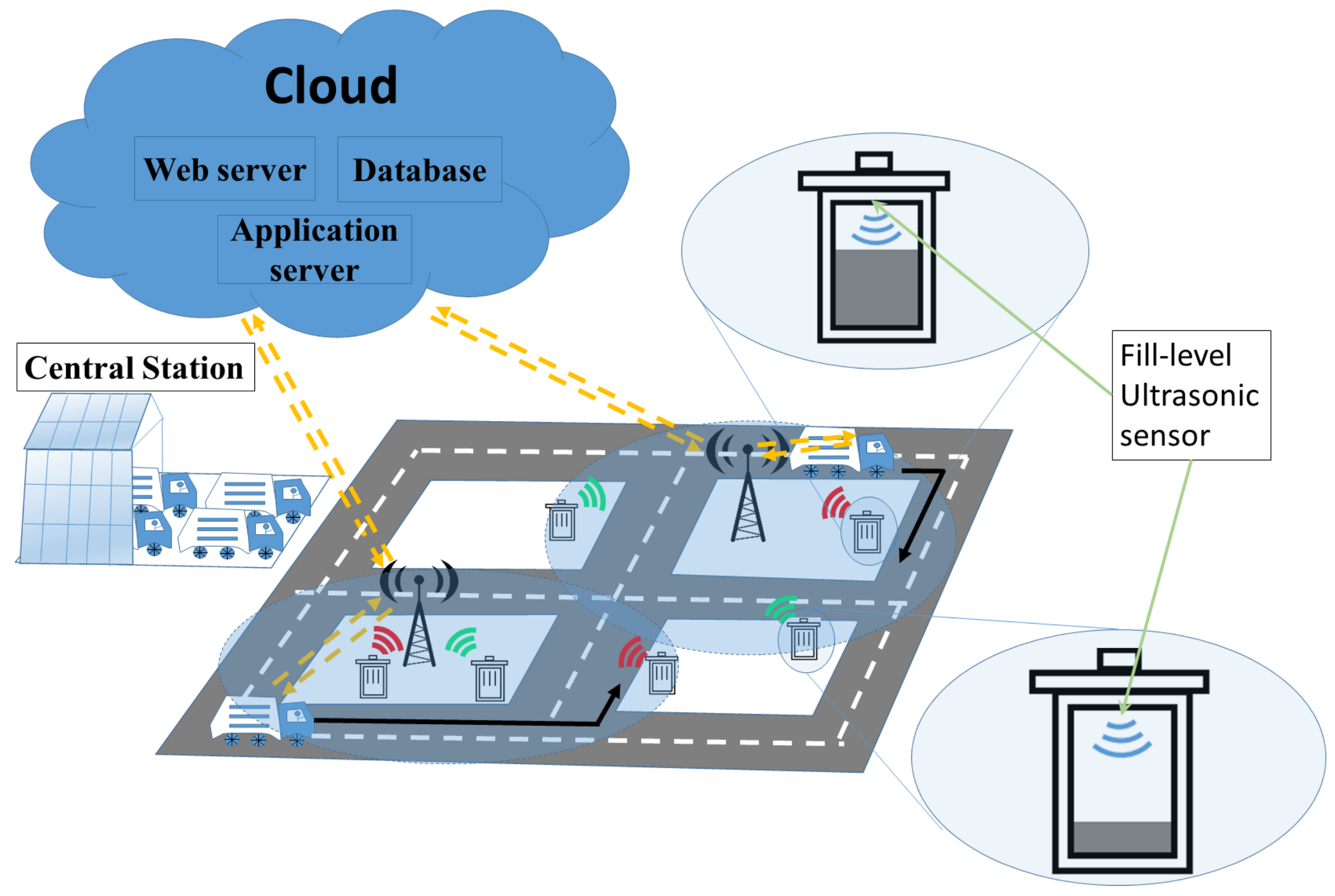
Waste management has been of interest for various researchers in the sustainability and smart cities research field. Urban populations are increasing and causing a change in the consumption patterns. Increasing urbanization speed and scale has caused at least 50% of the global population to reside in urban regions. Moreover, by the year 2050, this ratio is expected to be 86% and 64% of the population for developed and developing countries, respectively [22]. Some studies evaluated different scheduling and routing approaches and their relationships to the fundamental characteristics of the solid waste management system [23]. A comprehensive review of waste management systems for residential units was presented in [24]. Utilization of sensors is particularly considered for monitoring critical parameters such as moisture and temperature instead of the load or residual capacity of waste bins. Such a system can be extended to a city-/municipality-wide monitoring and actuation system through networked sensors and by exploiting the benefits of computational and storage capabilities in the cloud. To this end, we identify the study in [12] as the closest work to ours from the architectural standpoint. In the reference study, a cloud-based waste management system was introduced with the objective of reducing gas/fuel consumption and improving efficiency (i.e., total delay). According to the proposed system, waste bins in a metropolitan area are equipped with sensors that sense and communicate the load levels of the bins to the cloud platform for further processing and decision making. The decision-making module of the proposed system resides in the cloud and provides services for waste collection, route optimization, recycling and disposal, food industry, taxation and even energy generation through waste.

In [20], high priority areas were formed, e.g., schools and hospitals, and priority was given to the bins close to those areas when collecting waste. A dynamic routing process was employed to serve high priority bins immediately. The authors studied four models, namely: (1) the dedicated truck model, (2) detour model, (3) minimum distance model and (4) reassignment model. In the same study, a sector-based approach was formed to partition the area into sectors to which bins and trucks were assigned. However, in some models, trucks can be allowed to serve bins that are located in other sectors. The models listed above were studied under real and synthetic data obtained from the municipality of Saint Petersburg, Russia. The performance of the models was presented with respect to CPU time to form the routes, collected load, distance, routing time, response time and fuel quantity. The results were obtained by varying the number of sectors, prioritizing bins under various scenarios, number of trucks per sector and truck capacity. The study reported that in most cases, the reassignment model outperformed its counterparts regarding the above-mentioned performance metrics. It is worth noting that if a waste management cost function was formulated by incorporating all these metrics, the performance evaluation could be more useful for the overall system.

In [25], the problem of waste management was addressed by planning vehicle routes to collect solid waste in a municipality in Finland. The trucks that collected the bins had capacities that could not be exceeded. In the region under consideration, 30,000 bins were considered to be located in densely- and sparsely-populated districts. Furthermore, different types of municipal solid waste and bins were also considered.

Among the researchers who have contributed to the field of waste management and monitoring, there are exemplary ones who have applied machine learning approaches to their proposals. In [26], level detection for solid waste bins was proposed along with a grey level co-occurrence-based classification.

In [27], the authors aimed to locate an optimal landfill site to achieve minimum economical and socio-environmental effects and cost for the waste management system in the city of Regina (SK, Canada) by integrating Multi-Criteria Decision Analysis (MCDA) with Inexact Mixed Integer Linear Programming (IMILP).

In [28], a real-time framework was developed to monitor the bin status and condition. The monitoring application was based on decision algorithms for sensing solid waste arrival. The route optimization for waste management was envisioned to translate into the minimization of cost and carbon emissions. The authors aimed to minimize the collection cost by performing route optimization in Municipal Solid Waste Collection (MSWC) [29]. The data used in the optimization study was obtained from 39 districts in the city of Trabzon, Turkey. The experiments involve multimedia data that were acquired through video cameras installed in the vehicles. The integration of the Route View Pro${}^T$${}^M$ optimization tool with the Geographic Information System (GIS) enabled finding the shortest route. The proposed approach was shown to reduce the total solid waste collection by 24% via route optimization.

The authors in [30] proposed to utilize bins’ sensors to transmit real-time data of the bins’ fill-level to overcome the uncertainty regarding the amount of waste in the bins. In order to ensure improved efficiency for waste collection, three different operational management approaches were presented: (1) the limited approach, which was based on a cluster first-route heuristic, where the visited bins were selected by their minimum fill-level threshold in each day; after the selection of bins to be collected was defined, a Capacitated Vehicle Routing Problem (CVRP) model was run to optimize each vehicle route in order to achieve minimum transportation cost; (2) the smart collection approach, in which an MILP formulation determined the best collection sequence of bins on each day based on the maximization of the profit; (3) the smarter collection approach, where a heuristic was integrated with the same MILP model to choose the best days that maximized the profit. Out of these approaches, the study concluded that the smart collection was the most efficient and generic one. It is worth noting that the MILP model can also be improved by considering the waste arrival rate and/or a penalty cost that may be applied to the overflowed bins, which can significantly affect the profit.

In [31], Wireless Monitoring Units (WMU) were installed in the waste bins where each WMU was equipped with wireless sensors that monitored the remaining capacity of each bin and reported it to the wireless access points for further processing in a central monitoring station. It was shown that the remaining capacity of a waste bin could be predicted with an accuracy of 98.3%, where a wireless access point could serve a set of WMUs that resided within the coverage of 27 m in diameter.

It is worth noting that data analytics and artificial intelligence methods play a crucial role in profiling the waste arrival, collection and accumulation processes. Therefore, sensory data need to be coupled with data analytics solutions and methodologies. However, this is included in our future agenda. A thorough survey of data analytics approaches for management and profiling of waste management in smart cities was presented in [32].

From the standpoint of the methodology, the study in [30] presented the closest concept to our approach in this article. In the cited work, the authors tackled the problem of obtaining actual load levels in the waste bins through the use of sensors and feeding the information into an optimization model or a sub-optimal heuristic. To this end, three solutions were formulated, where: the first one applied a naive minimum load threshold; the second one aimed to obtain the best collection order of the bins; as an alternative, the authors introduced a further improved model that considered the time dimension, i.e., when and in what order to collect the bins. One of the open issues, as stated by the authors, in their proposed model was the utilization of the waste arrival and accumulation in the bins in the problem. Furthermore, as suggested by the authors, cost factors may vary in time and type. With these in mind, in this article, we incorporate various cost factors into the optimal waste collection model, as well as estimated load levels in the bins.

3. System Model

The waste management problem addressed by our proposed model uses real-time information of the waste fill-levels of the bins to define dynamic routes for each truck. This problem has the following components and inputs: given a complete undirected graph with a set of M waste bins and a distance of ${\Delta }_{ij}$ between any two bins, a central station with a set of N trucks where all the trucks start and end their routes and a disposal area where the trucks dump the waste collected from the bins. Before proceeding with the details of the model, it is worth presenting the notation of the system.

Each waste bin i is defined with a maximum capacity ${\mathsf{\Lambda }}_i$ and is equipped with communication capability to transmit the real-time waste level of the bin measured by an ultrasonic sensor. The sensors inside the waste bins transmit the fill-levels of the bins in m${}^3$s, which is then transformed into kilograms. Furthermore, this particular study is considered for urban areas; thus, it is reasonable to model the waste arrival rate by the Poisson distribution in the cities. Moreover, we present in the Result Section the performance of the system under aggressive arrival rates. However, under significantly light arrival rates, CUT ensures that all the bins on the same assigned route of a truck will be collected regardless of whether or not they have raised an alarm. In the case of an overflow at bin i, a penalty fee of ${\rho }_i$ is applied. Moreover, each truck t has a pre-determined number of workers ($h_t$) and a maximum capacity ($C_t$). All trucks are equipped with two-way communication capability with the base station.

The system model described in Figure 1 shows that all the trucks are initially located in the central station. Once the waste arrival to bin i accumulates and reaches a pre-defined threshold ${\mathsf{\Psi }}_i$, an alarm denoting the call for waste collection is triggered and sent to the base station. The base station communicates with the cloud to process the data and to find the optimal route to collect the waste in loaded bins including the bin that alarmed. The cloud sends the optimal route to truck t through the base station. At the end of the collection, all trucks stop at the disposal area to empty the waste collected from the bins. The objective is to obtain a list of waste bins that are potentially to be visited, and to obtain the optimal visiting trajectory for each truck t, which will minimize the cost value, as well as the collection delay. Referring to the description of the problem, three dynamic waste collection methods are presented in Section 5.

4. Optimization Model for WSN-Based Waste Management in Smart Cities

This section formulates an Integer Linear Programming (ILP) model for the optimal waste management in a smart city in the presence of coordinated wireless sensors for monitoring the waste status at multiple locations. Before we proceed with the details of the optimization, it is worth presenting the notation of the model. The inputs, variables and outputs used in the MILP model are listed and detailed in

Table 1. Basic notations used in the system description. Notations are grouped into three categories: Constants, inputs and variables.

Notations	Equations	Sections	Definition
D	2; 43	4.1; 5.1	Cost of (un)dumping per bin (from a bin to a truck) (€)
H	2; 43	4.1; 5.1	Cost of human resource (€)/h
G	2; 43	4.1; 5.1	Cost of gas mileage (€)/km
S	6; 26; 47	4.1; 4.2; 5.1	Average speed in the town (km/h)
W	2; 26	4.1; 4.2	Time needed to collect waste from a bin (minutes)
N	2	4.1	Total number of trucks
M	2; 13; 36; 43	4.1; 4.2; 5.1	Total number of bins
$UB$	21; 38	4.1; 4.2	The upper bound of variable $P_i$
${\mathsf{\Psi }}_i$	-	5	Upper threshold for the waste amount of bin i
${\psi }_i$	-	5	Lower threshold for the waste amount of bin i
${\rho }_i$	2; 43	4.1; 5.1	Penalty of bin i per kg (€)
$R_t$	6; 26; 47	4.1; 4.2; 5.1	Time needed to empty truck t at the dumping area and prepare it for the next trip (minutes)
ℏ	5; 26; 47	4.1; 4.2; 5.1	Distance from the dumping area to the central station (meters)
${\Delta }_{ij}$	5	4.1	Distance between bin i and bin j (meters)
$t_{ij}$	20; 26	4.1; 4.2	Time needed to move from bin i to bin j (minutes)
${\Delta }_i$	8; 32	4.1; 4.2	Distance from bin i to the dumping area (meters)
$r_i$	7; 33	4.1; 4.2	Distance from the central station to bin i (meters)
${\lambda }_i$	17; 23; 37	4.1; 4.2	Average waste arrival at bin i (kg)
$h_t$	2; 43	4.1; 5.1	Number of workers in truck t
${\mathsf{\Lambda }}_i$	2; 43	4.1; 5.1	Capacity of bin i (kg)
${\delta }_i$	17; 37	4.1; 4.2	Initial load for bin i (kg)
$C_t$	17; 37	4.1; 4.2	Capacity of truck t (kg)
$T_i$	20	4.1	Time from the central station to first bin i (minutes)
$c_t$	-	5	Initial load of truck t (kg)
K	-	5	Threshold for the count of bins that have alarmed
k	-	5	Number of bins that have alarmed
$A_i$	-	5	Alarm status of bin i
B	-	5	List of bins that have alarmed
$Z_t$	-	5	Route of truck t
$L_{ij}$	-	5	List of bins on the shortest path between bin i and j
$Q_{in}^t$	7–21; 27–29; 31–38	4.1; 4.2	The binary variable is one if bin i is the n-th collected bin by truck t
$X_{ij}^{nt}$	5; 9; 10; 11; 16; 26–30	4.1; 4.2	The binary variable defines the multiplication of $Q_{in}^t \mathrm{by} Q_{jn+1}^t$
$H_{in}^t$	17; 18; 19; 37; 38; 39	4.1; 4.2	The integer variable defines the multiplication of $P_i$ by $Q_{in}^t$
$V_{jn}^t$	20; 21; 22; 23	4.1	The integer variable defines the multiplication of $P_i$ by $Q_{jn-1}^t$
$d_t$	2; 3; 5; 6; 44	4.1; 5.1	The integer variable defines the total distance covered by truck t (meters)
d	2; 3; 43; 44	4.1; 5.1	The integer variable defines the total distance covered by Ntrucks (meters)
$I_t$	2; 47	4.1; 4.2; 5.1	The integer variable defines the distance from the central station to first bin of truck t (meters)
$\widehat{I_t}$	2; 47	4.1; 4.2; 5.1	The integer variable defines the distance from last bin of truck t to the dumping area (meters)
${\tau }_t$	4; 6	4.1	The integer variable defines the total time of truck t (minutes)
$\tau$	2; 4; 43; 45	4.1; 5.1	The integer variable defines the total time of the Ntrucks (minutes)
$b_t$	15; 16; 30; 34; 45	4.1; 4.2; 5.1	The integer variable defines the total number of bins collected by truck t
$F_i$	2; 23; 43	4.1; 5.1	The integer variable defines the final load of bin i (kg)
$P_i$	18; 20; 21; 23; 38–41	4.1; 4.2	The integer variable defines the pick up time of bin i (minutes)
$Y_t$	-	5	List of visited bins by truck t

.

4.1. Cost-Based Optimization Model

The objective of the cost-based optimization model is to minimize the cost of waste collection. The objective function in Equation (1) is broken down into the cost components in the set of constraints starting Equation (2). The following parameters contribute to the cost of waste collection: gas mileage, human resource and penalty due to excessively-loaded bins.

$$MinimizeCost$$

(1)

subject to

$$Cost-G·d-\tau ·H·h_t-\sum _{i=1}^M(F_i-{\mathsf{\Lambda }}_i)·{\rho }_i=H·W·M·N·h_t+D·M$$

(2)

$$d-\sum _{t=1}^N{d}_t=0$$

(3)

$$\tau -\sum _{t=1}^N{\tau }_t=0$$

(4)

$$d_t-\sum _{n=1}^M\sum _i^M\sum _{j\ne i}^M{\Delta }_{ij}{X}_{ij}^{nt}=\widehat{I_t}+I_t+\hslash ,\forall t\in N$$

(5)

$${\tau }_t-d_t/S=R_t,\forall t\in N$$

(6)

$$I_t-\sum _{i=1}^M{Q}_{i1}^t·r_i=0,\forall t\in N$$

(7)

$$\widehat{I_t}-\sum _{n=1}^M\sum _{i=1}^M(Q_{i+1,n+1}^t-Q_{in}^t)·{\Delta }_i=0,\forall t\in N$$

(8)

Equations (3)–(8) formulate the distance-related constraints. Equations (3) and (4) define the total distance and total collection time (i.e., route length), respectively. In addition, Equations (5) and (6) define the distance and time covered by each truck. The next constraint in Equation (7) represents the distance from the central station to the first bin. Finally, the constraint in Equation (8) formulates the distance from the last bin to the disposal area.

$$X_{ij}^{nt}-Q_{in}^t\le 0,\forall j\in M,\forall n\in M,\forall t\in N$$

(9)

$$X_{ij}^{nt}-Q_{jn+1}^t\le 0,\forall j\in M,\forall n\in M,\forall t\in N$$

(10)

$$Q_{in}^t+Q_{jn+1}^t-X_{ij}^{nt}\le 1,\forall j\in M,\forall n\in M,\forall t\in N$$

(11)

The optimization model requires formulating the conditional variable that denotes whether bins i and j are picked up by truck t at the n-th and $(n+1)$-th order, respectively. This can be formulated as the multiplication of the two variables, i.e., ($Q_{in}^t\times Q_{in+1}^t$). The non-linearity in $Q_{in}^t\times Q_{jn+1}^t$ is linearized by the constraints in (9)–(11). The first two inequalities ensure that $X_{ij}^{nt}$ will be zero if either $Q_{in}^t$ or $Q_{in+1}^t$ is zero. The last inequality ensures that $X_{ij}^{nt}$ will be equal to one, only if both binary variables are one. However, this will linearize $X_{ij}^{nt}$ without violating any of the other constraints.

$$\sum _{n=1}^M\sum _{t=1}^N{Q}_{in}^t=1,\forall i\in M$$

(12)

$$\sum _{n=1}^M\sum _{i=1}^M\sum _{t=1}^N{Q}_{in}^t=M$$

(13)

$$\sum _{i=1}^M{Q}_{in}^t\le 1,\forall n\in M,\forall t\in N$$

(14)

$$\sum _{n=1}^M\sum _{i=1}^M{Q}_{in}^t-b_t=0,\forall t\in N$$

(15)

$$\sum _{n=1}^M\sum _{i=1}^M{X}_{ij}^{nt}=b_t-1,\forall t\in N$$

(16)

$$\sum _{n=1}^M\sum _{i=1}^M(Q_{in}^t·{\delta }_i+{\lambda }_i·H_{in}^t)\le C_t,\forall t\in N$$

(17)

$$P_i-(1-Q_{in}^t)·UB\le H_{in}^t,\forall i\in M,\forall n\in M,\forall t\in N$$

(18)

$$H_{in}^t\ge 0,\forall i\in M,\forall n\in M,\forall t\in N$$

(19)

The next set of equations denotes the capacity constraints: Equation (12) ensures that bin i can be collected only by one truck. Equation (13) guarantees that all bins must be collected; and the constraint in Equation (14) ensures the following: given truck t, order n can be set to bin i at most once. The constraint set in Equations (12)–(14) ensures that all bins can be visited only once in consecutive order.

The constraint in Equation (15) defines the number of collected bins by each truck, whereas the constraint (16) defines the number of trips made between two consecutive bins. The constraint in Equation (17) ensures that the total bins collected by truck t will not exceed the truck capacity. Similar to the constraints above, the product of the binary variable $Q_{in}^t$ with the integer variable $P_i$ (pickup time of bin i) is linearized where $H_{in}^t$ denotes the product, i.e., $H_{in}^t=Q_{in}^t\times P_i$. Equation (18) ensures that $H_{in}^t$ will have the same value as $P_i$ if $Q_{in}^t$ is one, and zero otherwise. Equation (19) ensures that $H_{in}^t$ will have a non-negative value. Similarly, Equations (21) and (22) solve the non-linearity in Equation (20) the same as the way Equations (18) and (19) do.

Equation (20) formulates the pickup time of bin i by summing the time distance between bins i and j (i.e., $t_{ij}$), pickup time of the previous bin $P_j$ and the time needed to reach the first bin from the central station. Equation (23) defines the final load of bin i by adding the current load (i.e., the multiplication of the pickup time and arrival rate) of the bin to the initial load.

$$P_i-\sum _{j\ne i}^M(X_{ij}^{nt}·t_{ij})-\sum _{j\ne i}^M{V}_{jn}^t-(Q_{i1}^t·T_i)=0,\forall t\in N,\forall i\in M,\forall n\in M,n>1$$

(20)

$$P_i-(1-Q_{in-1}^t)·UB\le V_{jn}^t,\forall i\in M,\forall n\in M,\forall t\in N$$

(21)

$$V_{jn}^t\ge 0,\forall i\in M,\forall n\in M,\forall t\in N$$

(22)

$$F_i-(P_i·{\lambda }_i)={\delta }_i,\forall i\in M$$

(23)

4.2. Delay-Based Optimization Model

In the delay-based ILP model, the constraints in Equations (27)–(42) share the same functionality as the cost model constraints. However, Equation (26) defines the objective function to minimize the truck delay based on the travel time between two consecutive bins, travel time from the central station to the first bin, travel time from the last bin to the dumping area, travel time from the dumping area to the central station, the time needed to empty the bins and time required to unload the truck in the dumping area.

$$MinimizeDelay$$

(24)

subject to

$$Delay-\sum _{t=1}^{N}Dela{y}_t=0$$

(25)

$$Dela{y}_t-\sum _{n=1}^M\sum _i^M\sum _{j\ne i}^M{t}_{ij}{X}_{ij}^{nt}-b_{t}W=(I_t+\widehat{I_t}+\hslash )/S+R_t,\forall t\in N$$

(26)

$$X_{ij}^{nt}\le Q_{in}^t,\forall i\in M,\forall j\in M,\forall n\in M,\forall t\in N$$

(27)

$$X_{ij}^{nt}\le Q_{jn+1}^t,\forall iM,\forall j\in M,\forall n\in M,\forall t\in N$$

(28)

$$Q_{in}^t+Q_{jn+1}^t-X_{ij}^{nt}\le 1,\forall i\in M,\forall j\in M,\forall n\in M,\forall t\in N$$

(29)

$$\sum _{n=1}^M\sum _{i=1}^M{X}_{ij}^{nt}=b_t-1,\forall t\in N$$

(30)

$$\sum _{n=1}^M\sum _{t=1}^N{Q}_{in}^t=1,\forall i\in M$$

(31)

$$\widehat{I_t}=\sum _{n=1}^M\sum _{i=1}^M(Q_{i+1,n+1}^t-Q_{in}^t)·{\Delta }_i,\forall t\in N$$

(32)

$$I_t=\sum _{i=1}^M{Q}_{i1}^t·r_i,\forall t\in N$$

(33)

$$\sum _{n=1}^M\sum _{i=1}^M{Q}_{in}^t=b_t,\forall t\in N$$

(34)

$$\sum _{i=1}^M{Q}_{in}^t\le 1,\forall n\in M,\forall t\in N$$

(35)

$$\sum _{n=1}^M\sum _{i=1}^M\sum _{t=1}^N{Q}_{in}^t=M$$

(36)

$$\sum _{n=1}^M\sum _{i=1}^M(Q_{in}^t·{\delta }_i+{\lambda }_i·H_{in}^t)\le C_t,\forall t\in N$$

(37)

$$P_i-UB(1-Q_{in}^t)\le H_{in}^t,\forall i\in M,\forall n\in M,\forall t\in N$$

(38)

$$H_{in}^t\ge 0,\forall i\in M,\forall n\in M,\forall t\in N$$

(39)

$$P_i-\sum _{j\ne i}^M(X_{ij}^{nt}·t_{ij})-\sum _{j\ne i}^M{V}_{jn}^t-(Q_{i1}^t·T_i)=0,\forall t\in N,\forall i\in M,\forall n\in M,n>1$$

(40)

$$P_i-(1-Q_{in-1}^t)·UB\le V_{jn}^t,\forall i\in M,\forall n\in M,\forall t\in N$$

(41)

$$V_{jn}^t\ge 0,\forall i\in M,\forall n\in M,\forall t\in N$$

(42)

5. Heuristics for WSN-Based Waste Management in Smart Cities

This section describes three heuristic solutions addressing the efficient waste management problem, namely: (1) Closest Vehicle First (CVF), (2) Collect based on Upper Threshold (CUT) and (3) Collect based on Upper and Lower Threshold (CULT). The notations for the constants and inputs presented in Table 1 are also used while describing the heuristics.

5.1. Closest Vehicle First: A Locality-Based Baseline Solution

The CVF model is constructed to address the problem of the waste management by providing an efficient route for the given set of bins that reached their thresholds and raised alarms. In this approach, bins are visited if and only if they raised alarms, so as to reduce the cost by not visiting unnecessary bins that contain an insignificant amount of waste.

The CVF model works as follows: Trucks remain in ready mode to pick up bins until an alarm is raised. Bin i triggers the alarm when the waste level reaches the upper threshold ${\mathsf{\Psi }}_i$. When the number of raised alarms reaches K, the cloud constructs a route (B) between the triggered bins and sends it to a truck t through the base station. The route construction is based on Dijkstra’s shortest path algorithm. The constructed route is assigned to an available truck. However, if there is no available truck, the cloud assigns the route to the closest truck. The formed route is appended to the selected truck’s current route. The truck goes directly to the disposal area when it reaches the capacity $C_t$ and stays ready for the next trip. When the truck goes to the disposal area, if there are bins that are assigned to it, but not served, those bins are assigned to the other trucks. If the load of the truck has not reached $C_t$ and all bins have been visited on the route, a new route is constructed from the list B and assigned to the truck considering the current load of the truck. The flowchart of this model is presented in Figure 2.

5.2. Proposed Nearly-Optimal Heuristics

In order to address the problem of the waste management, two other nearly optimal heuristics, CUT and CULT, are introduced, and details are given in this section.

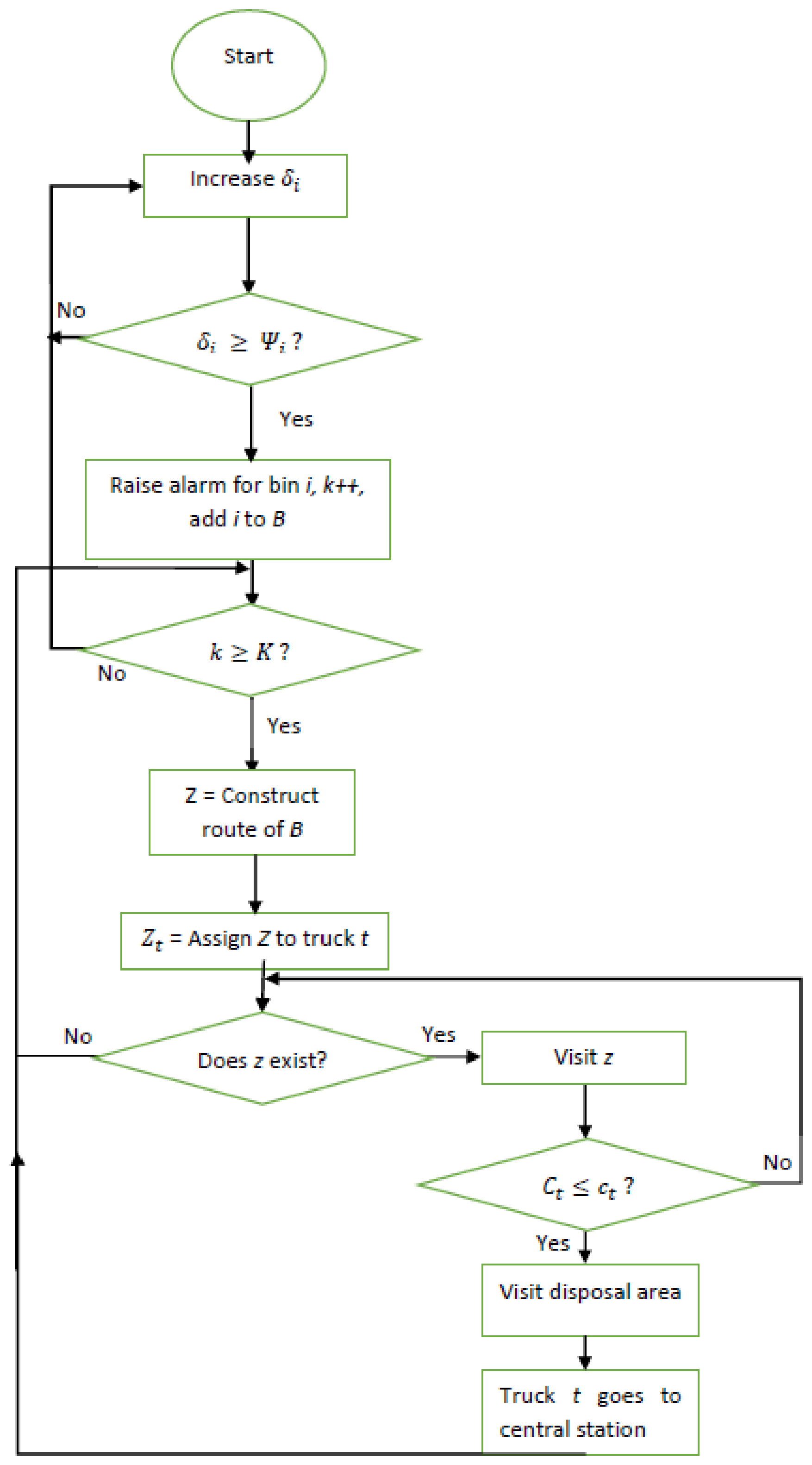
5.2.1. Collect based on Upper Threshold

The CUT model is constructed to address the problem of the waste management by providing an efficient route differently than CVF. This approach tries to reduce the cost by making the route more optimal. In this approach, visited bins are not only the ones that raised alarms, but also the ones that are on the assigned route and have not triggered the alarms. The reason behind this is to reduce the unnecessary trips of a truck to collect the waste from the bins.

The first part of CUT is constructed in the same way as CVF, which was presented earlier. Until the construction of the first route, the algorithm behaves in the same manner. While the CVF approach collects the closer bins that raised the alarms, the CUT method aims to collect the bins that are on the same assigned route even though they have not triggered the alarms. Trucks that visit the disposal area or that are assigned new routes operate in the same manner as in CVF. The flowchart of the CUT is presented in Figure 3.

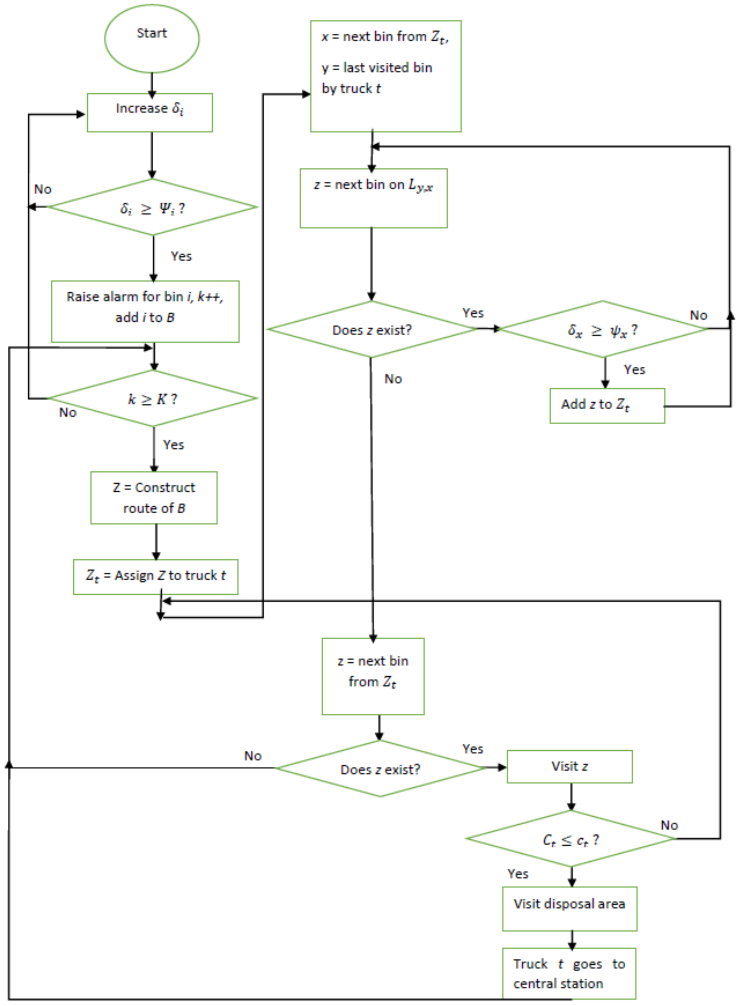
5.2.2. Collect based on Upper and Lower Threshold

The CULT model is developed to address the problem of the waste management by improving the efficiency of the route construction that was presented by the previous approaches. This approach tries to reduce the cost by making the route more optimal and removing unnecessary visits to the bins with an insignificant amount of waste. In this approach, visited bins are not only the ones that raised alarms, but also the ones that are on the way to the bins that generated alarms. However, different from the CUT approach, there is a decision point in order to visit a bin, which has not triggered an alarm. The reason behind this behaviour is to reduce the unnecessary service given to the passed-by bins that contain a negligible amount of waste. Hence, it aims at cost reduction. For the mentioned decision, a new parameter defining a lower threshold value for the waste amount (${\psi }_i$) is introduced.

CULT is constructed in the same manner as the CUT model presented previously. However, when truck i is assigned a route, it checks the bins that are accessible on the way from the current location to the next bin on the route. However, the decision about whether or not to add new bins on-the-fly depends on their current waste levels. Only the bins that are on the way and having a waste amount higher than ${\psi }_i$ are candidates for pick up by truck i. Trucks visiting the disposal area or those being assigned new routes follow the same steps as CVF and CUT. The flowchart of CUT is presented in Figure 4.

6. Performance Evaluation

The optimization toolbox in MATLAB has been used to solve both MILP models (cost and delay) [33]. The simulation environment for heuristic methods that are presented in this paper is a Java-based home-grown simulator. It is worth noting that the optimization models aim to provide a performance guideline for the heuristics and are not envisioned to be run in real-time scenarios. As a matter of fact, large map scenarios such as those with more than 15 bins would require fast heuristics as opposed to optimization models due to the high computational complexity of those formulations. In the next two subsections, detailed settings and results are presented along with a thorough discussion.

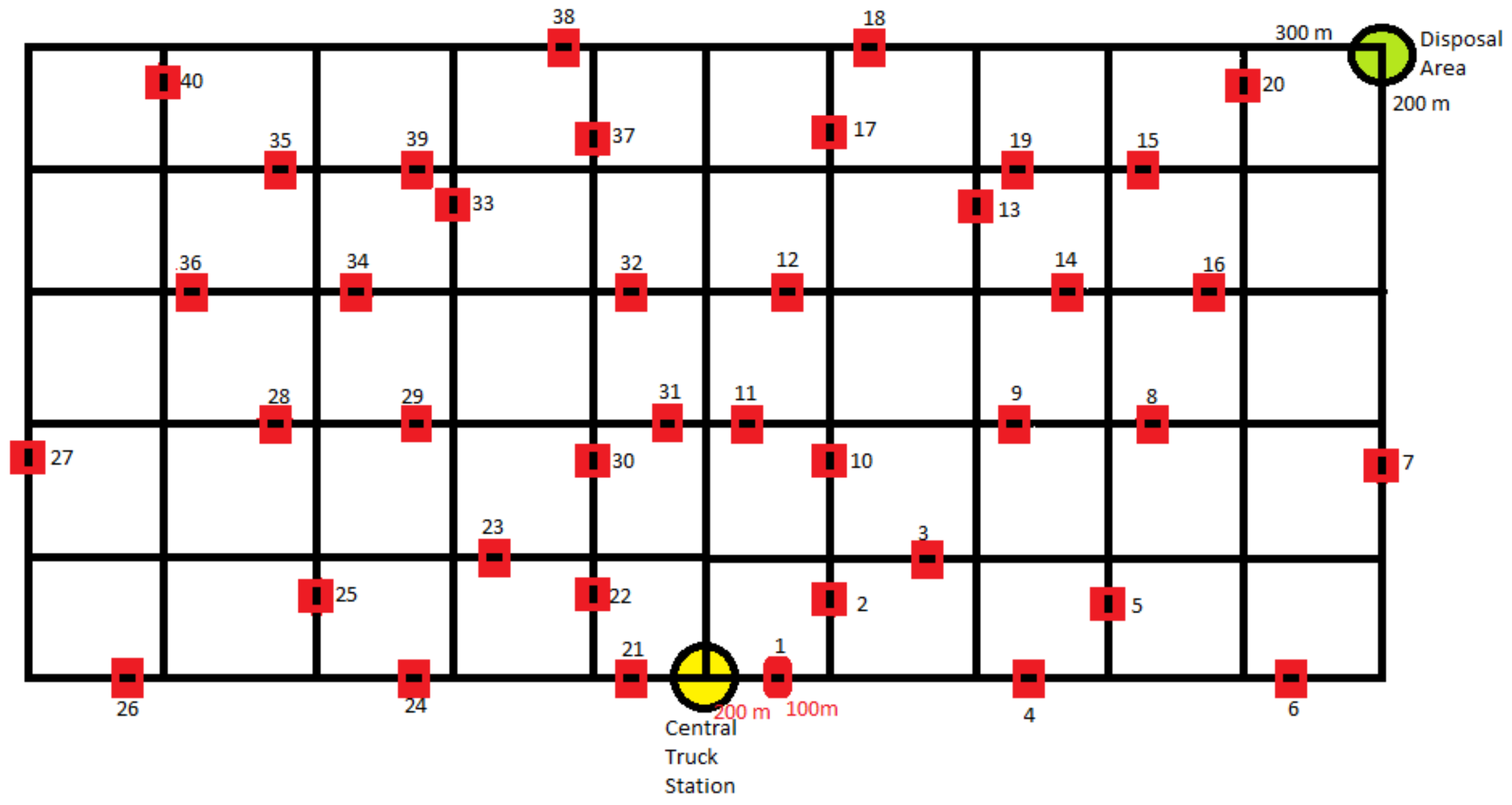
6.1. Simulation Settings

The simulation settings are given in

Table 2. Performance evaluation settings.

Notations	Value
Cost of emptying bin (D)	1.62 €/bin
Cost of human resource (H)	39 €/h
Cost of gas mileage (G)	20 €/km
Average speed in the town (S)	20 km/h
Time needed to collect waste from a bin (W)	2.5 min
Total number of trucks (N)	2
Total number of bins (M)	{5, 10, 15, 20, 40, 80, 160}
The upper bound of variable $P_i$ ($UB$)	10${}^{15}$
The upper threshold for the waste amount of bin i (${\mathsf{\Psi }}_i$)	[10–15] kg
The lower threshold for the waste amount of bin i (${\psi }_i$)	[5–8] kg
Penalty of the overflowed bin (${\rho }_i$)	5 €/kg
Time needed to empty truck t at the dumping area and prepare it for the next trip ($R_t$)	12 min
Distance from the dumping area to the central station (ℏ)	2500 m
Distance between bin i and bin j (${\Delta }_{ij}$)	[200–2300] m
Time needed to move from bin i to bin j ($t_{ij}$)	[0.6–6.9] min
Distance from bin i to the dumping area (${\Delta }_i$)	[400–2300] m
Distance from the central station to bin i ($r_i$)	[200–2300] m
Average waste arrival rate at a bin (${\lambda }_i$)	{1, 3, 5, 7} kg/5 min
Number of workers in a truck ($h_t$)	3
Maximum capacity of a bin (${\mathsf{\Lambda }}_i$)	{20, 30} kg
Initial load for bin i (${\delta }_i$)	[0–30] kg
Maximum capacity of a truck ($C_t$)	{400, 600} kg
Time from the central station to the first bin i ($T_i$)	[0.6–6.9] min
Initial load of a truck t ($c_t$)	[0–600] kg
Threshold for the count of bins that have alarmed (K)	{1,2,3}
Number of bins that have alarmed (k)	[0–160]
Alarm status of bin i ($A_i$)	{On, Off}

, and they describe the values used in the optimization models. The central station, which is the start and end point, hosts two trucks that participate in the waste collection process. Each truck has $h_t$ = 3 workers, who get paid H= 39 €/h, and moves with speed S = 20 km/h. In addition, the workers collect waste from a bin in W = 2.5 min with a cost D = 1.62 €/bin. Moreover, the truck gas mileage costs 20 €/km (i.e., G). Each truck goes to the landfill to empty the collected waste and prepare for the next bins’ alarm in 12 min (i.e., R${}_t$). The distance from the landfill area to the central station (ℏ) is set to 250 m. In the case of an overflowed bin, an additional cost of ${\rho }_i$ = 5 € is added as a penalty. However, a small map scenario with M = {5, 10, 15} bins and waste arrival rate ${\lambda }_i$ = {1, 3, 5, 7} kg/5 min was considered in order to compare the proposed approaches with both optimization models (cost and delay), as shown in Section 6.2.1. In the given scenario, the truck and the bin have a maximum capacity C${}_t$ = 400 kg and ${\mathsf{\Lambda }}_i$ = 20 kg, respectively. On the other hand, the larger map scenario considers $M\in$ {20, 40} bins, a waste arrival rate of ${\lambda }_i$ = {3 kg/5 min, 5 kg/5 min} and a bin capacity ${\mathsf{\Lambda }}_i\in$ {20 kg, 30 kg}, while the truck capacity (C${}_t$) takes its value from the set {400, 600} kg, as given in Section 6.2.2. Furthermore, in order to present our approaches’ suitability for the real case scenarios, the test scenarios are enhanced by getting results with larger maps considering M = {80, 160}, a waste arrival rate of ${\lambda }_i$= 3 kg/5min, ${\mathsf{\Lambda }}_i$= 30 kg, while a truck capacity (C${}_t$) = 600 kg, as given in Section 6.2.2.

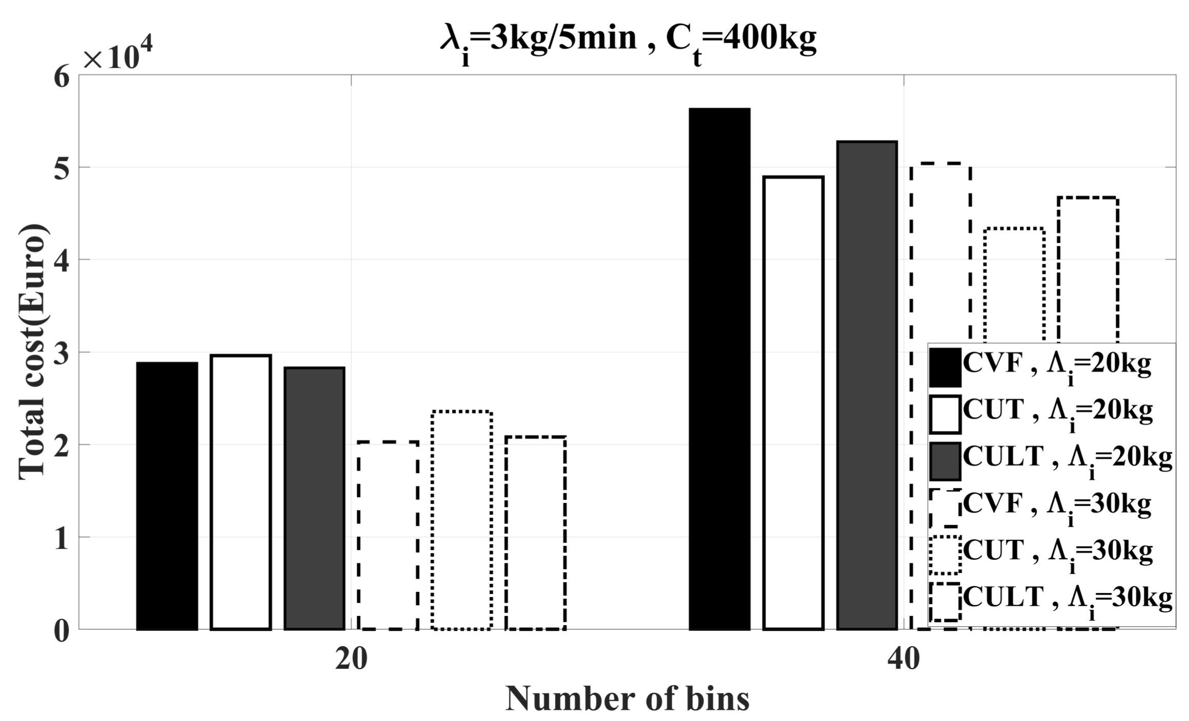
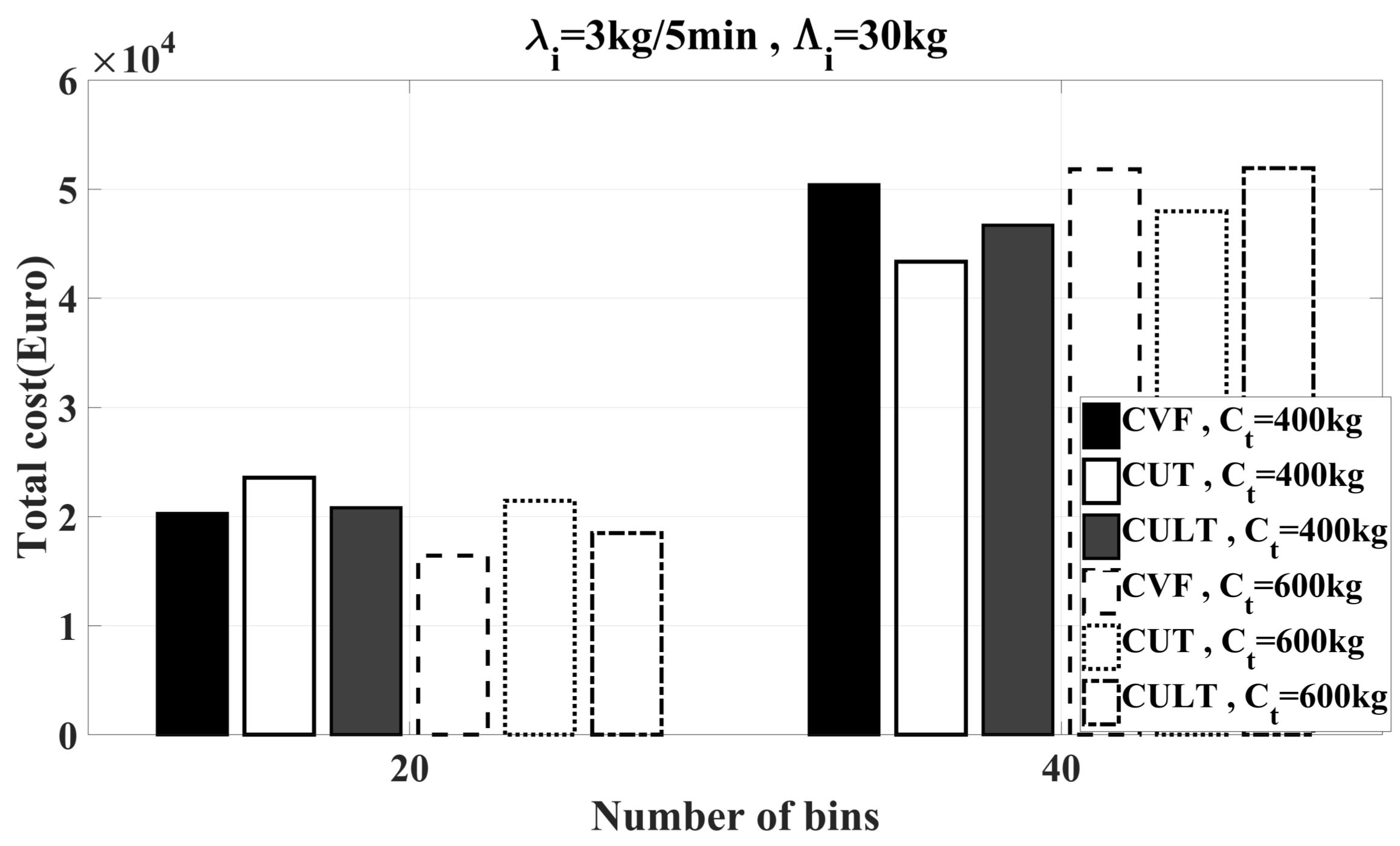
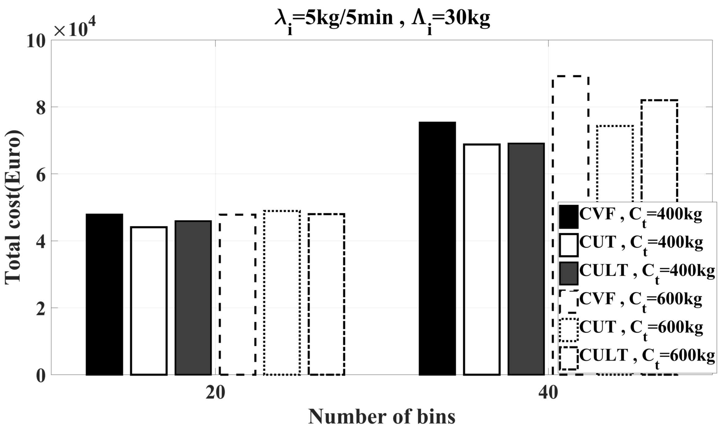
6.2. Simulation Results

In this section, the proposed waste collection approaches are evaluated to investigate how well the proposed solutions align with the optimization model results. The first subsection compares the two heuristics and the optimization model results for some small-scale scenarios. However, due to the inefficiency of the ILP solver under large maps, the second subsection shows more complex scenarios using larger maps and the comparison of the proposed heuristic approaches.

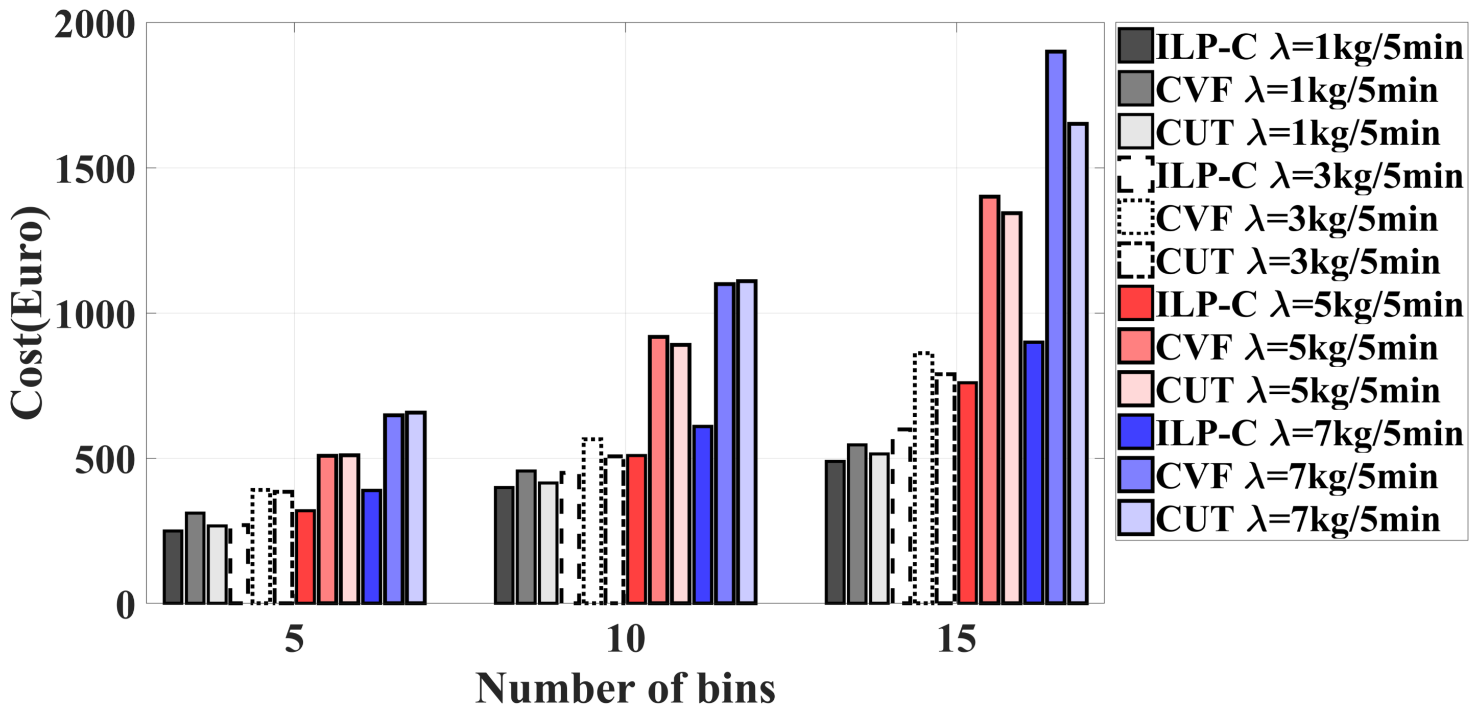
6.2.1. Optimality Assessment of the Heuristics

In order to evaluate the optimality of the proposed approaches, a comparison among the optimization model, CVF and CUT approaches is presented. Two criteria were considered in the comparison, namely the total cost and delay, as shown in Figure 5 and Figure 6, respectively. Moreover, the comparison shows the influence of changing the number of bins and the waste arrival rate on the cost value and delay time. Figure 5 presents the total cost for three different bin scenarios (i.e., the number of bins is either 5, 10 or 15) and four different waste arrival rates starting from lighter values to more aggressive values (1 kg/5 min, 3 kg/5 min, 5 kg/5 min and 7 kg/5 min). The results show that the cost increased either when the number of bins increased or the waste arrival rate became more aggressive. However, the CVF and CUT approaches became very close to the cost optimization result with an arrival rate of 1 kg/5 min for all bin scenarios. With higher waste arrival rates, the penalty value increased since the bins could end up overflowing rapidly. Hence, the gap between the optimal solution and the two heuristic approaches became larger particularly under the arrival rate of 5 kg/5 min and 7 kg/5 min. It is definitely not realistic to have such high arrival rates, so we would like to present how aggressive arrival rates significantly increased the cost due to the penalties.

A second criterion used to evaluate the proposed approaches was delay. To be coherent with the other performance comparisons, we considered the same bin scenarios (i.e., the number of bins is either 5, 10 or 15) and the same waste arrival rates (1, 3, 5 and 7) kg/5 min. Figure 6 shows the total delay of both trucks that participated in the waste collection process. In contrast to the cost model, the delay value was poorly affected by varying the waste arrival rate; however, varying the number of bins increased the total delay since the trucks needed more time to empty all the bins. The comparison shows that CUT had better results compared to CVF, particularly under the scenario with a higher number of bins. As a conclusion, both figures show that CUT is a better candidate in waste collection operation.

6.2.2. Feasibility Study of Heuristics

In order to compare the effectiveness and efficiency of the heuristic methods, several scenarios were applied to the simulation environment. In the simulation environment, the arrival process of the waste was formulated based on the Poisson distribution. Under multiple runs, distinct instances of the bins were obtained. For each scenario, the results were calculated as the average of five different runs.

For the comparisons, two maps, which included 20 and 40 bins, were used. The map containing 40 bins was two-times larger than the 20-bin map. The map with 40 bins is presented in Figure 7. On the map, the central truck station is where the trucks start their routes, and the disposal area is the point where trucks visit upon reaching their capacity upper limit. Each vertical segment of the grid is 200 m long, and each horizontal segment is 300 m long. Bins are marked with red rectangles on the map. In each scenario, two trucks were employed. Three different arrival rates, which were 1 kg per 5 min, 3 kg per 5 min and 5 kg per 5 min, were used. For these settings, increasing the bin capacity from 20 kg to 30 kg and increasing the truck capacity from 400 kg to 600 kg were observed separately. Each scenario was solved by the CVF, CUT and CULT methods. In order to compare these three methods, cost, delay per route and the number of trips values were used. Total cost was obtained for 12 h. Delay per route was obtained by dividing the total time that trucks needed to visit the bins by the route count for 12 h. Instead of total delay, the delay per route metric was employed.

In the first two figures, Figure 8 and Figure 9, cost values are observed under the arrival rate of 3 kg per 5 min. In the first figure, Figure 8, the change is observed for bin capacity being increased from 20 kg to 30 kg. In Figure 9, the impact of truck capacity being increased from 400 kg to 600 kg is depicted. The increase in the bin count improved CUT when compared to CULT and CVF. For the 20-bin case, both methods similarly increased their performance in comparison to CVF in terms of cost. Under the 40-bin case, CUT and CULT performed better than CVF and provided a more efficient solution in terms of cost. However, increasing bin capacity did not introduce further improvements to the performance CUT and CULT in comparison to CVF. CUT provided a 14% better solution than CVF, whereas CULT provided a 0.07% better solution than CVF. When the bin capacity increased, the difference between the threshold value that triggered the alarm and the bin capacity increased, as well. This resulted in trucks having a longer period of time to visit that bin before the waste started to spread and caused the penalty. Collecting the waste from the bins that have not yet triggered alarms caused longer delay values for the ones that had alarmed to be collected. This increased the penalty for CUT and CULT. When there was not enough time between the alarm threshold being reached and bin capacity being met, the decision mechanism can affect the solution by decreasing the total cost, and vice versa.

When increasing truck capacity under the 20-bin case in Figure 9, all three methods provided reasonable solutions. CVF performed the best, and for CUT and CULT, the difference from CVF increased in a negative way. Under the 40-bin case, CUT performed the best, and increasing truck capacity made CULT perform worse than CVF. Under the lower truck capacity, both CUT and CULT performed better than CVF. Moreover, the improvement of CVF by CUT decreased when the truck capacity was increased. Increasing truck capacity was expected to decrease the total cost in general depending on the trip count decrease and observed as expected for the map with 20 bins. However, when there were 40 bins on the map, increasing truck capacity caused higher cost values. This was due to the more non-optimal routes. The distance between bins could be higher in the wider area, and when the truck could not reach its capacity, it needed to wait for new triggers to be generated. This led to longer distances for the trucks to visit. Moreover, visiting further bins caused other bins on the route to spread waste around and cause penalties.

In the following two figures, Figure 10 and Figure 11, the change in bin capacity and truck capacity is studied under the arrival rate of 5 kg per 5 min. When the arrival rate increased, the results became closer to each other. The bins that did not trigger, but on the way of a truck that was assigned a route were highly probable to have generated a trigger at the next arrival of waste. Therefore, adding these kinds of bins independently of ${\psi }_i$ to the route increased the efficiency in terms of cost and delay. Moreover, selecting closer ${\mathsf{\Lambda }}_i$, $\lambda$, ${\mathsf{\Psi }}_i$ and ${\psi }_i$ resulted in similar cost and delay results. In the scenarios applied, ${\psi }_i$ was set to ${\mathsf{\Lambda }}_i$/4 and ${\mathsf{\Psi }}_i$ was set to ${\mathsf{\Lambda }}_i$/2. For ${\mathsf{\Lambda }}_i$ = 20, and $\lambda$ = 5 kg/5 min, ${\psi }_i$ = 5; when a bin received an amount of waste, it reached the ${\psi }_i$ directly. This removed the difference between CUT and CULT methods in this scenario. For the 5 kg/5 min arrival rate scenario, increasing bin capacity decreased the total cost for all methods, but did not have a significant impact on the comparison of the three algorithms.

However, increasing truck count caused a more significant impact on the cost values, which can be seen from Figure 11. Increasing truck capacity increased the total cost in general for both maps containing 20 and 40 bins. However, in the 40-bin case, the improvement of the CUT and CULT according to CVF increased. They both performed better in each situation, but they increased the efficiency percentages that they provided when compared to CVF.

The change in the settings provided less difference in delay when compared to cost values. Delay per route values was effected by how well the route was optimized and how close the visiting bins were. When the delay was decreased, it could be said that the route was more optimized in those simulations with the provided configuration settings. The following four figures are presented to show the comparison in terms of delay per route.

In Figure 12, the increasing bin capacity affect can be seen for the 20-bin and 40-bin maps with the arrival rate of 3 kg per 5 min. The impact was very small; however, in general, the CVF provided the shortest and CUT provided the longest delay per the route values. It is seen in Figure 8 that CUT was the most effective among the three algorithms on the 40-bin map. Therefore, CUT can be chosen as a solution when the time is not important, but the cost efficiency is more important. When time is the most important metric, CVF can be chosen. This was the result of CUT providing more optimal routes for each truck. Since trucks visited any other bin on the way to the alarmed bins, trucks did not have to go further first and come back again for the bins that they passed by before. Furthermore, when the bin count was increased, the delay per route values decreased, and this meant that the algorithms could work better and manage more optimal routes when the area was wider and there were more triggers coming from the bins in a time window. When there were less bins on the map, the possibility of getting many triggers at the same time decreased, and getting less triggers would cause the bins to be added on the route in an unoptimized manner.

In Figure 13, the increase in truck capacity can be seen at the arrival rate of 3 kg per 5 min. It is observed that when the truck capacity was increased, the delay per route increased. This is precisely the expected result to be observed, since there was more capacity that one truck could collect, and it visited more bins in a route. Moreover, increasing truck capacity resulted in more effective performance of CVF and less effective performance of CULT, which was the opposite condition of the lower truck capacity scenario.

In the following figures, Figure 14 and Figure 15, the scenarios where the arrival rate was 5 kg/5min are presented. The delay per route values was smaller in general when compared to Figure 12 and Figure 13. Since the arrival rate was increased, the collected bins had higher amount of wastes stored in them. This resulted in a shorter time for the trucks reaching their capacity. In Figure 14, the affect of bin capacity increase is shown. Increasing the truck capacity effected smaller map scenarios more than the wider area map. In the first section on the left, the biggest impact can be observed by the CULT, and while CULT and CVF were performing better, CUT increased the delay per route value for the smaller area case. For the wider area, all the methods performed better and provided smaller delay values when the bin capacity was increased.

In Figure 15, the effect of truck capacity increase is shown. The increase in delay per route values in all cases where the truck capacity was increased independently of other configuration settings was the natural result. For this figure, where the arrival rate was 5 kg/5min and the bin capacity was 30 kg, increasing the truck capacity from 200 kg to 400 kg did not change the order of the effectiveness of the three algorithms. CVF provided the smallest delay per route values, and CUT provided the longest ones.

As the last comparison metric, the number of routes in each scenario are shown in the following four figures.

In Figure 16 and Figure 17, the arrival rate is 3 kg/5 min, and the simulation is observed for 20 bins and 40 bins maps. First, in Figure 16, the increase in bin capacity is presented. The highest route number was always in CVF, and the lowest was in CUT. However, the difference between the methods is more visible and observable when the wider map was used. Route count being small meant that each trip took a longer time for that method, and a trip took longer when the bins either had a small amount of waste inside in each collection or the routes that the trucks were assigned to were not that optimal. The increase in the bin capacity increased the number of routes in both cases when there were 20 or 40 bins. The reason behind this behaviour was that the thresholds were set according to the bin capacities (${\mathsf{\Lambda }}_i$’s), which is $\mathsf{\Lambda }$/2. Once an alarm has been triggered, the bin had a greater amount of waste to be collected. This consumed the truck capacity more quickly and resulted in higher values of route counts.

In Figure 17, the increase in the truck capacity is presented. In this figure, like the previous one, CUT had the smallest number of routes, and CVF had the most number of routes. Again, the difference among them is more visible when the map has 40 bins. For both maps, when the truck capacity increased, the route number decreased. With the increased truck capacity, one truck could hold more waste in a single trip, which precisely resulted in the decrease in the number of routes.

For the following two figures, Figure 18 and Figure 19, the arrival rate is set to 5 kg/5 min, and the maps with 20 and 40 bins are observed under increasing bin capacity or truck capacity. First, in Figure 18, the increase in the bin capacity is observed.

In Figure 19, the increase in the truck capacity is tested under the 5 kg/5 min arrival rate setting. The increase in the truck capacity decreased the count of routes as explained before. For these scenarios, again, the highest number of routes was observed by applying CVF, whereas the lowest number of routes were observed under CUT and CULT.

In the following

Table 3. Cost when $\lambda$ = 1 kg/5 min.

Method	Bin Count	Bin Capacity (kg)	Truck Capacity (kg)	Cost (€)	Delay per Route	No. of Routes
$CVF$	20	20	400	5354.16	193.78	5.8
$CUT$	20	20	400	6246.67	205.16	6
$CULT$	20	20	400	5542.85	199.41	5.8
$CVF$	20	30	400	4343.99	155.17	5.8
$CUT$	20	30	400	4953.32	187.85	5.6
$CULT$	20	30	400	4229.57	143.68	6.2
$CVF$	20	30	600	4189.10	305.8	2.8
$CUT$	20	30	600	4936.05	345.12	3
$CULT$	20	30	600	4134.74	330.23	2.6
$CVF$	40	20	400	11,188.28	109.36	12
$CUT$	40	20	400	14,950.88	126.79	10
$CULT$	40	20	400	11,801.55	112.27	11.6
$CVF$	40	30	400	5926.93	104.85	12
$CUT$	40	30	400	11,722.18	116.95	10.4
$CULT$	40	30	400	6634.55	104.22	12
$CVF$	40	30	600	5665.45	158.35	8
$CUT$	40	30	600	11,579.94	17,726	7
$CULT$	40	30	600	6066.07	157.86	8

, total cost, delay per route and number of route counts are presented when $\lambda$ = 1 kg/5 min. The applied scenarios are the same as the previous cases. The increase in ${\mathsf{\Lambda }}_i$ and $C_i$ were tested on two maps containing 20 and 40 bins.

In Table 3, the first part presents the results on the map with 20 bins. When ${\mathsf{\Lambda }}_i$ and $C_i$ were lower, the CVF results were more efficient in terms of cost. However, increasing these parameters separately resulted in more efficient solutions when compared to CULT. Since $\lambda$ was small, there was enough time for the trucks to visit bins that had alarmed and collect the ones on their way according to the decision mechanism in CULT. Delay per route values were similar for CVF and CULT in most cases. As the truck capacity increased, the difference between them started to become wider. In addition, CUT yielded longer durations for a single trip in each scenario on the smaller map. The number of routes was quite similar on the smaller map. Comparing the methods for this particular performance metric on the wider map was more worthwhile.

When the simulation scenarios were tested on the map with 40 bins, CVF demonstrated the most competent performance, whereas CUT resulted in the worst solutions in terms of cost. Increasing ${\mathsf{\Lambda }}_i$ and $C_i$ also increased the gap between CVF and its counterparts. Delay per route under CVF and that under CULT on the wider map were quite similar. CUT exhibited a longer delay time per route, which meant adding new bins on-the-fly ended up increasing the delay by collecting waste from bins that did not have a significant amount of waste accumulated. Delay per route may not significantly change when the bin capacity was increased. Thus, trip durations mostly depended on the truck capacity. Similar to the delay performance, the number of routes that trucks had in a single simulation run was smaller under CUT. Since trucks travelled longer in a single trip and the total delay did not change significantly, the number of routes was smaller under CUT. Moreover, the route numbers almost never changed under CVF and CULT. Besides, increasing the truck capacity had a direct impact on the route count, but not the bin capacity.

In order to present our approaches’ suitability to real-life scenarios, the test scenarios were modified to show results with larger maps that contained more bins. Three additional larger maps were used: (1) the map given in Figure 7 for the 40-bin scenario was modified, and 40 more bins (total of 80 bins) were deployed to the region; (2) the map given in Figure 7 was duplicated in terms of the area and the number of bins; moreover, a third map of 160 bins was constructed. All three approaches (i.e., CVF, CUT and CULT) were tested using these three maps with the following parameter settings: bin capacity (${\mathsf{\Lambda }}_i$ = 30 kg), truck capacity (C${}_t$ = 600 kg), waste arrival rate (${\lambda }_i$ = 3 kg/5min) and the number of trucks (N= 2). These scenarios were compared based on their total cost, delay per route and the number of routes. The results are presented in Figure 20, Figure 21 and Figure 22.

Figure 20 shows the total cost obtained under these three scenarios. CUT outperformed its counterparts, CULT and CVF. As mentioned earlier in this section, under the moderate arrival rate, as the map became larger, CUT tended to provide more cost-efficient solutions. As expected, increasing map size and the number of bins increased the total cost for all methods. Definitely, the higher the number of bins, the higher the number of triggers during a certain period of time. On the other hand, by considering more triggers when making decisions, the routes could be constructed more efficiently (leading to consecutively visited bins becoming closer). Hence, better cost values were achieved, and as we increased the area, we did not observe a remarkable increase in the total cost values obtained.

Figure 21 and Figure 22 present the delay per route and the number of routes, respectively, calculated for the same three scenarios. In terms of total delay, CUT provided the most efficient results for all three scenarios with two trucks. However, the number of routes was the lowest for CUT and highest for CVF. Moreover, total delay did not change significantly as observed for the previous cases. Hence, CVF resulted in the smallest delay per route. Previously, it was observed that the delay per route decreased as the area became larger due to the increase in the route counts. The results of 80-bin and 160-bin scenarios also supported this. As the number of routes increased, shorter routes were established since collected bins became closer to each other and the trucks reached their capacity limits quickly.

As for the complexities of these three methods, the Big O notation is applied. All three methods use Dijkstra’s algorithm to generate the shortest path from the given weighted adjacency matrix. The weights are the distances between the nodes, which represent the bins. Dijkstra’s algorithm calculates the shortest distance, but does not calculate the path information. It is modified for the simulation environment to show the shortest path between any given two nodes for the methods CUT and CULT. At the beginning of the simulation, Dijkstra’s algorithm runs and constructs a matrix representing the distances between any two points. For CUT and CULT, an additional matrix representing the path information between any two nodes is constructed. Dijkstra’s algorithm is not covering to negative weighted edges, and Bellman–Ford algorithm can be used in that case and improve the constructed route for a truck in the simulation environment. The time complexity of Dijkstra’s algorithm is $O\left(V^2\right)$, where V denotes the number of vertices in a connected graph.

If binary heap representation were used, it might have improved the complexity and have reduced it to $O\left(ElogV\right)$, E being the edge count and V being the number of vertices. This complexity is for constructing the matrices at the beginning. Time complexity for adding a bin to the route is $O\left(M\right)$, M representing the bin count. Time complexity for checking the bins on the shortest path in CUT and CULT is $O\left(M\right)$. In summary, all three methods have the time complexity of $O\left(V^2\right)$, where V denotes the number of vertices in a connected graph.

According to the results, when the bin capacity and bin threshold’s (${\mathsf{\Psi }}_i$, ${\delta }_i$) had a high difference compared to each other, in the small sized area with smaller arrival rates ($\lambda$), CVF gave a more efficient solution compared to CUT and CULT. This means there was enough time for the trucks to reach the bins that raised alarms before waste was spread on the ground. The penalty values for spread waste affected the total cost in terms of the spread waste amount. In this situation, collecting the waste from the bins that did not raise an alarm, even if they were on the way of the truck, increased the total cost and delay values since dumping a single bin had its own cost and time consumption. CUT gave the least efficient solution among them. CULT provided a better solution and became closer to the the solution of CVF if the truck capacity also increased. This was the result of a decrease in the number of trips to the disposal area. When truck capacity was higher, the trucks could pick up more bins in one trip. The additional bins that did not raise an alarm, but were picked up on the way did not occupy a significant amount of space in the truck when $C_i$ was higher. It is worth noting that the longest path was the ones between the disposal area and the central station (h), and also, the most time-consuming activity was emptying the waste at the disposal area and making the truck ready for the next trip ($R_t$), so increasing the trip count increased the cost and delay significantly.

In larger maps, with higher ${\mathsf{\Lambda }}_i$ and proportional $\lambda$, the proposed heuristic CULT provided more efficient solutions regarding cost and delay. However, when the constants became closer and the map became smaller, CVF and CUT tended to ensure better solutions. The increase in the $C_i$ had more impact on the results when the map and the $\lambda$ were larger.

7. Conclusions

Wireless sensor and actuator networks in smart cities are essential for acquiring unique data that should be processed, analysed and used for decision-making/support systems that can improve the quality of life for the citizens. Among smart city services and applications, waste management has been challenging, and emergent, since its impacts are two-fold: quality of living and municipal costs.

In this paper, we have proposed a framework that aims at providing a sensor-driven waste management system by mainly providing trajectory assistance for the municipal agents (i.e., vehicles such as trucks) that are deployed for waste collection. In the proposed waste management system, a passive sensor is deployed in a particular bin to monitor the waste level. Besides the dedicated sensors, a cloud platform is responsible for the collection of the acquired sensor data, pre-processing, analysing and possibly presenting them to the end user. In the case of an exceeded threshold of the waste level, an actuator raises an alarm indicating the need to schedule a pickup. The pickup process is not as straightforward due to the following reasons: (1) Alarms may be triggered by multiple actuators; thus, the cloud platform, where sensory reports, as well as alarms are received and processed, is expected to run a schedule. (2) As the deployment of municipal agents is a costly process, the platform has to decide on whether or not to collect the waste in the bins that have not reached the pickup threshold yet. To address these problems, we have formulated two ILP models to form lower bounds in terms of the delay and cost performance. Furthermore, in order to emulate the behaviour of the ILP formulations, a greedy algorithm, Closest Vehicle First (CVF), and two heuristic solutions have been proposed, namely Collect based on Upper Threshold (CUT) and Collect based on Upper and Lower Threshold (CULT). The former defines an empirical upper threshold for collections, whereas the latter further checks whether the load level of a bin is below a lower threshold so as to postpone the collection process to an upcoming alarm. Through simulations, we have shown that the ILP formulations can provide cost and delay lower bounds for all three algorithms. Furthermore, the proposed heuristics CUT and CULT can reduce the cost under the greedy pickup schedule by (up to) 16.7% and 8.3% in the presence of a small number of bins. Moreover, under the same settings, we have also shown that CUT and CULT can reduce the delay of the greedy pickup by 4.6% and 3% in terms of delay, respectively. Last but not least, the greedy heuristic CVF is more favourable in large-scale scenarios when the covered region has 20 of more bins regardless of the waste arrival rate. As mentioned earlier, the optimization models are employed in urban areas, relying on reasonable waste arrival rates for the cities. Therefore, it is rare to have accumulative wastes in the bins for multiple consecutive days. Furthermore, Equations (13) and (36) ensure that all bins must be collected. Moreover, CUT ensures that all the bins, regardless of having raised alarms, on the same assigned route to the truck will be collected along with those residing on the same route. However, the model can be extended to include rural areas with very low arrival rates by adding a time counter for those bins that have not been collected for more than T days, where T can be set by the operator.

Our ongoing and future agenda includes multiple directions. Currently, we are working on building a multi-objective optimization and heuristics to meet various targets with the same decision support system. In the medium run, we will also integrate the latency and reliability of communication between the dedicated sensors and the cloud platform. In a longer time frame, we will develop an all-in-one integrated system that takes communication constraints, as well as financial- and user experience-related parameters into account. Moreover, the model can be extended to include rural areas with very low arrival rates by adding a time counter for those bins that have not been collected for more than T days, where T can be set by the operator.

References

1. Habibzadeh, H.; Qin, Z.; Soyata, T.; Kantarci, B. Large Scale Distributed Dedicated- and Non-Dedicated Smart City Sensing Systems. IEEE Sens. J. 2017, 17, 7649–7658. [Google Scholar] [CrossRef]
2. Shyam, G.K.; Manvi, S.S.; Bharti, P. Smart waste management using Internet-of-Things (IoT). In Proceedings of the 2nd International Conference on Computing and Communications Technologies (ICCCT), Chennai, India, 23–24 February 2017; pp. 199–203. [Google Scholar]
3. Habibzadeh, H.; Boggio-Dandry, A.; Qin, Z.; Soyata, T.; Kantarci, B.; Mouftah, H.T. Soft Sensing in Smart Cities: Handling 3Vs Using Recommender Systems, Machine Intelligence, and Data Analytics. IEEE Commun. Mag. 2018, 56, 78–86. [Google Scholar] [CrossRef]
4. Page, A.; Hijazi, S.; Askan, D.; Kantarci, B.; Soyata, T. Research Directions in Cloud-Based Decision Support Systems for Health Monitoring Using Internet-of-Things Driven Data Acquisition. Int. J. Serv. Comput. 2016, 4, 18–34. [Google Scholar]
5. Pouryazdan, M.; Kantarci, B.; Soyata, T.; Song, H. Anchor-Assisted and Vote-Based Trustworthiness Assurance in Smart City Crowdsensing. IEEE Access 2016, 4, 529–541. [Google Scholar] [CrossRef]
6. Pouryazdan, M.; Kantarci, B. The Smart Citizen Factor in Trustworthy Smart City Crowdsensing. IT Prof. 2016, 18, 26–33. [Google Scholar] [CrossRef]
7. Hijazi, S.; Page, A.; Kantarci, B.; Soyata, T. Machine Learning in Cardiac Health Monitoring and Decision Support. IEEE Comput. 2016, 49, 38–48. [Google Scholar] [CrossRef]
8. Silva, B.N.; Khan, M.; Han, K. Towards sustainable smart cities: A review of trends, architectures, components, and open challenges in smart cities. Sustain. Cities Soc. 2018, 38, 697–713. [Google Scholar] [CrossRef]
9. Atzori, L.; Iera, A.; Morabito, G. Understanding the Internet of Things: Definition, potentials, and societal role of a fast evolving paradigm. Ad Hoc Netw. 2017, 56, 122–140. [Google Scholar] [CrossRef]
10. Strzelecka, A.; Ulanicki, B.; Koop, S.; Koetsier, L.; van Leeuwen, K.; Elelman, R. Integrating Water, Waste, Energy, Transport and ICT Aspects into the Smart City Concept. Procedia Eng. 2017, 186, 609–616. [Google Scholar] [CrossRef]
11. Gruler, A.; Quintero-Araújo, C.L.; Calvet, L.; Juan, A.A. Waste collection under uncertainty: A simheuristic based on variable neighbourhood search. Eur. J. Ind. Eng. 2017, 11, 228–255. [Google Scholar] [CrossRef]
12. Aazam, M.; St-Hilaire, M.; Lung, C.H.; Lambadaris, I. Cloud-based smart waste management for smart cities. In Proceedings of the IEEE 21st International Workshop on Computer Aided Modelling and Design of Communication Links and Networks (CAMAD), Toronto, ON, Canada, 23–25 October 2016; pp. 188–193. [Google Scholar]
13. Coban, A.; Ertis, I.F.; Cavdaroglu, N.A. Municipal solid waste management via multi-criteria decision making methods: A case study in Istanbul, Turkey. J. Clean. Prod. 2018, 180, 159–167. [Google Scholar] [CrossRef]
14. Minghua, Z.; Xiumin, F.; Rovetta, A.; Qichang, H.; Vicentini, F.; Bingkai, L.; Giusti, A.; Yi, L. Municipal solid waste management in Pudong New Area, China. Waste Manag. 2009, 29, 1227–1233. [Google Scholar] [CrossRef] [PubMed]
15. Fussa, M.; Barros, R.T.V.; Poganietz, W.R. Designing a framework for municipal solid waste managementtowards sustainability in emerging economy countries—An application to a case study in Belo Horizonte (Brazil). J. Clean. Prod. 2018, 178, 655–664. [Google Scholar] [CrossRef]
16. Ikhlayel, M. Development of management systems for sustainable municipal solid waste in developing countries: A systematic life cycle thinking approach. J. Clean. Prod. 2018, 180, 571–586. [Google Scholar] [CrossRef]
17. Guerrero, L.A.; Maas, G.; Hogland, W. Solid waste management challenges for cities in developing countries. Waste Manag. 2013, 33, 220–232. [Google Scholar] [CrossRef] [PubMed]
18. Marshall, R.E.; Farahbakhsh, K. Systems approaches to integrated solid waste management in developing countries. Waste Manag. 2013, 33, 988–1003. [Google Scholar] [CrossRef] [PubMed]
19. Henry, R.K.; Yongsheng, Z.; Jun, D. Municipal solid waste management challenges in developing countries—Kenyan case study. Waste Manag. 2006, 26, 92–100. [Google Scholar] [CrossRef] [PubMed]
20. Anagnostopoulos, T.; Kolomvatsos, K.; Anagnostopoulos, C.; Zaslavsky, A.; Hadjiefthymiades, S. Assessing dynamic models for high priority waste collection in smart cities. J. Syst. Softw. 2015, 110, 178–192. [Google Scholar] [CrossRef] [Green Version]
21. Manqele, L.; Adeogun, R.; Dlodlo, M.; Coetzee, L. Multi-objective decision-making framework for effective waste collection in smart cities. In Proceedings of the Global Wireless Summit (GWS), Cape Town, South Africa, 15–18 October 2017; pp. 155–159. [Google Scholar]
22. UNEP—United Nations Environment Programme. Municipal Solid Waste: Is it Garbage or Gold? 2013. Available online: https://na.unep.net/geas/getUNEPPageWithArticleIDScript.php?article_id=105 (accessed on 10 March 2018).
23. Johansson, O.M. The effect of dynamic scheduling and routing in a solid waste management system. Waste Manag. 2006, 26, 875–885. [Google Scholar] [CrossRef] [PubMed]
24. Jouhara, H.; Czajczyńska, D.; Ghazal, H.; Krzyzynska, R.; Anguilano, L.; Reynolds, A.; Spencer, N. Municipal waste management systems for domestic use. Energy 2017, 139, 485–506. [Google Scholar] [CrossRef]
25. Nuortioa, T.; Kytöjoki, J.; Niskaa, H.; Braysy, O. Improved route planning and scheduling of waste collection and transport. Expert Syst. Appl. 2006, 30, 223–232. [Google Scholar] [CrossRef]
26. Arebey, M.; Hannan, M.; Begum, R.; Basri, H. Solid waste bin level detection using gray level co-occurrence matrix feature extraction approach. J. Environ. Manag. 2012, 104, 9–18. [Google Scholar] [CrossRef] [PubMed]
27. Chenga, S.; Chanb, C.; Huang, G. An integrated multi-criteria decision analysis and inexact mixed integer linear programming approach for solid waste management. Eng. Appl. Artif. Intell. 2006, 16, 543–554. [Google Scholar] [CrossRef]
28. Mamun, M.A.A.; Hannan, M.A.; Hussain, A.; Basri, H. Theoretical model and implementation of a real time intelligent bin status monitoring system using rule based decision algorithms. Expert Syst. Appl. 2016, 48, 76–88. [Google Scholar] [CrossRef]
29. Apaydin, O. Route optimization for solid waste collection: Trabzon (Turkey) case study. Glob. NEST J. 2007, 9, 6–11. [Google Scholar]
30. Ramos, T.R.P.; de Morais, C.S.; Barbosa-Póvoa, A.P. The smart waste collection routing problem: Alternative operational management approaches. Expert Syst. Appl. 2018, 103, 146–158. [Google Scholar] [CrossRef]
31. Ramson, S.J.; Moni, D.J. Wireless sensor networks based smart bin. Comput. Electr. Eng. 2017, 64, 337–353. [Google Scholar] [CrossRef]
32. Data analytics approach to create waste generation profiles for waste management and collection. Waste Manag. 2018, 77, 477–485.
33. MATLAB Optimization Toolbox, version 8.0 (MATLAB R2017b). Available online: https://www.mathworks.com/products/optimization.html (accessed on 10 March 2018).
Figure 1. An overview of the system model.
Jsan 07 00029 g001
Figure 2. Closest Vehicle First (CVF) flowchart.
Jsan 07 00029 g002
Figure 3. Collect based on Upper Threshold (CUT) flowchart.
Jsan 07 00029 g003
Figure 4. Collect based on Upper and Lower Threshold (CULT) flowchart.
Jsan 07 00029 g004
Figure 5. An overview of the system model.
Jsan 07 00029 g005
Figure 6. An overview of the system model.
Jsan 07 00029 g006
Figure 7. Bin deployment map.
Jsan 07 00029 g007
Figure 8. Cost: bin count when the bin capacity was increased.
Jsan 07 00029 g008
Figure 9. Cost: bin count when the truck capacity was increased.
Jsan 07 00029 g009
Figure 10. Cost: bin count when the bin capacity was increased.
Jsan 07 00029 g010
Figure 11. Cost: bin count when the truck capacity was increased.
Jsan 07 00029 g011
Figure 12. Delay per route: bin count when the bin capacity was increased.
Jsan 07 00029 g012
Figure 13. Delay per route: Bin count when the truck capacity was increased.
Jsan 07 00029 g013
Figure 14. Delay per route: bin count when the bin capacity was increased.
Jsan 07 00029 g014
Figure 15. Delay per route: bin count when the truck capacity was increased.
Jsan 07 00029 g015
Figure 16. Number of routes: bin count when the bin capacity was increased.
Jsan 07 00029 g016
Figure 17. Number of routes: bin count when the truck capacity was increased.
Jsan 07 00029 g017
Figure 18. Number of routes: bin count when the bin capacity was increased.
Jsan 07 00029 g018
Figure 19. Number of routes: bin count when the truck capacity was increased.
Jsan 07 00029 g019
Figure 20. Cost: bin count as the number of bins increased.
Jsan 07 00029 g020
Figure 21. Delay per route: bin count as the number of bins increased.
Jsan 07 00029 g021
Figure 22. Number of routes: bin count as the number of bins increased.
Jsan 07 00029 g022