Design and Analysis of Adaptive Hierarchical Low-Power Long-Range Networks


1
Department of Computer Engineering and Informatics, University of Patras, 26504 Patras, Greece
2
Department of Computer, Control and Management Engineering “Antonio Ruberti”, Sapienza University of Rome, 00185 Rome, Italy
*
Author to whom correspondence should be addressed.
J. Sens. Actuator Netw. 2018, 7(4), 51; https://doi.org/10.3390/jsan7040051
Submission received: 15 October 2018
/
Revised: 16 November 2018
/
Accepted: 21 November 2018
/
Published: 27 November 2018
(This article belongs to the Special Issue Sensor and Actuator Networks: Feature Papers)
Abstract
:A new phase of evolution of Machine-to-Machine (M2M) communication has started where vertical Internet of Things (IoT) deployments dedicated to a single application domain gradually change to multi-purpose IoT infrastructures that service different applications across multiple industries. New networking technologies are being deployed operating over sub-GHz frequency bands that enable multi-tenant connectivity over long distances and increase network capacity by enforcing low transmission rates to increase network capacity. Such networking technologies allow cloud-based platforms to be connected with large numbers of IoT devices deployed several kilometres from the edges of the network. Despite the rapid uptake of Long-power Wide-area Networks (LPWANs), it remains unclear how to organize the wireless sensor network in a scaleable and adaptive way. This paper introduces a hierarchical communication scheme that utilizes the new capabilities of Long-Range Wireless Sensor Networking technologies by combining them with broadly used 802.11.4-based low-range low-power technologies. The design of the hierarchical scheme is presented in detail along with the technical details on the implementation in real-world hardware platforms. A platform-agnostic software firmware is produced that is evaluated in real-world large-scale testbeds. The performance of the networking scheme is evaluated through a series of experimental scenarios that generate environments with varying channel quality, failing nodes, and mobile nodes. The performance is evaluated in terms of the overall time required to organize the network and setup a hierarchy, the energy consumption and the overall lifetime of the network, as well as the ability to adapt to channel failures. The experimental analysis indicate that the combination of long-range and short-range networking technologies can lead to scalable solutions that can service concurrently multiple applications.
1. Introduction, Related Work and Our Approach
A plethora of small-factor devices with networking, computation and sensing capabilities are embedded in the physical world and interconnect it with the digital world of the Internet, creating the “Internet of Things” (IoT). Such networked devices are continuously deployed to accomodate the needs of different application domains, and, as a result, they have already surpassed the number of computers and mobile phones operated by humans. All these devices connected to the Internet enable an entirely new type of application and services that clearly affect all aspects of business and living.
One fundamental aspect of IoT is the networking technologies that allow the communication between the embedded devices and the Internet cloud services. For this reason, all the efforts up until now focused predominantly on wireless low-power transmission technologies such as IEEE 802.15.4 (ZigBee, Z-Wave) and IEEE 802.15.11 (Bluetooth, BLE) [1]. These technologies provide reasonably high bit rate exchanges over a short range. Due to this low-power and short-range mode of operation, deploying a large-sized network requires the use of communication protocols that deliver messages based on a multi-path approach [2]. Such a multi-path approach provides certain benefits, such as the capability to overcome communication obstacles [3,4], and the overall improvement of security of the network [5]. Experimentation over real-world wireless sensor networks has highlighted the difficulties and limitations of the multi-hop short-range paradigm [6]. In order to overcome these technical difficulties, several alternative solutions have been proposed, for example, by varying the transmission range of the nodes [4], providing hierarchical network structures [7] or even employing mobile nodes to facilitate network management [8]. Despite all these efforts, the reduced transmission range creates several difficulties that are difficult to overcome. As a result, real-world deployments need to use a combination of networking technologies in order to deliver urban-scale coverage in the context of smart city services [9,10].
Recently, a new approach has been proposed that exploits sub-GHz communication, which allows for transmitting over longer distances, and very low data transmission rates, which allow for reducing significantly power consumption [11]. This approach of network has been titled Low-Power Wide Area Networks (LPWANs) as apposed to short-range high-frequency communication. Low-frequency signals are not as attenuated by thick walls or multi-path propagation as high-frequency signals contributing in this way to robustness and reliability of the signal [12]. In LPWAN, the embedded devices are connected to Concentrators (also called a collector or concentrator) that are located several kilometres away. Evidently, LPWANs provide multiple benefits for IoT deployments, providing higher autonomy due to the reduced energy consumption, and decrease deployment costs as a small number of concentrators is required [12].
LPWAN uses proprietary modulation techniques that are derivatives of the Chirp Spread Spectrum (CSS) and operate in the sub-GHz bands. It allows end-nodes to communicate independently and asynchronously, similarly to an ALOHA-protocol. As a result, an LPWAN concentrator can receive data on the same channel from multiple IoT devices at the same time if the bit rates are different. This increases the capacity of nodes in a LPWAN. However, due to restrictions of the low duty cycle regulations in the unlicensed sub-GHz bands, LPWAN creates asymmetric situations where concentrators that are connected to a large number of IoT devices will be able to send downstream messages (i.e., messages arriving from the network servers to the IoT devices) less frequently to each node than a concentrator handling fewer IoT devices. Existing designs foresee both IoT devices and concentrators to transmit only 1% of the time to achieve low power consumption and high deployment numbers. On top of that, since IoT devices are operating in a low-power mode, listening to the communication channel for down-link messages is done occasionally, also severely limiting downstream message exchanges. Keeping in mind that many of the proposed applications require the deployment of very large number of devices, it is critical to propose certain extensions to existing LPWAN structures so that they can eventually accommodate very dense deployments of IoT devices without exceeding the capacity of the LPWAN [13,14].
Typical examples of dense IoT deployments can be easily identified in the remote metering and monitoring domain like [9,15,16,17]. Installation scenarios like this could include hundreds of connected meters installed deep inside buildings close to each other including both up-link and down-link transmissions or mobile devices that are installed on public buses, cars or bicycles that move throughout the city. Our work follows the same principles, organizing the network using hierarchical structures to reduce the number of the LPWAN enabled or equivalent devices within a certain area and consequently reduce the total number of devices accessing the sub-GHz spectrum. For example, the hierarchical solution can be used to reduce the number of LPWAN enabled meters to one per building or one per building block, thus helping to significantly reduce the overall cost of the network. End-level IoT devices, (e.g., inside a house) can communicate locally using non-LPWAN technologies to exchange data and choose a nearby one that is capable of accessing the LPWAN network to relay their information to the local concentrator. Such a device can act as a local gateway or access-point, as it happens with the typical broadband modems for homes or small enterprises. Other wireless technologies can be used to allow smart meters to forward their messages to the local LPWAN gateway and then to the rest of the network.
In this work, an architectural organization of the IoT devices is introduced in order to increase the scalability of the LPWAN. In fact, since [18], grouping sensor nodes into clusters has been widely pursued by the research community in order to achieve network scalability. The main concept is to equip IoT devices with multiple network interfaces that enable both long-range and short-range communication. The architectural organization is achieved with appropriate levels of flexibility, in order to be able to accomplish the network’s global goals and objectives. The IoT devices decide which of the multiple network interfaces to use by communicating, cooperating and forming adaptive sub-organizations. Such a solution can be used to increase the scalability of complex systems such as the one presented in [19]. In this system, multiple agents collaborate locally to decide the configuration of the HVAC (Heating, ventilation, and air conditioning) and environmental control inside an office. Using our system, the agents of the system can elect a local leader that is capable of communicating with external sources of information (e.g., a weather service) and is capable of aggregating all the choices of the inhabitants to reach a common agreement.
The hierarchical network scheme presented here includes some of the concepts and ideas presented in [7,20]. Like in [7], the network scheme uses the concept of grouping nodes; however, routing is not carried out through these groups of nodes by creating multiple hierarchical levels. In contrast, in this work, (a) the hierarchy introduced is limited to only two levels; and (b) the concept of nodes that have access to two networking technologies (802.15.4 and LPWAN) instead of only one. Furthermore, in this work, we employ a duty-cycling technique across both networking technologies in order to further conserve battery power among the devices. The combination of a power-conservation scheme with topology detection was not examined in either of the previous works. Finally, the proper combination of these building blocks is examined from an implementation point of view and an integrated solution is presented.
The rest of the paper is organized as follows: in Section 2, we present the basic ideas behind a hierarchical organization in a Wireless Sensor Network. Section 3 presents an adaptive mechanism that helps reduce the traffic in the Wireless Sensor Networks once it is partitioned in multiple sub-networks. Section 4 presents the implementation details of the presented protocol stack using an algorithmic library for real world and simulation environments. In Section 5, we showcase a set of experimental results from simulations and experiments on hardware testbeds. Finally, in Section 6, we present our conclusions and possible extensions of our work.
2. A Hierarchical Communication Scheme
The main idea of the proposed architectural organization is that devices are equipped with two different networking interfaces. One network interface provides short-range high-rate communication capabilities by exploiting IEEE 802.15.4 technologies. The second network interface provides long-range low-rate communication based on recently introduced LPWAN technologies. Each networking interface operates independently and it is controlled by the software firmware that can choose for each interface if it will be active or not. When a networking interface is inactive, the corresponding power consumption is reduced to very low levels (at the order of a few A).
A self-organizing distributed algorithm is used to assign devices to groups based on the short-range 802.15.4 network. In the sequel, each group selects in a distributed manner one device that assumes the role of the controller of the group. The controller activates the LPWAN network and becomes the gateway of the group to the internet, while all other devices of the group keep their LPWAN network interfaces deactivated, thus reducing power consumption and at the same time limiting congestion of the LPWAN. In this way, a hierarchy is created within the network where (i) the vast majority of the devices are positioned at the lowest level of the hierarchy, (ii) the controllers form the intermediate level of the hiercarchy, and finally (iii) the LPWAN gateways form the top layer of the hierarchy that connect the IoT deployments with the Internet. Figure 1 provides an example of such a hierarchical topology.
A central idea of the communication scheme is the inherent redundancy of IoT deployments in terms of devices, where a specific physical location is usually monitored by more than one device. Based on this deployment design property, each device independently uses a duty-cycling scheme that periodically activates and deactivates the IEEE 802.15.4 network interface in order to conserve energy. Depending on the chosen level of redundancy selected by the network administrator, the duty-cycling scheme is suitably adjusted so that, on average, a minimum, yet adequate number of devices to achieve proper monitoring is always active. The self-organization protocol continuously monitors the IEEE 802.15.4 network topology and reassigns devices to groups when nearby devices switch between active and inactive states.
A second central idea of the communication scheme is that devices that assume the role of the controller are spending more energy than the other devices within the same group since they are forwarding upstream and downstream messages through the LPWAN. In order to limit the overspending of energy, the controller role is periodically reassigned to another device within each group. When a device stops acting as the controller, the self-organization protocol identifies another device to become the new controller. The protocol guarantees that each group will always maintain connection with the LPWAN by properly and timely selecting a controller device.
Network organization has been vastly presented in literature in the past. In the relevant bibliography, several surveys (e.g., [21,22,23,24]) categorize and classify the various protocols based on the methodologies used to organize the network. For example, in [21], they classify the protocols based on their main objectives in the following categories: load balancing, fault tolerance, increased connectivity and reduced delay, minimal cluster count, and maximal network longevity. Ref. [23] organizes the literature based on Cluster Count, Cluster Overlap, Cluster-head Selection, Node Mobility and Time Complexity but also distinguishes the algorithms in two main categories: Probabilistic and Non-probabilistic, depending on the criteria and parameters used for controller selection. Ref. [24] analyzes the available protocols based on their use for routing data throughout the network in three major categories: Block, Grid and Chain organization and represent how efficient each protocol is in terms of energy, delivery delay, scalability and stability.
In the Wireless Sensor Networks domain, the problem of data aggregation and collection is a major topic for research. Various solutions have been proposed [25] dealing with the problem of forwarding data to facilitate the aggregation of the information using multiple techniques:
- Cluster-based approaches like LEACH [28] are based on the formation of smaller structures in the network that can locally aggregate the data in multiple nodes.
- Hybrid approaches like Tributaries and Deltas [31] tries to overcome the problems of both tree and multipath structures by combining the best features of both schemes. They form multiple data structures inside the network and use the best one in terms of communication cost and latency.
The solution presented here is based on the combination of the tree-based and cluster-based approaches. Network structures formed behave like clusters inside the network and inside each cluster a tree-based solution is used for forwarding data to the controller of each structure. Finally, the controller device of each group is directly connected with the Internet through the LPWAN to finally deliver the aggregated data.
2.1. Network Model and Device Capabilities
The communication scheme presented in this work is designed for heterogeneous wireless sensor network installations that span over large areas (i.e., a public building, a neighborhood or a whole city). It is designed to benefit from the merits of the different networking interfaces and achieve the best mixture in terms of power consumption and data exchange rates. For example, Figure 1 provides a graphical representation of an installation that spans over two physical locations (LPW1 and LPW2). Each location contains an LPWAN gateway, and a set of devices, capable of communicating with the LPWAN gateway. In both locations, the devices form a set of sub-networks (depicted with the different colors). The controllers of each sub-network have activated their LPWAN interfaces and act as the sub-network gateway to the LPWAN (depicted with a thicker border). Inside the sub-networks, the devices communicate using the short-range IEEE 802.15.4 network interfaces that operate over completely different frequency bands and do not interfere with LPWAN. They can also use these radio interfaces to communicate with nearby sub-networks if needed.
Based on the requirements of the installation, once the sub-networks are formed, the applications running on the devices can benefit from techniques like duty cycling to increase the life of the network. We assume that this functionality is implemented on the lower level of the network stack. The low-level mechanism divides time into slots of fixed duration during which the network interface of the device can either be active or inactive. The state of each single device is completely independent from the others and there is no actual synchronization resulting in a network operation like the one presented in Figure 2 where active periods are presented with gray and inactive with white.
The network monitoring mechanism used by the self-organization protocol can detect possible changes in the network topology also when devices change their location due to passive (e.g., when attached to a mobile object) or active mobility (e.g., in the case of robots). Each group will suitably adjust the network structure in order to remove a device that has moved away, or include a new device that has appeared.
Given existing hardware platforms, the network interfaces provided to each device implement a naming scheme that offers a unique identifier to each device. It is assumed that each device generates a unique identity based on the unique identifiers provided by the network interfaces.
Finally, each device has access to an internal clock. The clocks of the devices are not required to be synchronized in any way. It is assumed that the hardware of the clocks of each device are similar in terms of capabilities, thus each device is measuring the same amount of time for a given period of time (i.e., clocks have similar drift rates).
2.2. Network Monitoring Mechanism
As it was described in the previous section, an important aspect of the operation of the self-organization protocol is the ability of each device to detect the local topology of the network. The purpose for detecting the topology is twofold—first, to update the network structure as devices change their state between active/inactive due to the duty-cycling mechanism; second, to discover devices that change their position due to active/passive mobility or due to failures. Given the changes detected, the self-organization protocol will accordingly adjust the sub-network structures to maintain proper connectivity in the network.
Network monitoring relies on the very effective technique for detecting the local topology of wireless networks, which is beaconing. Beaconing [7,32] is based on the period transmission of a special message that signifies the presence of a device also informing nearby nodes about the current view of the device on the sub-network structure. In particular, a beacon message includes the unique identifier of the device (e.g., based on the ID provided by the MAC (Medium Access Control) protocol of the network interface) along with a list of IDs of all nearby devices, that is, all the devices from which a beacon is received regularly. These beacon messages, unlike the HELLO messages of [33], contain additional quantitative metrics to help the devices estimate the quality of the communication channel and classify devices based on the trustworthiness of these channels.
In this work, an adaptive sub-network detection mechanism is used that avoids constant periodic beacon exchanges [20]. The main idea is to adapt the beacon broadcast period to reduce unnecessary message exchanges when the network is adequately stable. Each device adapts its beaconing interval independently, based on its local perception of the network. The rating for the status of the network is based on the changes detected by the device in its vicinity. The rule used is the following: as long as a device does not detect any changes on its sub-network, the status of the network is characterized as consistent. While the network is consistent, the beaconing interval is doubled until a maximum period. When a significant alteration is detected in the network (i.e., the quality of a communication channel is changed, a new node is detected or lost), the network is inconsistent. When the network becomes inconsistent, the beaconing interval is reduced to a predefined minimum interval. The network monitoring mechanism is presented in more detail in Section 3.
The adaptive sub-network detection mechanism used here also eliminates the possibility of two neighbors operating in complementary intervals (as in the case depicted in Figure 2). Since the interval of each device is modified during the execution of the network in a way independent from the other devices, neighboring devices will eventually find a period of time where both are active to guarantee a proper message exchange (see Figure 3).
2.3. Self-Organizing Sub-Network Formation
Each device operates by dividing time into epochs of fixed duration T. The length of the epochs is defined by the administrator of the network during the initial deployment of the device and can be changed dynamically during the execution of the network. The epoch of a single device is completely independent of others and there is no actual synchronization resulting in a network operation like the one presented in Figure 4 where epochs of different devices in gray and white color.
When a new epoch starts for a given device, the device declares itself as a controller. This decision is signaled to all neighboring nodes by including a special bit within the beacon of the network monitoring mechanism. All devices inspect this bit and generate a list with all nearby devices that have declared themselves as controllers. This list is included in the beacons periodically broadcasted by the network monitoring mechanism. In this way, devices are informed about controllers further away up to a maximum distance of d hops. If a controller is notified about the existence of another controller, within distance, with a smaller unique identity (i.e., with a smaller identity provided by the MAC address of the network interface), it decides to step down accepting that the other device will be the active controller. Therefore, multiple controllers eventually step down after a period of at most . As it is evident, the parameter d is used to control the size of the sub-networks. The parameter is initially set by the network administrator during the deployment and can be modified during the execution of the system based on a special downstream control message distributed to all the devices via the LPWAN.
Essentially, the network adjusts its operation to form sub-network structures so that each device is never more than d hops away from its selected controller and at most hops away from any other member of the same sub-network. Note that, although a device may be hops away from each other in the formed sub-network, the actual distance may be smaller since each hop need not be at a maximum tranmission range.
If at some point a device realizes that the previous controller is no longer available, e.g., due to a nearby nominated controller being eliminated by a final controller in a distance of more than , or due to the duty-cycling mechanism, or due to a failure in the network, or because the controller has changed location, it restarts the process forming its own sub-network.
The above mechanism guarantees that controllers are rotated periodically so that no single device keeps the role of the gateway for a long duration of time, thus overspending the available energy resources. In some cases, there can be periods where multiple devices re-initiate the controller selection mechanism resulting in increased congestion in the short-range network. As it will become evident in Section 5, this issue does not have serious impacts on the overall performance of the network.
As soon as a device becomes a controller, it enters a waiting period of duration time to allow for the controller selection mechanism to stabilize. At the end of this period, the device will either be identified as the controller or not. If no other controller within distance less than d exists with a smaller unique identifier, the device is the active controller and initiates the sub-network construction phase. If another controller is located with a smaller unique identifier, then the device steps down, exits the waiting period and becomes a sub-network follower.
After this waiting period, all controllers that remain active activate the sub-network formation phase by using a simple breadth-first search protocol to invite its nearby devices in its sub-network. Devices receiving these invitation messages respond by joining the sub-network by sending back to its controller a message declaring their join decision. This breadth-first process is expected to take rounds so that all messages are properly received.
After the sub-network is established, any device that wishes to forward traffic through the LPWAN transmits to the coordinator using a routing protocol such as RPL [34]. In this way, only one device for each sub-network accesses the LPWAN, thus improving the overall scalability.
The network structure that operates to maintain the self-stabilizing properties is analysed in [35].
The self-organizing mechanism presented here for forming sub-networks operates to maintain the self-stabilizing properties analysed in [35]. The experimental evaluation of the algorithm presented in Section 5 indicates that the algorithm always succeeds in selecting a controller and all devices end up joining a sub-network. The theoretical analysis of the correctness and required convergence time is based on the arguments used in [35].
Given the self-stabilizing properties of the protocol, the protocol does not require any specific initialization phase. Each device can start from any arbitrary configuration. Some devices may consider themselves as members of a sub-network, others as members of non-existing sub-networks, etc.. Regardless of this initial arbitrary state, within a bounded number of steps, the network structure converges to a stable configuration, i.e., a configuration where all devices of the network participate in a valid sub-network of diameter. This is done regardless of the way that the devices are positioned in the network area. In fact, as explained in the following section, the network structure will suitably adapt its operation to the physical topology of the network.
3. Adaptive Sub-Network Organization
The devices periodically check the state of their sub-network by transmitting beaconing messages over the short-range network. An interval period signifies the period during which a devices transmits one and only one beacon message. During this period, each device examines received beacons and characterizes as consistent any beacon received from an already known nearby device. As long as the device only receives beacons from consistent neighbors, it remains in the consistent state. If the device receives a beacon from an unknown device, i.e., an inconsistent beacon, the device changes state and becomes inconsistent.
Once the current interval of the device expires, it has to decide the duration of the next interval and therefore the message rate it will maintain. The next interval’s duration is doubled when the device is consistent, reducing the messaging rate down to half. If the device is inconsistent, it immediately notifies its neighbors and reduces the next interval’s duration to the minimum defined period while the beacon generation rate increases to the maximum defined. In this way, given the appearance of a new neighbor, the device is alerted and starts re-evaluating the state of the network. The actual values of the maximum and minimum intervals are set by the network administrator based on the expected deployment and the anticipated number of changes in the topology in every given period. Notice that the experiments reported in the Section 5 based on real-world deployment provide useful insights on how to set the minimum and maximum intervals and how such settings affect the performance of the network. Every time a device decides to use a new interval, the device sets a future time t when a re-evaluation of the consistency of the sub-network will be conducted. This future time t is selected randomly so that nearby devices do not start the re-evaluation of their network concurrently and thus congest the network.
3.1. Adaptation to the Changes of the Sub-Network
The aggressiveness of the adaptation process for the transmission of the beacons is controlled by setting the following protocol parameters:
- —the minimum beaconing interval,
- —the maximum beaconing interval,
- k—minimum number of consistent messages that a device needs to receive within a given period to become consistent.
The parameters and control the beaconing rate. Recall that devices that are characterized as inconsistent use the minimum interval . If the higher-layer application requires that the IoT network adapts quickly to topological changes, the network administrator is advised to set the value of very low value. However, it should be noted that a very low value of will cause congestion and degradation of the communication channels. On the other hand, the parameter affects those devices that are characterized as consistent devices and controls the reductions in energy consumption due to the beaconing mechanism in networks where no topological changes occur. While setting the parameter, it is important to keep in mind that very long beaconing periods lead to very slow responses to possible changes.
The parameter k controls the threshold that evaluates the consistency of a device. An internal counter c is used to count the number of consistent messages received. Given a sufficient number of consistent messages received (), there is no need to send a beacon as the network is characterized stable. However, if the threshold value k is not reached (), the network is said to be unstable due to outdated or incomplete information on the local topology. The network immediately transmits a new beacon. At the beginning of each current beaconing interval, the counter c is reset.
When these parameters are set, it is important to have an understanding of the expected density of the IoT deployment. In dense deployments, k should be set to a high value to keep track of the state of each sub-network. For sparse deployments, however, a very high value for k may lead to cases where very few sub-networks become stable.
3.2. Estimating the Sub-Network Consistency
It is evident that the selection of the threshold value k controls the overall performance of the network. Setting a high value might create unnecessary re-evaluations of the sub-network, thus leading to overspending the energy resources of the devices. In order to avoid such cases, the network administrator is provided with two mechanisms in order to suitably set the parameter value of k:
- FixK—in controlled deployments where the density of the network is uniform, the value of the parameter k will remain fixed for the full lifetime of the network.
- AverageK—in deployments where the network density varies between the different locations, each device is allowed to have a different threshold k. During the evolution of the network, each device can independently modify the value of k by observing the consistency of its sub-network during the past intervals. An adaptive algorithm is introduced (see Algorithm 1) that smoothly modifies the threshold gradually during each period.
| Algorithm 1 AverageK method for calculating a new value for k |
| 1: intervalcounter++ 2: consistent+= 3: kcurrent ← /intervalcounter) 4: knew ← kprev * w + kcurrent 5: ← 0 |
The advantage of the AverageK approach is in dynamic deployments where it is common for devices to be relocated, or deployments with uneven distribution of devices. In order to better understand the benefits of having a fixed threshold or an adaptive threshold, a set of experiments are presented in Section 5 that provide feedback on the benefits of each method.
3.3. Assessing Communication Channel Quality
To assess the quality of the communication channels between the devices of our sensor network we use the Link Quality Indicators (LQI) provided by the communication layer. For each message exchanged, the quality of the received message is used to evaluate status of the link. Devices that are either too far away or with limited transmission capabilities (e.g., due to interference of malfunctioning hardware) tend to provide degraded metrics. The goal is to filter out those devices that have poor communication capabilities, and find alternative paths to deliver messages more efficiently and reliably. Using such indicators has proven to be a reliable solution when trying to define the exact neighborhood of a device [7]. Devices consider any broadcaster as a nearby device once a number of consecutive beacon messages are received with an LQI value above a certain threshold. A second LQI threshold is introduced to set a minimum channel quality acceptable. All beacons received whose LQI is below this threshold are simply dropped. This LQI threshold is made up of two different values as presented in Algorithm 2. The first part of the threshold is used to accept another device within the sub-network, while the second threshold is used for devices that are already members of the sub-network.
Therefore, for each device participating in the sub-network, two LQI values are stored. The LQI value of the last received message, and the respective value received by the beacon of the device which is the LQI value of the last outgoing message as it was received from the device on the other end. These values can also cause a device to enter an inconsistent state. If a device receives a beacon where the reported LQI value is greatly different than the previous one, it considers itself inconsistent.
| Algorithm 2 Processing Beacons |
| 1: if (node is in neighbor_list) { 2: if (lqi >= threshold_min) { 3: neighbor_list.update(node) 4: } else { 5: drop beacon 6: } 7: } else if (lqi >= threshold_max) { 8: neighbor_list.add(node) 9: } |
3.4. Dealing with Low Power and Lossy Links
In low-power networks, it is common for the wireless channels to experience temporary degradation of the quality. Even in sub-networks where link quality is very high, it is common to experience periods where the LQI of received beacons are below the corresponding thresholds. Experimental evidence has proven that message transmissions, even from nearby devices, may fail at times due to interference from nearby electrical devices, even ones that do not have wireless communication capabilities (e.g., a microwave oven).
To avoid removing the sub-network devices that have acquired the status of a consistent neighbor and are therefore characterized as being stable, which however for some the wireless channel has transient noise, the algorithm defines a timeout period during which, even if a beacon is not received, the communication channel is still considered valid.
Previous experiments [7,33,36] have shown that up to two beacons may be lost (especially on dense deployment) so a good practice is to set the timeout close to a time period equivalent to three consecutive beacons. However, this may turn out to be non-trivial as beacon broadcasting periods are not predefined and change during the execution of the protocol as part of the adaptation process. Note that higher timeout periods cause the network to respond slowly to changes, while lower timeouts can create unwanted inconsistencies by reacting to misinterpreted changes of the physical topology.
Taking into consideration the relaxed beaconing of the sub-network mechanism, defining the timeout period is not as straightforward. Timeouts should not only be bounded by as devices can choose not to transmit a message during every interval. Therefore, to avoid falsely removing devices from a sub-network, the timeout should not also be less than . This value is computed as the more relaxed interval between two successfully received consecutive beacons while two communication failures can happen:
Of course, the timeout selection depends completely on the special network characteristics but the above threshold provided a reliable behaviour during all our experiments.
4. Software Implementation
In Theoretical Computer Science, researchers usually design their algorithms as abstract as possible to hide technical issues that may arise due to hardware restrictions. Due to this, developers can decide on how the given protocol can be turned into functional code for a real-world system. In theory, this part is simple, as developers need to simply follow the steps provided by the theoretical algorithm, but, in reality, hardware and development software limitations may require hard work to work around the assumptions made in the theoretical description. Implementing protocols for wireless sensor networks is even harder, as devices have extremely limited resources and the same software implementation needs to usually run on different types of devices. This heterogeneous nature (both in terms of hardware and software) and complexity can explain also why many theorists rarely engage in Software Engineering.
To overcome these issues, we implement our algorithm in Wiselib [37]: a code library that allows implementations to be OS-independent. Wiselib is implemented based on C++ and templates, but without virtual inheritance and exceptions which is rarely available in wireless sensor networks. Algorithm implementations of Wiselib can be on-demand compiled for several supported platforms and firmwares. It also supports simulators without the need to change any code in your implementation. In its latest version, Wiselib can support systems implemented using C (Contiki, RiotOS), C++ (iSense), nesC (TinyOS), Android (via the C/C++ NDK) and iOS.
Wiselib also provides developers with the ability to share their implemented algorithms and re-use the algorithms implemented by other developers. It also offers implementation of various data structures that are implemented and support all the available hardware platforms, overcoming the different ways to store data (due to memory alignment, inability to support dynamic memory, etc.). It is important to use these safe types as much as possible since they have been tested before on most hardware platforms. Currently, Wiselib offers a total of 60 Open Source implementations of standard algorithms like Localization algorithms, Cryptographic schemes, Distributed data structures, etc.
Wiselib also supports the simulator Shawn [38] and TOSSIM [39], allowing developers to easily test their software before the transition to actual hardware. This feature allows for validation of the implementation and also offers quality and scalability testing without time-consuming deployment procedures and harsh debugging environments. Furthermore, apart from ordinary sensor device targets or simulation environments, it is also possible to run Wiselib code directly as a native C application on a Linux or Windows PC. The generated application acts as a sensor device, but with the limitations of the host machine. On the one hand, there is basic OS functionality provided, such as a timer for event registration, or a clock providing the current time. On the other hand, it is possible to connect an IEEE 802.15.4 device to the host machine, so that the application can directly communicate even with other hardware sensor devices.
4.1. Duty Cycling
Wiselib’s core components are implemented for the different platforms as generic Facets. Facets are interfaces that internally interact with the hardware and wrap up the device specific code with a number of generic methods common to all target platforms. For example, the Radio Facet offers the “send” method that sends a payload using the device’s 802.15.4 radio, and the “receive” callback that can be used to receive incoming messages.
The duty cycling mechanism is implemented as a standalone facet of Wiselib. It provides basic functionality so that protocols and application running on top of the operating system can easily allow the device go to sleep when no operation is required with a generic method call (allow_sleep). The allow_sleep method is internally implemented for each one of the Wiselib’s platforms using the hardware specific operating system calls.
On top of the above basic functionality, a duty cycling protocol is implemented that changes the device status from sleeping to operational based on a defined schedule. The implementation is based on the basic approach that clearly depicts an idea of duty cycling over a predefined period. The implemented algorithm requires two parameters to define the duty cycling process: a percentage rate value and a period of time over which to apply the duty cycling operation. For examples with a rate of and a period of 1000 ms, the sensor device will be operational for 300 ms and go to sleep for the other 700.
Note that the actual operation of the duty cycling algorithm slightly differs from the requested values, as timer events that are set while the device is operational causes it to wake up, execute the requested handler and then sleep again. Although these events are not supposed to be time-consuming (as the are interrupt handlers), frequent timers or interruptions can counter effect the effects of a duty cycling algorithm.
4.2. Network Monitoring Mechanism
The beacon interval of the protocol is controlled by each device independently based on its local perception on the consistency of the network (i.e., the changes to the local neighborhood detected by the device). At a random time during each interval (to ensure low congestion at the moment of transmission), devices check the number of consistent beacons received so far and decide whether to send their own beacon or not. Every device additionally piggybacks on the data from different applications requested according to the concept of ULA [40]. On the other end, upon receiving the beacon, devices unpack the data and deliver them to the registered receivers.
An additional beaconing mechanism is implemented so that the network monitoring mechanism adjusts its operation to the duty cycling rates by querying the duty cycling services. Duty rate and duty period are used across the whole network to identify possible missing beacons. The extremely lower number of messages used to detect neighbors in the initial implementation allowed us to relax this requirement and benefit from using the beacon repetition mechanism presented above. The k-parameter is used to control the transmission and adaptation rate is auto-adjustable so the operation of our protocol is not affected by environments with variable device densities. As a result, the time difference between the two consecutive transmissions is either the sleep period or the period set by the neighboring discovery protocol’s interval. To implement this property, we added a timer based event to be scheduled after each beacon broadcast, called duplicate_transmission, that given a payload rebroadcasts it after the predefined time. The performance evaluation indicates that the resulting component is not affected by the existence of duty cycling, as sleeping devices will get a chance to receive the missing beacons for every transmission, while message loss is also limited due to the increased number of transmissions.
4.3. Adaptive Sub-Network Organization
Following Wiselib’s design principles for code re-usability, we implement our algorithm in a modular way based on [22]. We separate the modules that implement the selection of the coordinator, the formation of the sub-network and the communication and routing of messages to ease the development and their operation in the final implementation. These three components are then orchestrated by a core-component that allow for information exchange. All components provide clean interfaces to easily communicate with each other, without heavy information exchanges.
- Coordinator Selection (CS). The first module is related to the sub-network coordinator selection process. The coordinator selection mechanism is implemented as a single, stand-alone, software component.
- Join Decision (JD). The second module is responsible for deciding which sub-network the device decides to join. This component handles the join request from elected coordinators and once it decides to join a sub-network replies with a confirmation message. The decision is based on the distance of the coordinator and the ID of the device as described in Section 2.3.
- Iterator (IT). The third module is related to the routing of data once the organization of the sub-networks is complete. This module is responsible for categorizing and storing nearby devices into those that have already joined the sub-network, devices that have not joined yet and devices that have joined another sub-network. Collected information is maintained in membership tables by the IT module. This module monitors the device’s sub-network and updates the membership tables based on observed changes to the local topology.
The three modules above are used by the main module which is called the Core Component (CC). It is the kernel of the implementation that controls and coordinates all other components so that sub-networks are properly formed and maintained. The CC provides a public interface for other algorithms to take advantage of the resulting network organization. In the following, the life-cycle of CC during the formation of a new sub-network is presented.
- CS is invoked to decide on the role of the device. Based on the received messages, it decides to be elected as a coordinator or chooses to remain a simple member.
- If the device is a coordinator: JD it sends an invitation message to nearby devices for them to join the sub-network.
- Upon receiving an invitation message, CC isolates the message’s payload and passes it to JD.If JD decides to join, a confirmation message is sent to the coordinator and the IT is notified of the address in order for it to be saved as the device’s coordinator.If JD decides not to join, a deny message is generated from JD and passed to the sender of the invitation.
- If a deny message is received, its payload is passed to JD to be examined, in case the sub-network’s conditions are of interest and the IT is notified in order to keep track of which devices have joined the sub-network and which have not.
- Once all devices have replied, the membership tables are filled in the IT, the process of sub-network formation is completed and routing of data can begin.
4.4. Implementation Details
In Wiselib, the interface of each module is called a concept. We present here the Wiselib concepts for each one of four basic modules. The design goal of the concept is provided with clear interfaces so that the implementation can be easily used by other algorithms with minimum effort.
- Core Component (CC) Concept. The CC concept takes as template parameters a set of components types such as the Radio and Timer that are needed for sending messages and registering events. The most important parameters are the types for the CS, JD and IT which the CC will use for the sub-networking algorithm. The first method that initializes the module also provides instances of the components that the module will use. Then, two methods are provided for enabling and disabling the module, which is useful when it should only be run at certain points in time. After the module is enabled, the calculate_coordinator() method is called and starts the sub-network formation. Next, a method for setting the parameters of the algorithm is provided, which also sets the parameters for every other component. Then, another method is provided for registering a callback in order to get notifications upon events. Finally, CC provides a set of functions to access useful information such as the coordinator id, the parent device (if any), etc. The interface of the module is presented in Listing 1.
Listing 1. Core Component. template < typename OsModel,
typename Radio,
typename Timer,
typename CoordinatorSelection,
typename JoinDecision,
typename Iterator>
class CoreComponent {
public:
void init (Radio&,Timer&,CS&,JD&,IT&);
void enable (void);
void disable (void);
void set_parameters (parameters_t *);
void find_head (void);
template < typename T, void (T::*TMethod)(uint8_t)>
int reg_changed_callback (T* obj);
node_id_t parent ()
node_id_t sub_network_id ()
bool is_controller (void);
...
};The CC components also provide a public interface that implements the Wiselib concept of Sub-Network and thus provides the coordinator’s ID, and also allows for registering a function callback in order to be able to deliver events to external components whenever an change to the sub-network occurs, e.g., when the device joined a new sub-network, or a device from a different sub-network was discovered, or a new sub-network was formed, etc. - Coordinator Selection (CS) Concept. In the CS concept, a method is provided for setting the parameters (e.g., a probability value that the module will use). Additionally, there is the method for calculating if the current device is a coordinator and a method to get this result. The interface of the module is presented in Listing 2.
Listing 2. Coordinator Selection module. template <typename Radio>
class CoordinatorSelection {
void init (Radio&);
public:
void enable (void);
void disable (void);
void set_parameters (parameters_t *);
bool is_coordinator (void);
bool calculate_coordinator ();
}; - Join Decision (JD) Concept. In the JD concept, a method is supplied that gives the hop distance from the coordinator of the sub-network after the device has joined one. It also provides methods to generate the join request, accept and deny messages. Finally, the available join method is invoked once an invitation payload arrives. The interface of the module in Wiselib is available in Listing 3.
Listing 3. Join Decision module. template <typename Radio>
class JoinDecision {
public:
void init (Radio&);
void enable (void);
void disable (void);
B hops ();
void get_join_request_payload (block_data_t *);
void get_join_accept_payload (block_data_t *);
void get_join_deny_payload (block_data_t *);
size_t get_payload_length (int);
bool join (uint8_t *, uint8_t);
}; - Iterator (IT) Concept. This module provides methods for getting the sub-network ID and the parent of the device in the sub-network’s routing table. Moreover, the next_neighbor() method allows the device to communicate with the rest of the devices in the sub-network. If the sub-network information is available, a callback function can be registered so that the Iterator can call back to inform about changes in the topology. The interface of the module is available in Listing 4.
Listing 4. Join Decision module. template <typename Radio, typename Timer>
class Iterator {
public: ...
void init (Radio&, Timer&);
void enable (void);
void disable (void);
node_id_t sub_network_id (void);
node_id_t parent (void);
node_id_t next_neighbor ();
template<typename T, void (T::*TMethod)(uint8_t)>
int reg_next_callback (T* obj);
private:
vector_t sub_network_neighbors_;
vector_t non_sub_network_neighbors_;
node_id_t parent_;
...
};
5. Real-World Evaluation
The results presented in this section use a deployment of the iSense hardware platform (v2, Coalesences, Lübeck, Germany). The iSense platform provides an IEEE 802.15.4 compliant radio, a 32-bit RISC controller running at 16 MHz, 96 kbytes of memory, a highly accurate clock and a switchable power regulator. A total of 46 iSense nodes were deployed in an indoor environment. In all experiments the transmission power of the 802.15.4 radio was set at dB to enforce one-hop exchanges in room resolution. Data samples were collected every one second via a USB connectivity attached to each node. In this way, debugging was encoded out-of-band and it did not affect the experiments.
Due to space limitations, we report the results from the UNIGE experiment here. Similar results hold for the other testbeds.
5.1. Assessing Channel Quality and Its Effect on the Performance of the Sub-Network Discovery Module
The evaluation starts with a collection of preliminary experiments that aim to fine-tune the sub-network discovery operation of the algorithm. This essentially includes the appropriate adjustment of the two LQI threshold pairs (see Section 2.2) and the periodicity of the broadcast beacon. It is expected that when strict LQI thresholds are set, the resulting sub-networks will be smaller and more stable. While when relaxing the LQI thresholds, the sub-networks will grow in size however making them more prone to channel quality fluctuations. The experiments conducted examined two different pairs of LQI thresholds: and . The resulting sub-network sizes are depicted in Figure 5. Based on the outcome of these experiments, the LQI threshold pair is more suitable for the particular indoor deployment. For this range, the hierarchical scheme generates stable sub-networks within a short period of time and the resulting topology is dense enough to provide stable communication.
The next step is to examine the impact of beacon interval period and the timeout period in the detection of nearby nodes. Figure 6 presents the results of four different sets of beacon intervals. For each one, the number of changes in the detected sub-networks (i.e., the events) are measured during the evolution of the experiment. It is evident that, as the beacon interval increases, the sub-network discovery experiences fewer fluctuations. Based on these results, it seems that a beacon interval of 2000 ms and above is a good trade-off between adaptivity and responsiveness to topology changes and induced overhead on the wireless medium.
5.2. Assessing the Mechanisms That Control the Adaptation Process
The next experiment focuses on the difference between the FixK and AverageK approaches for characterizing device consistency. Figure 7a depicts the messages transmitted by FixK. With FixK, less messages are transmitted over time as sub-networks are larger than three nodes and so the consistency requirement is met even when nodes lose some of the messages. On the other hand, the AverageK version has a slightly higher message rate as it adapts to the size of the reported neighborhood. Note that the sub-network detection component reported the same sub-networks in both experiments, confirming the correctness of the implementations. The specific characteristics of the IoT deployment define the version of mechanism that should be chosen to minimize network traffic during stable periods. When the nodes are uniformly distributed over the network without prior knowledge of the deployed topology, we can use FixK with the network density as the k value. AverageK is a more adaptive implementation and operates reliably on any given network as each device uses a different k value based on its own neighborhood with a small overhead on the number of messages.
In order to further understand the effect of the LQI thresholds on the sub-network formation process, an additional experiment was conducted based on the AverageK implementation with an LQI threshold of 180. The results of the experiment are depicted in Figure 8. Using LQI to ignore devices with noisy channels provides much more stable links for the whole duration of the experiment, eliminating devices on the outskirts of the sub-network that have a high rate of communication failures and allows the devices to reach a consistent state easily. Not using LQI thresholds allows more distant devices to be included in the sub-network, and results in less stability as message loss rates are higher over high distances. However, in real IoT deployments, without LQI thresholds, it is very difficult to reach a consistent state. The results of the experiment indicate that providing a suitable LQI threshold significantly improves the stability of the IoT deployment.
Assessing the Effect of the Sub-Network Detection Mechanism on the Network Lifetime
Results from previous experiments indicate that the sub-network detection mechanism achieves the design goal of minimizing message exchanges. The next step is to evaluate the performance on battery powered devices to find out how it affects the lifetime of the devices. In this experiment, six devices are used that are powered with 2 AA rechargeable batteries. The devices were located in a way such that a single neighborhood would be formed (see Figure 9a). An additional device was introduced that was connected and powered via USB—the role of this additional device is to collect battery statistics from the operation of the battery powered devices. For each experiment, the 2 AA batteries where fully recharged and confirmed that the Voltage of all batteries was the same before each experiment. The results of the experiment are depicted in Figure 9b nodes where a network running a Fixed beaconing mechanism had an average lifetime of 1332 min while both adaptive mechanisms achieved a longer lifetime of 1612 min for the FixK version and 1406 for the AverageK. Interestingly, the FixK implementation achieved on average longer lifetime.
Note that, in these experiments, the devices are configured so that no duty cycling is used. All devices are operated continuously during the whole experiment. Taking into account that computations consume far less power than message exchanges, the longer lifetime achieved by the sub-network detection is almost completely due to minimizing beacon exchanges.
In the next experiment, the performance is investigated in combination with duty cycling and how it can help improve the overall network lifetime of the IoT deployment. The same six devices are used, deployed in the same locations. This set of experiments demonstrates that duty cycling can considerably improve the network lifetime without affecting the performance of the sub-network detection mechanism. Figure 10 indicates the network lifetime as recorded by the gateway device.
As is evident in Table 1, for a duty cycling rate of , the network’s lifetime is increased by on average, while the decrease of rate down to extends the lifetime at .
An important point we have to note here is that the actual duty cycling rate achieved differs from the targeted rate. This happens mainly because interruption-like timer events are executed even when the device is set to sleep mode. Figure 11 shows exactly how, for extremely low duty cycling rates (<50%), the actual rate is higher than requested. This fact explains how the operation of higher protocols is adversely affected in such conditions.
Figure 11 shows how the duty cycling service actually operates and achieves the requested timings. This is a requirement as the timers scheduled by our protocols and any external interruptions can cause the device to wake-up and continue its operation while the timer routine is served. As each function call is processed in a few milliseconds, this may actually seem of minimal impact, but, as it is obvious for extremely low duty cycle rates, we fail to actually conserve that much.
5.3. Assessing the Speed and Quality of Adaptation
One would expect that there exists a linear correlation between the time required for the module to stabilize (i.e., correctly detect the neighboring nodes) and the beacon interval. Reducing the beacon interval period (i.e., increasing the rate of transmission) should lead to a quicker response to changes in the topology (i.e., shorter delays in detecting changes to the neighboring nodes). Surprisingly, the experiments reveal that, for small beaconing values (less than 1000 ms), the time the sub-network discovery module needs to stabilize is longer. This leads to a larger number of events generated. This is caused by the excess traffic generated due to the short beacon interval, which itself creates interference that leads to losses of message beacons. Thus, many devices are falsely removed from the sub-network and then re-added. Compared to the 1000 ms/5000 ms, the 500 ms/2500 ms Beacon Interval/Neighbor Timeout needs about 30% more time to stabilize and generates almost twice the amount of events.
The experiment looks on how this period of stabilization affects the performance of the final formation of the sub-networks. Essentially, the goal is to investigate if a high rate of events prevents the eventual formation of the sub-networks and thus the stabilization of the communication scheme. These experiments are conducted for 30 min using short beacon interval periods of 500 ms/2500 ms and long beacon interval periods of 3000 ms/150,000 ms. As observed in Figure 12, for the case of 500 ms period, the network requires more time to stabilize. The sub-network discovery module wrongfully reports changes in the topology for such sort beacon interval and this leads the sub-network formation module to constantly attempt to adapt to the new state. However, when using 3000 ms beacon interval, the communication channels reported by the sub-network discovery module seem to be stable, as the number of generated events is very limited.
Assessing the Ability to Adapt to Mobile Devices
The next experiment looks into deployments where some devices are mobile and how the communication scheme can adapt properly to such changes. The evaluation is based on a predefined mobility path that is followed by a member of the team that is carrying an IoT device while moving with different walking speeds. The path followed as well as the positions of the sensors are depicted in Figure 13. To better evaluate the operation of the communication scheme in the presence of mobile devices, the used two different speeds: slow, 1 step every 10 s and fast, 1 step every 5 s.
The results of the experiment are included in Figure 14, which indicate that the mobile devices transmits over more messages during the walk while all devices transmit more messages than they would without movement. This is because mobile devices are always expected to be inconsistent and transmit regularly, while other devices operate on longer intervals for the largest part of the experiment. Comparison of the events reported by the devices simply confirms that all devices properly identified the mobile devices in their sub-network and correspondingly the mobile devices identified the changes around it. At this point, it is important to mention that the mobile devices were detected by the sub-network of fixed nodes faster (on average after 8 s) than they were detected by the mobile devices (on average 13 s) since their sub-network was always changing and their beaconing rate was higher.
5.4. Assessing the Ability to Adapt to Channel Failures
Channel failures refer to a situation where a device is unable to successfully send most of its outgoing messages due to temporary noise on the wireless communication medium. Such channel failures were emulated by introducing a special device called “the Jammer” that continuously broadcasts long messages in order to create collisions, reduce link quality and in general reduce the message delivery rate. The Jammer device has normal communication range, identical to all other devices. The Jammer device is positioned in a way such that it can reach almost 50% of the network.
The experiments conducted consisted of three stages. Firstly, the sub-network detection and formation modules were allowed to operate for a period of 10 min so that they can both reach a stable state. Then, the Jammer device was activated for 10 min and finally the Jammer device was deactivated and the network was allowed to stabilize once again. Observing the function of the Jammer in Figure 15, it is evident that it heavily disrupts the smooth operation of both modules. During the channel disruption, the sub-network detection module continuously produces events and so does the sub-network formation module. Essentially, it creates the need to send more control messages in order to adapt to the new network state increasing the network traffic. When the disruption is over, the network stabilizes and new events are rare.
6. Conclusions and Future Work
This paper presented a new adaptive and hierarchical communication scheme for low-power long-range IoT deployments. The overall design of the proposed scheme has been presented in details along with the technical details of all the modules required to realize it. The experimental-driven research approach was followed so that the hierarchical organization structure could be executed in real IoT deployments. The initial collection of algorithms has been transformed into open-source code that can be executed by all the major OS for embedded sensor platforms. The paper includes an elaborate presentation of the algorithm engineering process followed including the most important implementation details. The performance of the communication scheme has been evaluated in a real-world deployment. The experimental evaluation indicates that, with proper fine-tuning of the various parameters, the resulting organization structure can adapt to various internal and external conditions and support stable and scalable communication. In testbeds located in indoor spaces, stable communication was always established within a very short period of time. In certain cases, the system was evaluated under the presence of failures and malicious attacks. These tests indicate the capability of the scheme to suitably adapting the hierarchical structure and eventually overcoming the failures.
Apart from the benefits of providing a scalable communication scheme, the hierarchical organization structure presented here provides some additional benefits. An important benefit is the establishment of securing communication exchanges within each the sub-network by incorporating a Group key establishment (GKE) algorithm. GKE is the procedure of setting up secret cryptographic keys between groups of nodes. This essentially guarantees to some extent the confidentiality and integrity of the information exchanged. A wide variety of GKE protocols based on asymmetric and symmetric cryptographic techniques has been proposed so far, e.g., [41,42,43].
The big challenges when designing a GKE protocol for IoT deployments are scalability and efficiency [5]. However, the proposed protocols aim at these goals, and a GKE mechanism could execute faster and more efficiently when applied in combination with the hierarchical scheme presented here and the creation of the sub-networks. Moreover, certain GKE protocols like [44] are based on the assumption that the network is already organized into sub-networks. Thus, one can realize that the hierarchical scheme presented here can improve the efficiency of computationally heavy protocols like GKE protocols and respectively the overall network performance.
To provide the first feedback on the ability to offer secure communication within the sub-networks, the GKE algorithm proposed in [5] was implemented in combination with the hierarchical scheme presented here. It is based on Elliptic Curve Cryptograhy (ECC) and it employs a depth first traversal that visits all the network participants who contribute to the group key. The Depth-First-Search (DFS) traversal is implemented by registering two callback methods at the CC component so that the common key is re-computed when each device joins the sub-network and the key is finalized with the last device addition. The keys are generated using the ECC operations (point multiplication, encryption/decryption) provided by Wiselib. The prob, dfs and norm components of Wiselib are used to complete the integration. The overall implementation requires a total of 11 lines of code. The resulting performance is evaluated based on the iSense hardware. For the topology of 10 nodes, it requires approximately 7 min to compute a common key of 163 bits. Remark that ECC-based cryptography of 163-bit is equivalent to 1024-bit RSA keys.
In a very similar way, protocols like [42,44] can be implemented by employing the necessary cryptographic mechanism and by using the information provided by the it component after the cluster formation has finished.
The experimental driven approach presented here can be further optimized. A possible future work direction is to further examine the interplay of the protocol parameters as the system evolves dynamically. The adaptation mechanisms can be extended to change the structure in cases when concurrent events take place whose performance parameters have conflicting goals. Another research direction is to examine the performance of the organization scheme in specific application domains, such as, for example, the tracking of mobile assets in large-scale deployments [45,46]. It is expected that the hierarchical structure proposed here can be exploited to improve the scalability of the tracking process.
Author Contributions
The conceptualization, methodology, experiment design, software, analysis, data curation, writing and editing were conducted by D.A. and I.C.
Funding
This research received no external funding.
Acknowledgments
Apostolis Pyrgelis and Georgios Oikonomou for their support during the experimentation of the proposed system.
Conflicts of Interest
The authors declare no conflict of interest.
References
- Gubbi, J.; Buyya, R.; Marusic, S.; Palaniswami, M. Internet of Things (IoT): A vision, architectural elements, and future directions. Future Gener. Comput. Syst. 2013, 29, 1645–1660. [Google Scholar] [CrossRef] [Green Version]
- Chatzigiannakis, I.; Dimitriou, T.; Nikoletseas, S.E.; Spirakis, P.G. A probabilistic algorithm for efficient and robust data propagation in wireless sensor networks. Ad Hoc Netw. 2006, 4, 621–635. [Google Scholar] [CrossRef]
- Chatzigiannakis, I.; Mylonas, G.; Nikoletseas, S.E. Modeling and Evaluation of the Effect of Obstacles on the Performance of Wireless Sensor Networks. In Proceedings of the 39th Annual Simulation Symposium, Washington, DC, USA, 2–6 April 2006; pp. 50–60. [Google Scholar]
- Chatzigiannakis, I.; Kinalis, A.; Nikoletseas, S. An adaptive power conservation scheme for heterogeneous wireless sensor networks with node redeployment. In Proceedings of the Seventeenth Annual ACM Symposium on Parallelism in Algorithms and Architectures, Las Vegas, NV, USA, 18–20 July 2005; pp. 96–105. [Google Scholar]
- Chatzigiannakis, I.; Konstantinou, E.; Liagkou, V.; Spirakis, P.G. Design, Analysis and Performance Evaluation of Group Key Establishment in Wireless Sensor Networks. Electron. Notes Theor. Comput. Sci. 2007, 171, 17–31. [Google Scholar] [CrossRef]
- Baumgartner, T.; Chatzigiannakis, I.; Fekete, S.P.; Fischer, S.; Koninis, C.; Kröller, A.; Krüger, D.; Mylonas, G.; Pfisterer, D. Distributed algorithm engineering for networks of tiny artifacts. Comput. Sci. Rev. 2011, 5, 85–102. [Google Scholar] [CrossRef]
- Amaxilatis, D.; Chatzigiannakis, I.; Dolev, S.; Koninis, C.; Pyrgelis, A.; Spirakis, P.G. Adaptive Hierarchical Network Structures for Wireless Sensor Networks. In Proceedings of the 3rd International Conference on Ad Hoc Networks, Paris, France, 21–23 September 2011; pp. 65–80. [Google Scholar]
- Chatzigiannakis, I.; Kinalis, A.; Nikoletseas, S.E. Efficient data propagation strategies in wireless sensor networks using a single mobile sink. Comput. Commun. 2008, 31, 896–914. [Google Scholar] [CrossRef]
- Sanchez, L.; Muñoz, L.; Galache, J.A.; Sotres, P.; Santana, J.R.; Gutierrez, V.; Ramdhany, R.; Gluhak, A.; Krco, S.; Theodoridis, E.; Pfisterer, D. SmartSantander: IoT experimentation over a smart city testbed. Comput. Netw. 2014, 61, 217–238. [Google Scholar] [CrossRef] [Green Version]
- Chatzigiannakis, I.; Vitaletti, A.; Pyrgelis, A. A privacy-preserving smart parking system using an IoT elliptic curve based security platform. Comput. Commun. 2016, 89–90, 165–177. [Google Scholar] [CrossRef]
- Centenaro, M.; Vangelista, L.; Zanella, A.; Zorzi, M. Long-Range Communications in Unlicensed Bands: The Rising Stars in the IoT and Smart City Scenarios. IEEE Wirel. Commun. 2015, 23. [Google Scholar] [CrossRef]
- Raza, U.; Kulkarni, P.; Sooriyabandara, M. Low power wide area networks: An overview. IEEE Commun. Surv. Tutor. 2017, 19, 855–873. [Google Scholar] [CrossRef]
- Mikhaylov, K.; Petaejaejaervi, J.; Haenninen, T. Analysis of capacity and scalability of the LoRa low power wide area network technology. In Proceedings of the 22th European Wireless Conference, Oulu, Finland, 18–20 May 2016; pp. 1–6. [Google Scholar]
- Varsier, N.; Schwoerer, J. Capacity limits of LoRaWAN technology for smart metering applications. In Proceedings of the IEEE International Conference on Communications, Paris, France, 21–25 May 2017; pp. 1–6. [Google Scholar]
- Amaxilatis, D.; Akrivopoulos, O.; Mylonas, G.; Chatzigiannakis, I. An IoT-based solution for monitoring a fleet of educational buildings focusing on energy efficiency. Sensors 2017, 17, 2296. [Google Scholar] [CrossRef] [PubMed]
- Gutiérrez, V.; Theodoridis, E.; Mylonas, G.; Shi, F.; Adeel, U.; Diez, L.; Amaxilatis, D.; Choque, J.; Camprodom, G.; McCann, J.; et al. Co-creating the cities of the future. Sensors 2016, 16, 1971. [Google Scholar]
- Akribopoulos, O.; Chatzigiannakis, I.; Koninis, C.; Theodoridis, E. A web services-oriented architecture for integrating small programmable objects in the web of things. In Proceedings of the International Conference on the Developments in eSystems Engineering 2010, London, UK, 6–8 September 2010; pp. 70–75. [Google Scholar]
- Baker, D.; Ephremides, A. The architectural organization of a mobile radio network via a distributed algorithm. IEEE Trans. Commun. 1981, 29, 1694–1701. [Google Scholar] [CrossRef]
- González-Briones, A.; Chamoso, P.; De La Prieta, F.; Demazeau, Y.; Corchado, J.M. Agreement Technologies for Energy Optimization at Home. Sensors 2018, 18, 1633. [Google Scholar] [CrossRef] [PubMed]
- Amaxilatis, D.; Oikonomou, G.; Chatzigiannakis, I. Adaptive neighbor discovery for mobile and low power wireless sensor networks. In Proceedings of the 15th ACM International Conference on Modeling, Analysis and Simulation of Wireless and Mobile Systems, New York, NY, USA, 21–25 October 2012; pp. 385–394. [Google Scholar]
- Abbasi, A.A.; Younis, M. A survey on clustering algorithms for wireless sensor networks. Comput. Commun. 2007, 30, 2826–2841. [Google Scholar] [CrossRef]
- Amaxilatis, D.; Chatzigiannakis, I.; Koninis, C.; Pyrgelis, A. Component Based Clustering in Wireless Sensor Networks. arXiv, 2011; arXiv:1105.3864. [Google Scholar]
- Mamalis, B.; Gavalas, D.; Konstantopoulos, C.; Pantziou, G. Clustering in wireless sensor networks. In RFID and Sensor Networks: Architectures, Protocols, Security and Integrations, 1st ed.; Zhang, Y., Yang, L.T., Chen, J., Eds.; CRC Press: Boca Raton, FL, USA, 2009; pp. 324–353. ISBN 9781138112834. [Google Scholar]
- Singh, S.P.; Sharma, S. A Survey on Cluster Based Routing Protocols in Wireless Sensor Networks. Procedia Comput. Sci. 2015, 45, 687–695. [Google Scholar] [CrossRef]
- Fasolo, E.; Rossi, M.; Widmer, J.; Zorzi, M. In-network aggregation techniques for wireless sensor networks: A survey. IEEE Wirel. Commun. 2007, 14, 70–87. [Google Scholar] [CrossRef]
- Madden, S.; Franklin, M.J.; Hellerstein, J.M.; Hong, W. TAG: A tiny aggregation service for ad-hoc sensor networks. ACM SIGOPS Operat. Syst. Rev. 2002, 36, 131–146. [Google Scholar] [CrossRef]
- Intanagonwiwat, C.; Govindan, R.; Estrin, D. Directed diffusion: A scalable and robust communication paradigm for sensor networks. In Proceedings of the 6th Annual International Conference on Mobile Computing and Networking, Boston, MA, USA, 6–11 August 2000; pp. 56–67. [Google Scholar]
- Heinzelman, W.B.; Chandrakasan, A.P.; Balakrishnan, H. An application-specific protocol architecture for wireless microsensor networks. IEEE Trans. Wirel. Commun. 2002, 1, 660–670. [Google Scholar] [CrossRef] [Green Version]
- Nath, S.; Gibbons, P.B.; Seshan, S.; Anderson, Z. Synopsis diffusion for robust aggregation in sensor networks. ACM Trans. Sens. Netw. 2008, 4, 7. [Google Scholar] [CrossRef]
- Tunca, C.; Isik, S.; Donmez, M.Y.; Ersoy, C. Ring Routing: An Energy-Efficient Routing Protocol for Wireless Sensor Networks with a Mobile Sink. IEEE Trans. Mob. Comput. 2014, 14, 1947–1960. [Google Scholar] [CrossRef]
- Manjhi, A.; Nath, S.; Gibbons, P.B. Tributaries and deltas: Efficient and robust aggregation in sensor network streams. In Proceedings of the 2005 ACM SIGMOD International Conference on Management of Data, Baltimore, MD, USA, 13–17 June 2005; pp. 287–298. [Google Scholar]
- Chantzis, K.; Amaxilatis, D.; Chatzigiannakis, I.; Rolim, J. Symmetric Coherent Link Degree, Adaptive Throughput-Transmission Power for Wireless Sensor Networks. In Proceedings of the 2014 IEEE International Conference on Distributed Computing in Sensor Systems (DCOSS), Marina Del Rey, CA, USA, 26–28 May 2014; pp. 26–34. [Google Scholar]
- Zaidi, Z.R.; Portmann, M.; Tan, W.L. Analysis of link break detection using HELLO messages. In Proceedings of the 14th ACM International Conference on Modeling, Analysis and Simulation of Wireless and Mobile Systems, Miami, FL, USA, 31 October–4 November 2011; pp. 143–150. [Google Scholar]
- Winter, T.; Thubert, P.; Brandt, A.; Hui, J.; Kelsey, R.; Levis, P.; Pister, K.; Struik, R.; Vasseur, J.; Alexander, R. RPL: IPv6 Routing Protocol for Low-Power and Lossy Networks. IETF RFCs, RFC 6550. 2012. Available online: https://tools.ietf.org/html/rfc6550 (accessed on 1 October 2018).
- Dolev, S.; Tzachar, N. Empire of colonies: Self-stabilizing and self-organizing distributed algorithm. Theor. Comput. Sci. 2008, 410, 514–532. [Google Scholar] [CrossRef]
- Chatzigiannakis, I.; Spirakis, P. Distributed Self-Organized Societies of Tiny Artefacts: Design & Implementation; Lulu Press: Wake County, NC, USA, 2011. [Google Scholar]
- Baumgartner, T.; Chatzigiannakis, I.; Fekete, S.P.; Koninis, C.; Kröller, A.; Pyrgelis, A. Wiselib: A Generic Algorithm Library for Heterogeneous Sensor Networks. In Proceedings of the 7th European Conference on Wireless Sensor Networks, Coimbra, Portugal, 17–19 February 2010; pp. 162–177. [Google Scholar]
- Fekete, S.P.; Kröller, A.; Fischer, S.; Pfisterer, D. Shawn: The fast, highly customizable sensor network simulator. In Proceedings of the 4th International Conference on Networked Sensing Systems, Braunschweig, Germany, 6–8 June 2007. [Google Scholar]
- Levis, P.; Lee, N.; Welsh, M.; Culler, D. TOSSIM: Accurate and Scalable Simulation of Entire TinyOS Applications. In Proceedings of the 1st ACM International Conference on Embedded Networked Sensor Systems, Los Angeles, CA, USA, 5–7 November 2003; pp. 126–137. [Google Scholar]
- Levis, P.; Patel, N.; Culler, D.; Shenker, S. Trickle: A self-regulating algorithm for code propagation and maintenance in wireless sensor networks. In Proceedings of the First Symposium on Networked Systems Design and Implementation, San Francisco, CA, USA, 29–31 March 2004; pp. 15–28. [Google Scholar]
- Kotzanikolaou, P.; Magkos, E.; Vergados, D.D.; Stefanidakis, M. Secure and practical key establishment for distributed sensor networks. Secur. Commun. Netw. 2009, 2, 595–610. [Google Scholar] [CrossRef]
- Li, X.; Yang, D.; Sawhney, R. Key establishment for layered group-based Wireless Sensor Networks. Int. J. Ad Hoc Ubiquitous Comput. 2010, 5, 150–162. [Google Scholar] [CrossRef]
- Das, A.K.; Sengupta, I. An effective group-based key establishment scheme for large-scale wireless sensor networks using bivariate polynomials. In Proceedings of the 3rd International Conference on Communication System Software and Middleware, Bangalore, India, 6–10 January 2008; pp. 9–16. [Google Scholar]
- Zhou, L.; Ni, J.; Ravishankar, C. Short Paper: GKE: Efficient Group-based Key Establishment for Large Sensor Networks. In Proceedings of the First International ICST Conference on Security and Privacy for Emerging Areas in Communications Networks, Athens, Greece, 5–9 September 2005; pp. 397–399. [Google Scholar]
- Chantzis, K.; Chatzigiannakis, I.; Rolim, J. Design and evaluation of a real-time locating system for wireless sensor networks. J. Locat. Based Serv. 2014, 8, 97–122. [Google Scholar] [CrossRef]
- Chantzis, K.; Koninis, C.; Chatzigiannakis, I.; Rolim, J. Design and Evaluation of a Lightweight Tracking Algorithm using WSN. In Proceedings of the 2011 IEEE 8th International Conference on Mobile Ad Hoc and Sensor Systems (MASS), Valencia, Spain, 17–22 October 2011; pp. 640–645. [Google Scholar]
Figure 1.
An example of a topology with two Long-power Wide-area Networks (LPWAN) installations with sub-networks formed in the 802.15.4 network.
Figure 1.
An example of a topology with two Long-power Wide-area Networks (LPWAN) installations with sub-networks formed in the 802.15.4 network.

Figure 2.
Two devices alternating between active and inactive states: Device 1 broadcasts while Device 2 is sleeping (white arrows).
Figure 2.
Two devices alternating between active and inactive states: Device 1 broadcasts while Device 2 is sleeping (white arrows).

Figure 3.
Adaptive sub-network detection mechanism: Device 1 broadcasts beacons on variable intervals to detect devices with complementary schedules (white arrows).
Figure 3.
Adaptive sub-network detection mechanism: Device 1 broadcasts beacons on variable intervals to detect devices with complementary schedules (white arrows).

Figure 4.
Asynchronous cycling in a five-device network—gray and white boxes show different epochs during which a device re-initiates the controller selection mechanism.
Figure 4.
Asynchronous cycling in a five-device network—gray and white boxes show different epochs during which a device re-initiates the controller selection mechanism.

Figure 5.
Average sub-network size with different LQI (Link Quality Indicators) thresholds.

Figure 6.
Sub-network discovery for various beacon interval and timeout periods.

Figure 7.
Message transmissions during sub-network detection.

Figure 8.
Sub-network detection in combination with AverageK.

Figure 9.
Network lifetime during sub-network detection.

Figure 10.
Effect of duty cycling on network lifetime during sub-network detection.

Figure 11.
Expected and Achieved Duty Cycling.

Figure 12.
Events generated by the sub-network formation module while reacting to events generated by the sub-network discovery module.
Figure 12.
Events generated by the sub-network formation module while reacting to events generated by the sub-network discovery module.

Figure 13.
Walk path for the mobility experiment.

Figure 14.
Messages transmitted per minute with no mobile devices, by mobile and fixed nodes during slow and fast walks.
Figure 14.
Messages transmitted per minute with no mobile devices, by mobile and fixed nodes during slow and fast walks.

Figure 15.
Effect of channel failures on the performance of the sub-network discovery and formation.
Figure 15.
Effect of channel failures on the performance of the sub-network discovery and formation.


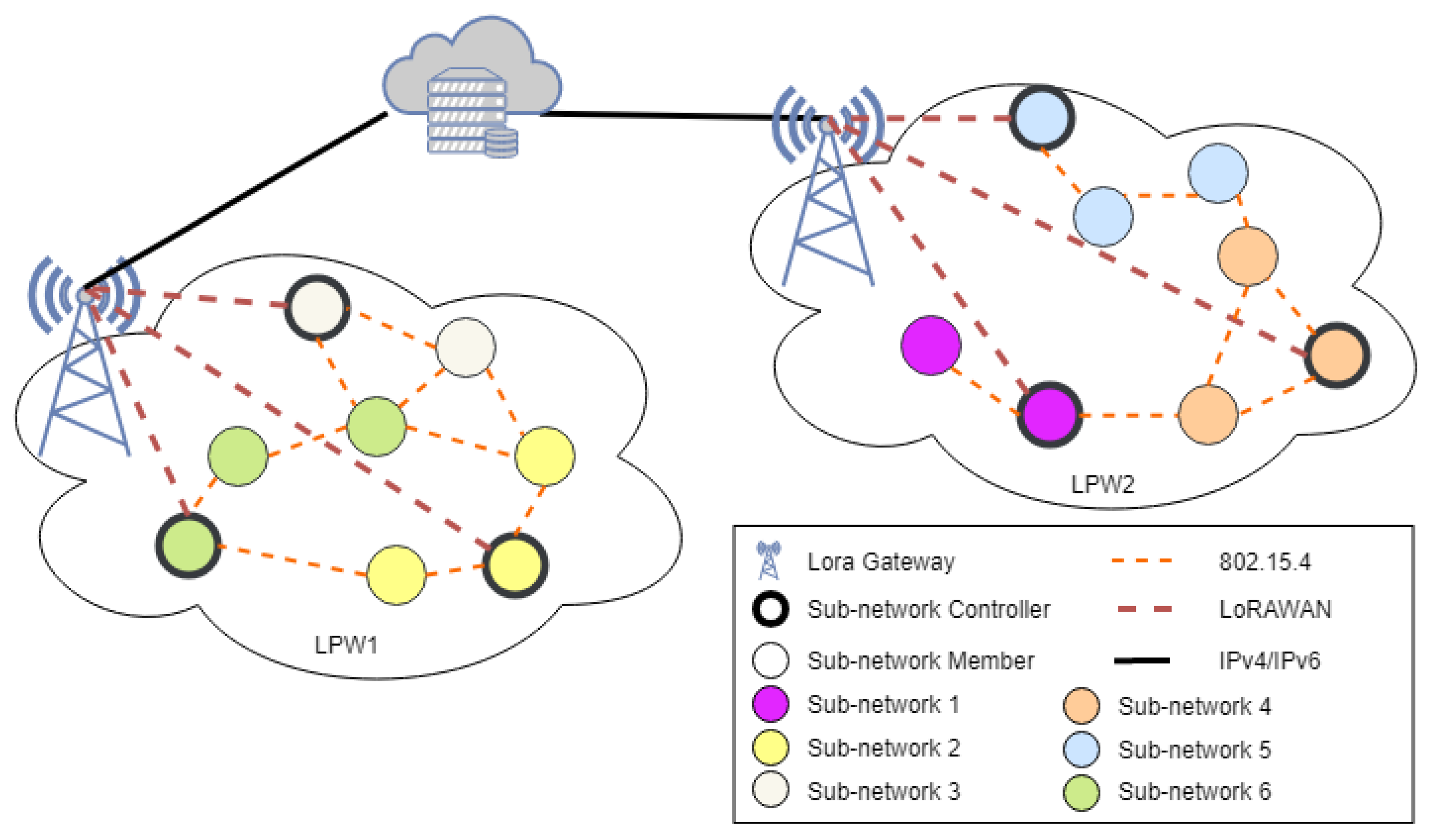
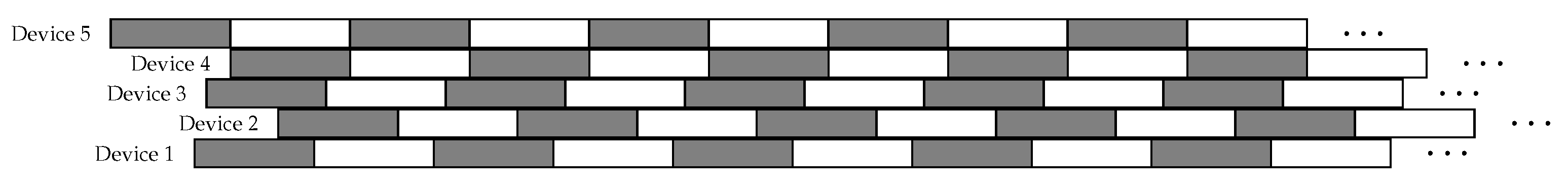
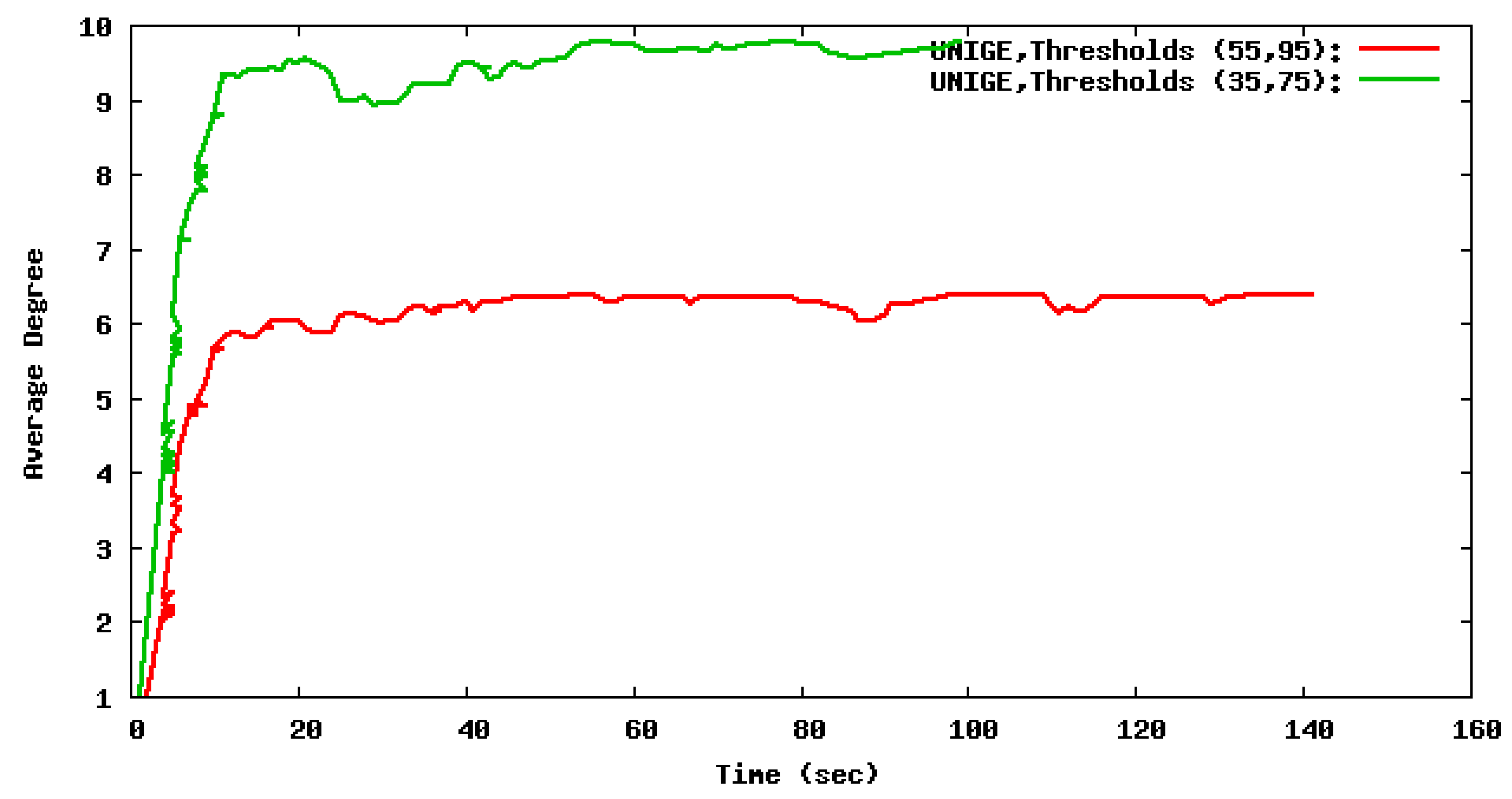
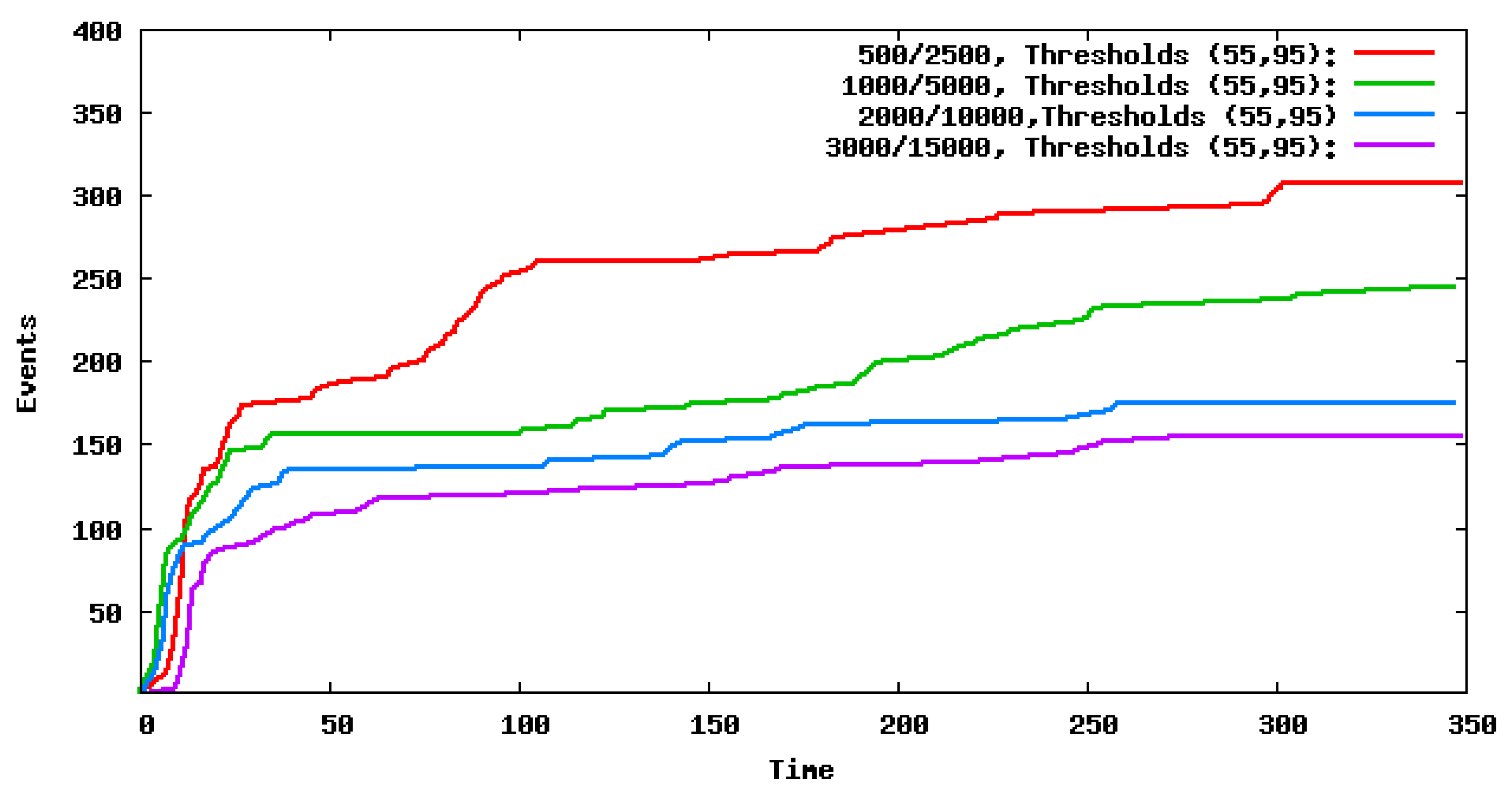
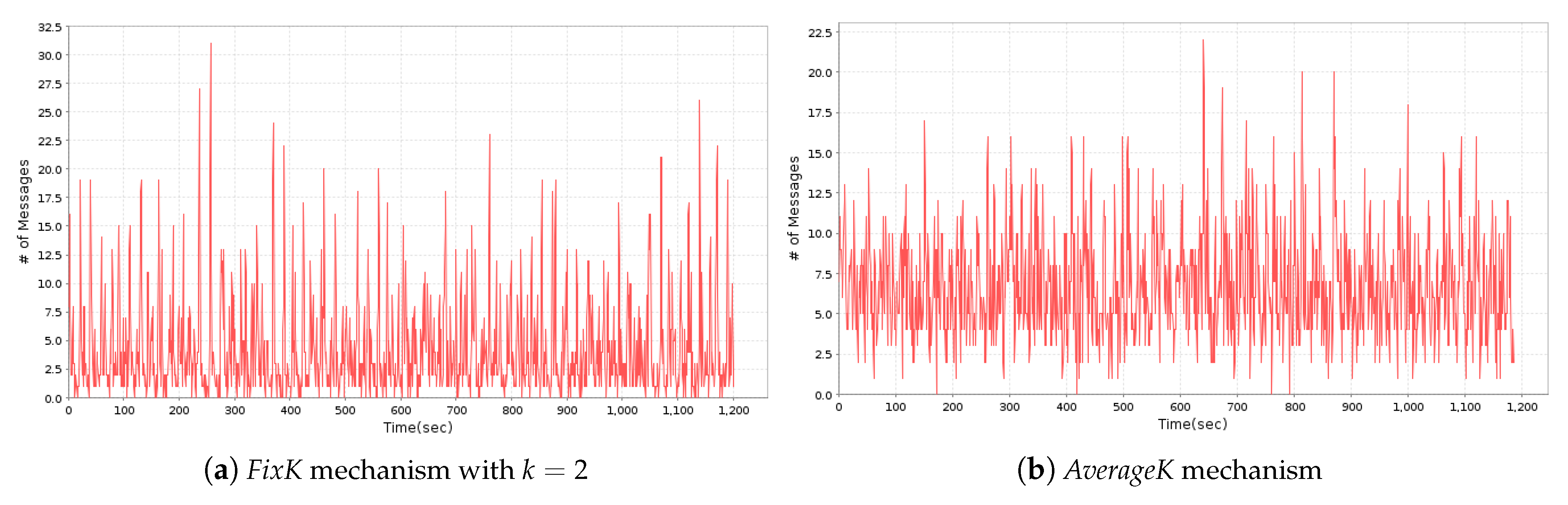
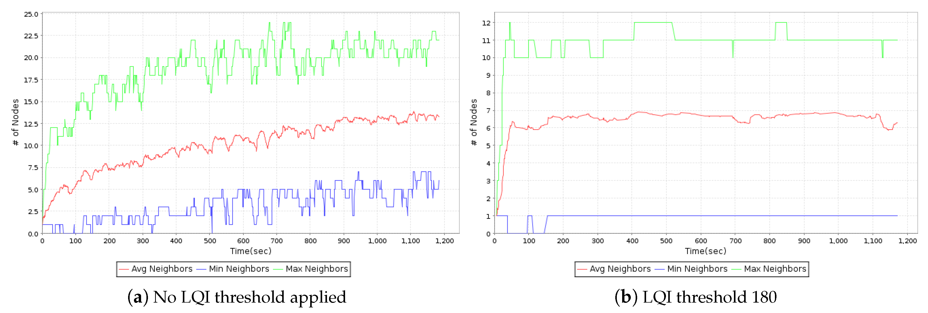
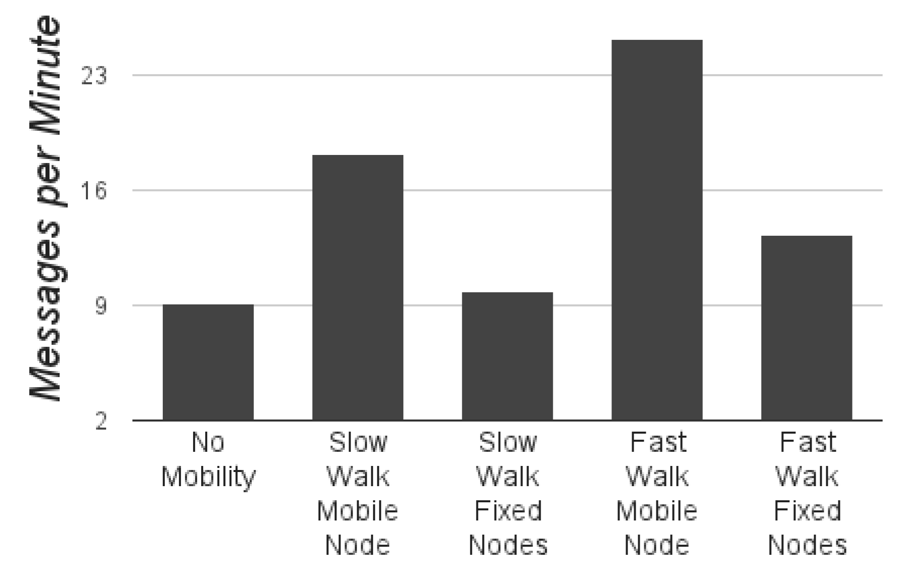
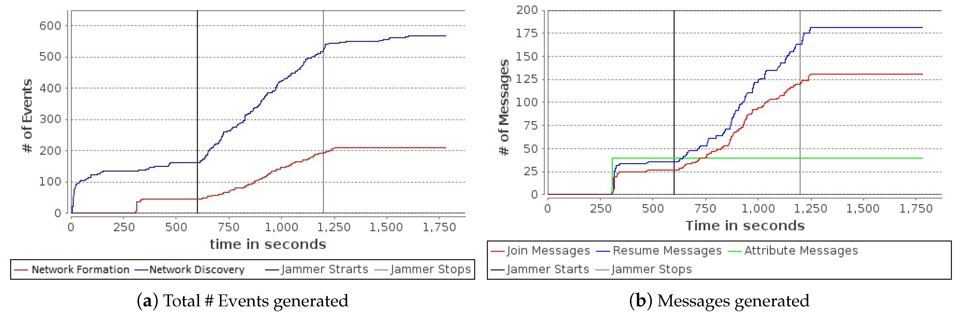
Table 1.
Network lifetime during sub-network detection.
| DC | Lifetime | Extension |
|---|---|---|
| 100% | 1709 min | - |
| 80% | 1861 min | 8.9% |
| 70% | 2035 min | 19% |
| 50% | 3222 min | 88.5% |
| 30% | 4662 min | 172% |
© 2018 by the authors. Licensee MDPI, Basel, Switzerland. This article is an open access article distributed under the terms and conditions of the Creative Commons Attribution (CC BY) license (http://creativecommons.org/licenses/by/4.0/).
Share and Cite
MDPI and ACS Style
Amaxilatis, D.; Chatzigiannakis, I. Design and Analysis of Adaptive Hierarchical Low-Power Long-Range Networks. J. Sens. Actuator Netw. 2018, 7, 51. https://doi.org/10.3390/jsan7040051
AMA Style
Amaxilatis D, Chatzigiannakis I. Design and Analysis of Adaptive Hierarchical Low-Power Long-Range Networks. Journal of Sensor and Actuator Networks. 2018; 7(4):51. https://doi.org/10.3390/jsan7040051
Chicago/Turabian StyleAmaxilatis, Dimitrios, and Ioannis Chatzigiannakis. 2018. "Design and Analysis of Adaptive Hierarchical Low-Power Long-Range Networks" Journal of Sensor and Actuator Networks 7, no. 4: 51. https://doi.org/10.3390/jsan7040051
Note that from the first issue of 2016, this journal uses article numbers instead of page numbers. See further details here.