Structural Compressed Panel VAR with Stochastic Volatility: A Robust Bayesian Model Averaging Procedure

Abstract

This paper improves the existing literature on the shrinkage of high dimensional model and parameter spaces through Bayesian priors and Markov Chains algorithms. A hierarchical semiparametric Bayes approach is developed to overtake limits and misspecificity involved in compressed regression models. Methodologically, a multicountry large structural Panel Vector Autoregression is compressed through a robust model averaging to select the best subset across all possible combinations of predictors, where robust stands for the use of mixtures of proper conjugate priors. Concerning dynamic analysis, volatility changes and conditional density forecasts are addressed ensuring accurate predictive performance and capability. An empirical and simulated experiment are developed to highlight and discuss the functioning of the estimating procedure and forecasting accuracy.

1. Introduction

This study aims to construct and develop a methodology to improve the Bayesian compressed regression literature when dealing with (i) time-varying parameters, (ii) volatility changes, (iii) the curse of dimensionality, and (iv) variable selection problems accounting for large model and parameter spaces.

In macroeconomics and finance, existing approaches involve estimating high dimensional multicountry Vector Autoregressions (VARs) and Panel VARs (PVARs) to appropriately model and evaluate time-varying linkages among sectors and countries, where the number of parameters are highly larger than the obervational data. In thix context, prior specification strategies and Monte Carlo Markov Chain (MCMC) algorithms are constructed according to past information on the parameters’ distributions in order to transform overparameterized models in low-dimensional parameter space. In this way, forecasting analysis and policy evaluations are feasible and can be performed ensuring good accuracy and quality of the point estimates. Most studies based on this literature focus on frequentist and Bayesian approaches. The former generally work with a sparse hierarchical prior distribution allowing to discriminate between zero and non-zero factor loadings in order to identify unobserved factors and then provide a meaningful economic interpretation for them. See, among many other, Bernanke et al. (2005) (Factor-Augmented VARs); Pesaran et al. (2009) and Pesaran et al. (2004) (multicountry Dynamic Factor Models); Dees et al. (2007); Feldkircher and Huber (2016); Cuaresma et al. (2016); Dovern et al. (2016); and Huber (2016) (Global VARs); and Cogley et al. (2005); Primiceri (2005); Koop and Korobilis (2009); Canova and Forero (2015); Banbura et al. (2010); and Koop and Korobilis (2013) (Time-Varying Parameter VARs with multivariate stochastic volatility). Conversely, according to Bayesian models, they typically use diffuse or informative priors to shrinkage high-dimensional parameter spaces relying on computationally intensive MCMC algorithms in order to perform recursive forecasting exercises (see, for instance, Canova and Ciccarelli (2009); Koop and Korobilis (2016); Giannone et al. (2015); Carriero et al. (2015a, 2016); Koop (2013); Korobilis (2016); George et al. (2008); Carriero et al. (2009); Canova and Ciccarelli (2016); Canova and Forero (2015); Pacifico (2019, 2021)). Nevertheless, these methods requiring the use of MCMC algorithms and implementations are still not suitable for forecasting with thousands of variables, that would be possible with random compression.

Concerning related Bayesian dimensionality reduction approaches, Bayesian compressed regression models have been also used in macroeconomics, where high dimensional parameter spaces are compressed by randomly drawing different projections according to the explanatory variables (see, for instance, Guhaniyogi and Dunson (2015) among others). They refer to supervised data compression method involving the use of Bayesian Model Averaging (BMA) to assign different weights to the drawn projections based on the explanatory power of the compressed covariates. However, the compressed regression does not include any reference to the variable(s) of interest and then can result in inaccurate estimates when the data show highly large causal relationships. In addition, the data compression involved in these methods are unable to deal with variable selection problems such as model uncertainty when a single model is selected a priori to be the true one (see, e.g., Madigan and Raftery (1994); Madigan et al. (1995); Raftery et al. (1995, 1997)), endogeneity issues due to unobserved heterogeneity and omitted factors (see, for instance, Gelfand and Dey (1994) and Pacifico (2020b) for related works), and risk of overfitting occurring when the model is too rich relative to the sample size (see, for instance, Mullainathan and Spiess (2017) and Pacifico (2020b) for more discussion).

As opposed to these models, Bayesian Compressed VARs (BCVARs) cover an important role as an alternative to variable selection or shrinkage in high dimensional settings, by randomly compressing the predictors prior to analysis. In this context, the curse of dimensionality affecting the estimating process performance is minimized, obtaining a low-dimensional subset of the predictors better fitting the data with minimal loss of information about their response (explanatory power) for the dependent variable(s). The prior specification strategy is more flexible—requiring less restrictive features—and the exact posterior distribution conditional on the compressed data is available analytically, resulting in shrinkage of high dimensional model and parameter spaces. Model averaging is used to reduce sensitivity to the random projection matrix, while accommodating uncertainty in the subspace dimension. In this way, BCVARs entail less computational costs by increasing the speed at which the dependent variable(s) return to equilibrium after a change in the subset of potential predictors and bypassing robustness issues due to convergence and mixing problems with intensive MCMC methods. Thus, recursive forecasting methods become computationally feasible for policy-making (see, for instance, Taveeapiradeecharoen and Aunsri (2020); Taveeapiradeecharoen et al. (2019); and Götz and Haustein (2018) for some important tools in macroeconomics and finance). However, in macroeconomic forecasting applications, ignoring volatility changes (because of structural changes and policy regime shifts) and time-variation in the coefficients and/or error covariance matrix, the estimation procedure results in bad (or biased) estimates and poor (or low) quality of density forecasts (see, for instance, Jacquier et al. (1994); Carriero et al. (2015b, 2019); Clark (2011); Cogley and Sargent (2005); Primiceri (2005); and D’Agostino et al. (2013) (stochastic volatility and structural changes); and Clark and Ravazzolo (2015) and Pacifico (2021) (time-varying volatility)).

Recently, Koop et al. (2019) developed a BCVAR with time-varying parameters and stochastic volatility by extending the Guhaniyogi and Dunson (2015)’s Bayesian random compression method. More precisely, the two main features introduced are: (i) the extension to the VAR case using a BMA to obtain the subset of the VAR coefficients better explaining the dependent variable(s) and the parameters better describing volatility purposes, and (ii) a random process to shrink the large VAR in a low-dimensional subspace of predictors according to the explanatory power they have for the dependent variable(s). A macroeconomic application highlights the estimating process performance and forecasting accuracy using an univariate Autoregressive process with a single lagged term (AR(1)) as benchmark approach. Compared with the previous models, their method fits better the data and achieve more accurate forecasts. However, the BMA used in shrinkage of high dimensional parameter spaces consists in assigning different weights to the projections based on the explanatory power of the predictors rather than the model size. Thus, open variable selection issues when dealing with overparameterization—such as model misspecification problems and overfitting—are not addressed. In addition, the number of different projections are generated randomly and then does not involve the data. Even if it is computationally useful in multiple model classes, common parameters can change meaning from one model to another, so that prior distributions should change in a corresponding fashion and be weighted more according to the model size. Last but not least, when studying macroeconomic–financial linkages, issues concerning heterogeneity, interdependence, and commonality among countries and sectors should be accounted for.

My computational approach aims to overtake these limits when estimating Bayesian compressed regressions in large VAR settings with time-varying parameters and multivariate stochastic volatilities. More precisely, its implementation consists of combining and extending the underlying logic in Pacifico (2020b), regarding variable selection problems in multiple model classes, and in Pacifico (2021), concerning high dimensional multicountry dynamic analysis. Thus, conversely to Koop et al. (2019), the main features are: (i) the selection of the best subset of predictors through Posterior Model Probabilities rather random draws in order to weight priors according to the model size; and (ii) the estimation of a structural panel framework when jointly modelling parameter and model spaces in order to perform accurate cross-country forecasts and policy issues. Here, best stands stands for the model providing the most accurate predictive performance over all candidate models, and PMP denots the probability of each candidate model fitting the data. Methodologically, the developed approach—named Structural Bayesian Compressed PVAR (SBCPVAR) model—is based on semiparametric prior assumptions to entail a strong model selection in high dimensional model classes and MCMC algorithms to construct posterior distributions.

In detail, the contributions of the proposed methodology are fourfold. First, additional data matrices are considered containing predetermined1 variables (e.g., lagged dependent and control variables) and observable endogenous variables including macroeconomic–financial and socioeconomic–demographic factors. Multivariate Conjugate Informative Proper Mixture (mvCIPM) priors and MCMC-based PMPs are then used in oder to: (i) include all the information from the whole multidimensional framework; (ii) impose specification choices to compress high dimensional parameter and model spaces; and (iii) jointly deal with variable selection problems (model uncertainty and overfitting), endogeneity issues, and structural model uncertainty (because of one or more parameters are posited as the source of model misspecification problems). The mvCIPM priors are an implementation of the conjugate informative proper priors in Pacifico (2020b) to deal with overparameterization in large time-varying PVAR.

Second, related to the previous feature, properly specification choices to drop or down-weight bad compressions are addressed instead of compressing the data randomly. To do it, I build on and extend the Pacifico (2020b)’s analysis, who develops a Robust Open Bayesian (ROB) procedure in two stages for implementing BMA and BMS in multiple linear regression models and time-varying high dimensional multivariate data when studying cross-country dynamic economics. In this way, the best subset of model solutions is obtained by defining a criterion in accordance with either the data (explanatory power) and the model size (different interactions between covariates). Thus, the complete compressed subset regression method uses model-weighted combinations of all available subsets of predictors and resorts to a less restrictive supervised dimension reduction technique. However, that framework even if ensures better accuracy and quality of the density forecasts, it would highly increase the computational costs involved in the procedure, representing an important limit to be dealt with.

Third, I adapt the Pacifico (2021)’s strategy to transform an overparameterized structural PVAR into a compressed Seemingly Unrelated Regression model in order to account for interdependence, heterogeneity (or homogeneity), and commonality when studying macroeconomic–financial linkages. More precisely, I involve some auxiliary regression parameters in the extended ROB procedure to evaluate the time-varying VAR coefficients for each country-variable pair in presence of potential unobserved changes (volatility effects). Then, I construct a flexible factorization for the compressed regression parameters to make them estimable. Finally, a multivariate Bayesian Information Criterion (mvBIC) is used to depict the optimal number of lags in high dimensional multivariate model selection, extending the standard BIC to the case of multiple response variables (see, for instance, Sofer et al. (2014)).

Fourth, MCMC algorithms are addressed to construct appropriate posterior distributions and then perform cross-country conditional density forecasts. The diagnostic measure computed to measure forecasting accuracy and then account for relative regrets dealing with semiparametric forecasting problem is the multivariate Weighted Mean Squared Forecast Error of Christoffersen and Diebold (1998).

An empirical application involving more than hundreds of macroeconomic–financial and socioeconomic–demographic variables is developed to highlight the performance of the proposed methodology. The empirical strategy is able to design conditional density forecasts and strategic policy measures investigating either the impact of COVID-19 pandemic or real/financial shocks on potential output in a pool of advanced and emerging countries, with ’potential output’ denoting the highest level of economic activity. Furthermore, a simulated experiment—compared to related works—is also addressed to discuss theoretical properties.

The remainder of this paper is organized as follows. Section 2 introduces the econometric framework and the estimating method. Section 3 displays the Bayesian model selection procedure by clarifying prior specification strategy and posterior distributions. Section 4 describes the data and the empirical analysis. Section 5 provides a simulated example through Monte Carlo simulations to discuss theoretical properties and forecasting accuracy compared to some existing approaches. The final section contains some concluding remarks.

2. Econometric Model

2.1. Model Estimation

Consider a simplified version of the multicountry SPBVAR model developed in Pacifico (2021):

$$Y_{im,t}=\sum _{\lambda =1}^l\left[A_{im,j\tilde{m}}{Y}_{im,t-\lambda }+B_{i\xi ,j\tilde{\xi }}{Z}_{i\xi ,t-\lambda }\right]+{\epsilon }_{im,t},$$

(1)

where the subscripts $(i,j)=1,2,\dots ,N$ are country indices, $t=1,2,\dots ,T$ denotes time, $m=1,2,\dots ,M$ and $\xi =1,2,\dots ,\Xi$ are directly observed endogenous variables for i, with $\tilde{m}=1,2,\dots ,\tilde{M}$ and $\tilde{\xi }=1,2,\dots ,\tilde{\Xi }$ referring to the ones observed for j and independent of i, $\lambda =1,2,\dots ,l$ stands for all available lags of every time-varying variable to be potentially included in the shrinking process, and ${\epsilon }_{im,t}\sim i.i.d.N(0,{\Omega }_t)$ is an $NM·1$ vector of heteroscedastic unobservable shocks with variance-covariance matrix ${\Omega }_t$.

Stacking for $(m,\xi ,\tilde{m},\tilde{\xi })$, all terms within the system are so defined. (i) $Y_{i,t}$ is an $NM·1$ vector of observed variables to be predicted for each i for a given m. (ii) $A_{i,j}$ are $NM\times NM$ matrices of lagged coefficients for each pair of countries $(i,j)$ for a given m, and $Y_{i,t-\lambda }$ is an $NM·1$ vector of observed lagged variables for each i for a given m. In this study, I decompose it in $Y_{i,t-\lambda }={\left[Y_{i,t-\lambda }^{o^{\prime }},Y_{i,t-\lambda }^{c^{\prime }}\right]}^{{}^{\prime }}$, with $Y_{i,t-\lambda }^{o^{\prime }}$ denoting lagged outcomes (e.g., country’s productivity) to capture the persistence and $Y_{i,t-\lambda }^{c^{\prime }}$ including lagged control variables such as general economic–financial conditions. (iii) $B_{i,j}$ are $N\Xi \times N\Xi$ matrices of lagged coefficients for each pair of countries $(i,j)$ for a given $\xi$, and $Z_{i,t-\lambda }$ is an $N\Xi ·1$ vector including a set of additional observed lagged endogenous factors for each i for a given $\xi$. Let the model (1) be a VAR process, when performing forecasting analysis, every outcome for each country would depend on its lagged values ($Y_{it-\lambda }^{o^{\prime }}$) and sudden changes in $Y_{it-\lambda }^{c^{\prime }}$ due to unexpected shocks (misspecified dynamics). However, when studying macroeconomic–financial linkages, other potentially endogenous related factors would affect outcomes’ distribution because of not directly observed/measured relationships (endogenity issues). In this study, I evaluate them assuming the decomposition $Z_{i,t-\lambda }={\left[Z_{i,t-\lambda }^{s^{\prime }},Z_{i,t-\lambda }^{p^{\prime }}\right]}^{{}^{\prime }}$ referring to socioeconomic–demographic conditions and policy factors, respectively. Then, in order to perform a Bayesian compressed variable selection regression, I model the framework combining the (non-)homogeneous parameters into a $1·Nk$ vector $X_t={(Y_{im,t-1}^{{}^{\prime }},Y_{im,t-2}^{{}^{\prime }},\dots ,Y_{im,t-l}^{{}^{\prime }},Z_{i\xi ,t-1}^{{}^{\prime }},Z_{i\xi ,t-2}^{{}^{\prime }},\dots ,Z_{i\xi ,t-l}^{{}^{\prime }})}^{{}^{\prime }}$ and construct an auxiliary parameter ${\Theta }_t$—indexed k—grouping the two matrices of time-varying coefficients, where $k=[M+\Xi ]·l$ corresponds to the number of all matrix coefficients in each equation of model (1) for each pair of countries $(i,j)$. Thus, the parameter ${\Theta }_t=(A_{im,j1},A_{im,j2},\dots ,A_{im,j\tilde{M}},B_{i\xi ,j1},B_{i\xi ,j2},\dots ,B_{i\xi ,j\tilde{\Xi }})$ looks like a set of matrices of size $NM\times Nk$. Nevertheless, with these specifications, the (1) faces to be unfeasible and unreliable because of (possible) different dimensions between matrices ($A_{i,j},B_{i,j}$) and high dimensional parameter spaces, respectively. The proposed methodology overcomes these problems by using a hierarchical factor structure and a prior shrinkage based on a multivariate ROB (mvROB) procedure.

For notational simplicity, I display the estimating procedure with no deterministic terms2. The heteroscedasticity imposed in the variance-covariance matrix of the vector of innovations (${\epsilon }_{i,t}$) is to capture and then investigate potential unobserved shocks (impulse) among variables affecting cross-country spillover effects on the outcomes (response). It is worth noting that when studying macroeconomic–financial linkages and other related socioeconomic–demographic effects, the model in (1) is going to admit multiple and multivariate structural breaks and policy regime shifts. Thus, according to the Primiceri (2005)’s modelling strategy, without loss of generality, I re-write the error terms in (1) as:

$${\epsilon }_{i,t}={\Delta }_t·{\omega }_{i,t}\mathrm{with}{\Omega }_t={\Delta }_t{\Delta }_t^{{}^{\prime }},$$

(2)

where ${\Delta }_t$ is an $NM\times Nk$ matrix with elements either potentially different from zero or close to zero and ${\omega }_{i,t}\sim N(0,I_{Nk})$ is a $Nk·1$ vector for each set of variables $(m,\xi )$. As an illustrative example, stacking for m and k for simplicity, consider the following structure for ${\Delta }_t$, in a three-by-three case:

$${\Delta }_t=\underset{(3\times 3)}{\left(\begin{array}{ccc}{d}_{i,j}& 0& d_{i,j}\\ d_{i,j}& d_{i,j}& d_{i,j}\\ d_{i,j}& 0& d_{i,j}\end{array}\right)},$$

(3)

where the $d_{i,j}$’s indicate the elements potentially different from zero. Equation (3) implies a variance covariance matrix of the residuals with zero in the positions ($1,2$) and ($3,2$). In case of triangular decomposition, the solution would be incompatible with draws of ${\Omega }_t$ or at least approximate whether the elements ($1,2$) and ($3,2$) are very close to zero. However, the latter does not ensure efficient estimation in a context of overidentified systems, unless the overidentification derives from further zero restrictions. In addition, when studying time-varying linkages, time-invariant variance-covariance matrices are undesirable or too restrictive.

In this study, a more flexible Bayesian inference is addressed in order to overtake these model misspecification problems by taking advantage of the shrinking process involved in the procedure. More precisely, two considerations are in order: the use of a random walk process to easily model the time-varying distributions of the elements in ${\Delta }_t$ and a compression regression form to evaluate the time-varying coefficient vectors for each country–variable pair (${\Theta }_t$) in presence of unobserved changes ($d_{i,j}\ne 0$).

Let ${\delta }_t=vec\left({\Delta }_t\right)=vec{(d_{im,j1}^{{}^{\prime }},d_{im,j2}^{{}^{\prime }},\dots ,d_{im,j\overline{k}}^{{}^{\prime }})}^{{}^{\prime }}$ be a $NMK·1$ vector containing—stacked by columns—the elements of the matrix ${\Delta }_t$, with $K=Nk$ and $\overline{k}$ denoting the maximum value of the time-varying VAR coefficients for each pair of countries $(i,j)$, the parameter ${\delta }_t$ is then modelled as a random walk process:

$${\delta }_t={\delta }_{t-1}+v_t\mathtt{with}{v}_t\sim N(0,{\Sigma }_{\delta }),$$

(4)

where ${\Sigma }_{\delta }=diag({\sigma }_{d_{im,j1}}^2,{\sigma }_{d_{im,j2}}^2,\dots ,{\sigma }_{d_{im,j\overline{k}}}^2)$ is a block diagonal covariance matrix of size $NM\times NM$ defined according to the time-varying vector ${\delta }_t$ for each pair of countries $(i,j)$, and ${\delta }_0$ denotes the initial conditions to be estimated. Here, the variances generated by (4) are unobserved components treated as permament shifts. I recall that random-walk assumption assumed in (4) is an useful way to easily model time-varying parameters when studying high dimensional multivariate dynamic models for a finite period of time. Thus, one is able to: (i) reduce the number of parameters; (ii) allow for the evaluation of permanent shifts; (iii) investigate any type of coefficient factors via their interactions; and (iv) replace volatility changes by coefficient changes.

Here, some considerations are in order. (i) As discussed in Primiceri (2005), according to some residuals’ positions, elements in ${\Delta }_t$ different from or very close to zero would lead to the solution to be approximate (even if probably still reliable) or rejected, respectively. This limit is overtaken in this study by means of the variable selection procedure involved in the empirical strategy. More precisely, the vector ${\delta }_t$ accounts for unobserved changes when studying k time-varying variables’ distributions and their interactions (cross-terms). Thus, whether a model solution (or combination of predictors $X_t$) is likely reliable, the BMS used in the ROB procedure would automatically discard it by the data. Indeed, whether a model solution is rejected, it means that no change-points (or structural breaks) and policy regime shifts matter. In macroeconomics and finance, when investigating international spillover effects given unexpected shocks, that scenario is implausible or—on the contrary—a signal of an unfounded empirical case-study. (ii) In (2), the identification I use is not based on a triangular decomposition of ${\Omega }_t$ as with Koop et al. (2019) and Carriero et al. (2015b), requiring an additional triangular scheme on ${\Delta }_t$. Conversely, the identifiability of ${\delta }_t$’s is guaranteed from the block diagonality of ${\Sigma }_{\delta }$. The idea is to absorb potential excessive spillover effects in the parameter ${\Theta }_t$ whether they matter (${\delta }_t\ne 0$) or discarding them otherwise (${\delta }_t\simeq 0$), where excessive stands for a sudden (not directly observed) highly large intensification of the spreading of spillovers among countries and/or sectors. Thus, such a specification implies that volatility changes due to the presence of unobserved components are replaced by coefficient changes and dealt with parameter shifts. (iii) In this study, potential volatility changes are investigated through the excess kurtosis (${\kappa }_{i,t}$) of the SPBVAR prediction error evaluated over the information on the past year (${\mathfrak{F}}_{-1}$). As highlighted in Koop et al. (2019) according to the GARCH literature, let the error terms be Normally distributed, the excess kurtosis will be high in times of large volatility and zero otherwise. (iv) According to the previous point, the empirical procedure would tend to be sufficiently restrictive evaluating multiple structural breaks through permanent shifts. A possible extension could be—for example—assuming time-varying log-volatilities in (1), just as in Pacifico (2021). In that context, Autoregressive Conditional Heteroskedasticity in Mean model effects are used to model time-varying conditional second moments so as to quantify unexpected variations in $Y_t$. The variance-covariance matrix of the vector of innovations (${\Omega }_t$) would be then a diagonal matrix containing the time-varying log-volatilities ${\delta }_t={({\delta }_{1t},{\delta }_{2t},\dots ,{\delta }_{Nt})}^{{}^{\prime }}$. Even if it improves the performance of conditional density forecasts, highly larger computational costs matter requiring the use of MCMC implementations (such as Metropolis-Hastings algorithm). (v) Potential structural changes, dynamic feedback, and interactions among countries and variables are possible and allowed to vary over time. Thus, the framework of (1) makes it able to investigate and quantify international business cycles, policy implications, and economic dynamics by jointly dealing with endogeneity and volatility changes and functional forms of misspecification. These features are then able to perform accurate conditional density forecasts. (vi) Finally, the framework can be related to the literature on cointegrating approaches with time-varying coefficients. More precisely, they provide an efficient method of estimation to model macroeconomic–financial long-run relationships, where the coefficients are estimated nonparametrically as smooth functions evolving over time (see, among many other, Hansen (1992); Quintos and Phillips (1993); and Andrews (1991a, 1991b)). However, this study does not rely on these methods because of their fruitless in multicountry dynamic analyses due to the presence of omitted variables or parameter instability (e.g., endogeneity issues) and unobserved change-points (e.g., misspecified dynamics).

With these specifications, I re-write (1) expressing it in a simultaneous-equation form:

$$Y_t={\Theta }_t{X}_t^{{}^{\prime }}+{\Delta }_t{\omega }_{i,t},$$

(5)

where $Y_t={(Y_{1m,t}^{{}^{\prime }},\dots ,Y_{Nm,t}^{{}^{\prime }})}^{{}^{\prime }}$ is an $NM·1$ vector containing the observable variables of interest and $X_t^{{}^{\prime }}$ is a $Nk·1$ vector.

Let ${\Gamma }_t=({\Theta }_t,{\Delta }_t)=(A_{im,j1},{\Delta }_t,A_{im,j2},{\Delta }_t,\dots ,A_{im,j\tilde{M}},{\Delta }_t,B_{i\xi ,j1},{\Delta }_t,B_{i\xi ,j2},{\Delta }_t,\dots ,$

$B_{i\xi ,j\tilde{\Xi }},{\Delta }_t)$ be a $NM\times Nk$ matrices where every coefficient matrix ($A_{i,t},B_{i,j}$) is combined with the time-varying (unobserved) elements of ${\Delta }_t$, and ${\gamma }_t=vec\left({\Gamma }_t\right)$ be a $NMK·1$ vector containing—stacked into a vector—the time-varying coefficient vectors for each country–variable pair. More precisely, the idea is to evaluate cross-unit lagged interdependencies and dynamic feedback dealing with potential unobserved changes (volatility effects). Thus, in times of large volatility (${\delta }_t\ne 0$), the construction of ${\Gamma }_t$ would absorb and then include these unexpected shocks in the estimating procedure.

The reduced form in (5) can be re-written according to a compression regression form:

$$Y_t={\Gamma }_t\left(X_t^{{}^{\prime }}+{\omega }_{i,t}\right).$$

The variable selection problem arises when there is some unknown subset of $X_t$ with predictors so small that it would be preferable to ignore them. Thus, the variable selection procedure can be seen as one of deciding which of the ${\gamma }_t$’s regression parameters are sufficiently small so that the predictor $X_t$ should be ruled out from the system. Its aim is to evaluate $2^K$ subset choices, referring to any potential model solution (or combination of predictors $X_t$) better fitting the data. Now, because the coefficient vectors in ${\gamma }_t$ vary in different time periods for each country–variable pair and there are more coefficients than data points, it is impossible to evaluate them. To solve these problems, I apply a flexible factorization for ${\gamma }_t$ to estimate all coefficients and their possible interactions without restrictions or loss of efficiency. The curse of dimensionality is then dealt with performing the mvROB procedure in order to select the only ${\gamma }_t$’s regression parameters sufficiently large to be included in the system.

Let ${\varphi }_t$ be an additional auxiliary parameter containing the compressed ${\gamma }_t$’s regression parameters (${\gamma }_t^c$), I assume the following factor structure:

$${\gamma }_t^c={\Phi }_t·{\varphi }_t+u_t,$$

(6)

where ${\varphi }_t$ denotes a $N\phi ·1$, with $N\phi \ll NMK$ and $\{1\le \phi <k\}$, $dim\left({\varphi }_t\right)\ll dim\left({\gamma }_t\right)$ by construction, ${\gamma }_t^c$ refers to the compressed time-varying coefficient vectors obtained through the shrinking process, ${\Phi }_t$ is a $NMK\times N\phi$ conformable matrix with elements equal to zero (${\gamma }_t^c$ small and then absence of k-th covariate in the model for a given i) and one (${\gamma }_t^c$ sufficiently large and then presence of k-th covariate in the model for a given i), and $u_t$ is a $NMK·1$ vector of disturbances with zero mean and variance-covariance matrix ${\Sigma }_u$, with ${\Sigma }_u=V·{\sigma }_t$, with $V={\sigma }^2·I_{NMK}$ as in Kadiyala and Karlsson (1997) according to the methodology and ${\sigma }_t\cong {\Omega }_t\otimes \left(X_t^{{}^{\prime }}{X}_t\right)$ denoting (potential) volatility changes. In this study, the auxiliary variable ${\varphi }_t$ is supposed to follow a random walk process:

$${\varphi }_t={\varphi }_{t-1}+{\eta }_t\mathrm{with}{\eta }_t\sim N(0,{\Psi }_t),$$

(7)

where ${\Psi }_t=diag({\Psi }_{mt,1},{\Psi }_{mt,2},\dots ,{\Psi }_{mt,\overline{k}})$ is a block diagonal matrix, and ${\Psi }_{mt,k}=({\psi }_t\times I_{NMK})$, with ${\psi }_t$ controlling the stringent conditions of the shrinking process of the time-varying compressed coefficient parameters (${\gamma }_t^c$) in order to make them estimable. Here, $u_t$ and ${\psi }_t$ are correlated between them by construction, and ${\eta }_t$ and ${\psi }_t$ are allowed to be correlated between them.

According to the factorization in Equation (6) and let ${\tilde{X}}_t=I_{NM}\otimes (X_t+{\omega }_{i,t}^{{}^{\prime }})$ be an $NM\times NMK$ matrix containing all lagged time-varying variables and volatility elements within the system stacked in $X_t$ and ${\omega }_{i,t}$ (respectively), the reduced-form SPBVAR model in Equation (5) can be transformed into a Compressed Seemingly Unrelated Regression (CSUR) model:

$$Y_t={\tilde{X}}_t\left[\left({\Phi }_t·{\varphi }_t\right)+u_t\right]\equiv {\chi }_t^c{\varphi }_t+E_t^c,$$

(8)

where ${\chi }_t^c\equiv ({\tilde{X}}_t·{\Phi }_t)$ are $NM\times N\phi$ matrices that stack all coefficients and their possible interactions in the multicountry SPBVAR model in (1), and $E_t^c\equiv {\tilde{X}}_t·u_t$ is an $NM·1$ vector having a particular heteroskedastic covariance matrix that needs to be accounted for.

2.2. Multivariate ROB Procedure

Let $M_K=(M_{i1},M_{i2},\dots ,M_{i\overline{k}})$ be a countable collection of all $2^K$ possible subset choices, with $\overline{k}$ denoting the maximum value of the time-varying matrix coefficients in (1). The full model class set is:

$$\mathcal{F}=\left\{M_K:M_K\subset \mathcal{F},M_K\in \mathcal{M},k\in \mathcal{K},{\Theta }_t{X}_t^{{}^{\prime }}+{\Delta }_t{\omega }_t\right\},$$

where $\mathcal{M}$ and $\mathcal{K}$ denote the multidimensional natural model and parameter spaces, respectively.

According to the Pacifico (2020b)’s framework, I match all (potential) candidate models to shrink both the model space ($\mathcal{M}$) and the parameter space ($\mathcal{K}$). The shrinkage jointly deals with overestimation of effect sizes (or individual combinations), dynamic interactions (or cross-term lagged interdependencies), model uncertainty and misspecification problems (implicit in the procedure), and endogeneity and volatility changes (involved in the hierarchical framework).

Let the PMPs denote the probability of each candidate model fitting the data, they can be defined as:

$$\pi \left(M_K\right|Y_t)=\frac{\pi \left(Y_t\right|M_K)·\pi \left(M_K\right)}{{\sum }_{M_K\in \mathcal{M}}\pi \left(Y_t\right|M_K)·\pi \left(M_K\right)},$$

(9)

where $\pi \left(Y_t\right|M_K)=\int \pi \left(Y_t\right|M_K,{\gamma }_t)·\pi \left({\gamma }_t\right|M_K)d{\gamma }_t$ is the marginal likelihood, and $\pi \left({\gamma }_t\right|M_K)$ is the conditional prior distribution of ${\gamma }_t$ given $M_K$. However, when N is high dimensional and T sufficiently large, the calculation of the integral $\pi \left(Y_t\right|M_K)$ is unfeasible and then MCMC methods and implementations are needed.

The mvROB procedure entails in jointly shrinking the model $\mathcal{M}$ and the parameter $\mathcal{K}$ space to make Equation (9) estimable. Then, a lower-dimensional model class set is obtained containing the only best model solutions (or combinations of predictors) fitting the data. It corresponds to:

$$\mathcal{E}=\left\{M_F:M_F\subset \mathcal{E},\mathcal{E}\subset \mathcal{F},\sum _{M_K\in \mathcal{M}}\pi \left(M_F\right|Y_t,{\varphi }_t)\ge \tau \right\},$$

where $M_F$ denotes the submodel solutions of the CSUR in (8), with $M_F<M_K$, $F\ll K$, where $F=N\phi$ and $\{1\le \phi <k\}$, and $\tau$ is a threshold chosen arbitrarily for an enough posterior consistency3. In this study, I use $\tau =5\%$ with N high dimensional and then more restrictive than the one used in Pacifico (2020b).

The final model solution to perform forecasting and policy-making corresponds to one of the submodels $M_F$ with higher log natural Bayes Factor (lBF):

$$lB{F}_{\phi ,k}=log\left\{\frac{\pi \left(M_F\right|Y_t)}{\pi \left(M_K\right|Y_t)}\right\}.$$

In this analysis, the lBF is interpreted according to the scale evidence in Pacifico (2020b), but with more stringent conditions:

$$\left\{\begin{array}{cc}0\le lB{F}_{\phi ,k}<4.99\hfill & \mathrm{no}\mathrm{evidence}\mathrm{for}\mathrm{submodel}{M}_F\hfill \\ 5\le lB{F}_{\phi ,k}<9.99\hfill & \mathrm{moderate}\mathrm{evidence}\mathrm{for}\mathrm{submodel}{M}_F\hfill \\ 10\le lB{F}_{\phi ,k}<14.99\hfill & \mathrm{strong}\mathrm{evidence}\mathrm{for}\mathrm{submodel}{M}_F\hfill \\ lB{F}_{\phi ,k}\ge 15.00\hfill & \mathrm{very}\mathrm{strong}\mathrm{evidence}\mathrm{for}\mathrm{submodel}{M}_F.\hfill \end{array}\right.$$

2.3. Model Features

To illustrate the conformation and the Bayesian compression method of the multicountry SPBVAR in (1), I suppose there are $M=\Xi =2$ endogenous (directly) observed variables for every $N=2$ countries. For convenience, I suppose one lag and no intercept. Thus, the time-varying SPBVAR in (1) assumes the form:

$$\begin{array}{ccc}\hfill \underset{(4\times 1)}{\left(\begin{array}{c}{Y}_{11,t}\\ Y_{21,t}\\ Y_{12,t}\\ Y_{22,t}\end{array}\right)}& =& \underset{(4\times 4)}{\left(\begin{array}{cccc}{A}_{11,11}& A_{11,21}& A_{11,12}& A_{11,22}\\ A_{21,11}& A_{21,21}& A_{21,12}& A_{21,22}\\ A_{12,11}& A_{12,21}& A_{12,12}& A_{12,22}\\ A_{22,11}& A_{22,21}& A_{22,12}& A_{22,22}\end{array}\right)}\underset{(4\times 1)}{\left(\begin{array}{c}{Y}_{11,t-1}\\ Y_{21,t-1}\\ Y_{12,t-1}\\ Y_{22,t-1}\end{array}\right)}+\hfill \\ & & +\underset{(4\times 4)}{\left(\begin{array}{cccc}{B}_{11,11}& B_{11,21}& B_{11,12}& B_{11,22}\\ B_{21,11}& B_{21,21}& B_{21,12}& B_{21,22}\\ B_{12,11}& B_{12,21}& B_{12,12}& B_{12,22}\\ B_{22,11}& B_{22,21}& B_{22,12}& B_{22,22}\end{array}\right)}\underset{(4\times 1)}{\left(\begin{array}{c}{Z}_{11,t-1}\\ Z_{21,t-1}\\ Z_{12,t-1}\\ Z_{22,t-1}\end{array}\right)}+\underset{(4\times 1)}{\left(\begin{array}{c}{\epsilon }_{11,t}\\ {\epsilon }_{21,t}\\ {\epsilon }_{12,t}\\ {\epsilon }_{22,t}\end{array}\right)}.\hfill \end{array}$$

(10)

Let $M=(m_1,m_2)$ and $\Xi =({\xi }_1,{\xi }_2)$, I define the sub-index $k=\left[\right(M+\Xi )·l]$ as $k=(m_1,m_2,{\xi }_1,{\xi }_2)=(1,2,3,4)$ to better understand the shrinking process, with $l=1$. Thus, the $NM\times Nk$ matrix ${\Delta }_t$ can be so expressed:

$$\begin{array}{ccc}\hfill {\Delta }_t& =& \underset{(4\times 8)}{\left(\begin{array}{cccccccc}{d}_{11,11}& d_{11,21}& d_{11,12}& d_{11,22}& d_{11,13}& d_{11,23}& d_{11,14}& d_{11,24}\\ d_{21,11}& d_{21,21}& d_{21,12}& d_{21,22}& d_{21,13}& d_{21,23}& d_{21,14}& d_{21,24}\\ d_{12,11}& d_{12,21}& d_{12,12}& d_{12,22}& d_{12,13}& d_{12,23}& d_{12,14}& d_{12,24}\\ d_{22,11}& d_{22,21}& d_{22,12}& d_{22,22}& d_{22,13}& d_{22,23}& d_{22,14}& d_{22,24}\end{array}\right)}.\hfill \end{array}$$

Consequently, recalling that $K=Nk$, the $(NMK·1)=(32·1)$ vector for each pair of variables $(m,\xi )$ sets to ${\delta }_t=vec{(d_{11,11}^{{}^{\prime }},d_{21,11}^{{}^{\prime }},d_{12,11}^{{}^{\prime }},d_{22,11}^{{}^{\prime }},d_{11,21}^{{}^{\prime }},d_{21,21}^{{}^{\prime }},\dots ,d_{12,24}^{{}^{\prime }},d_{22,24}^{{}^{\prime }})}^{{}^{\prime }}$ containing elements close to or different from zero (absence or presence of unobserved time-varying changes, respectively), the $(1·K)=(1·8)$ vector containing all lagged variables in the system for each i for a given k sets to $X_t=(Y_{11,t-1}^{{}^{\prime }},Y_{21,t-1}^{{}^{\prime }},Y_{12,t-1}^{{}^{\prime }},Y_{22,t-1}^{{}^{\prime }},Z_{11,t-1}^{{}^{\prime }},Z_{21,t-1}^{{}^{\prime }},Z_{12,t-1}^{{}^{\prime }},Z_{22,t-1}^{{}^{\prime }}{)}^{{}^{\prime }}$, the $(K·1)=(8·1)$ vector accounting for volatility elements for each set of variables $(m,\xi )$ sets to ${\omega }_{i,t}={({\omega }_{11,t},{\omega }_{21,t},{\omega }_{12,t},{\omega }_{22,t},{\omega }_{13,t},{\omega }_{23,t},{\omega }_{14,t},{\omega }_{24,t})}^{{}^{\prime }}$, and the $NM\times K$ matrix grouping the two matrices of time-varying coefficients ($A_{im,jk}$, $B_{i\xi ,jk}$) for each pair of countries $(i,j)$ sets to ${\Theta }_t=(A_{im,11},A_{im,21},A_{im,12},A_{im,22},B_{i\xi ,13},B_{i\xi ,23},B_{i\xi ,14},B_{i\xi ,24})$. This latter can be also expressed in matrix form:

$$\begin{array}{ccc}\hfill {\Theta }_t& =& \underset{(4\times 8)}{\left(\begin{array}{cccccccc}{A}_{11,11}& A_{11,21}& A_{11,12}& A_{11,22}& B_{11,13}& B_{11,23}& B_{11,14}& B_{11,24}\\ A_{21,11}& A_{21,21}& A_{21,12}& A_{21,22}& B_{21,13}& B_{21,23}& B_{21,14}& B_{21,24}\\ A_{12,11}& A_{12,21}& A_{12,12}& A_{12,22}& B_{12,13}& B_{12,23}& B_{12,14}& B_{12,24}\\ A_{22,11}& A_{22,21}& A_{22,12}& A_{22,22}& B_{22,13}& B_{22,23}& B_{22,14}& B_{22,24}\end{array}\right)}.\hfill \end{array}$$

According to the simultaneous-equation form of the multicountry SPBVAR described in (5), the compression refression form of model (10) is:

$$\begin{array}{ccc}\hfill \underset{(4\times 1)}{Y_t}& =& \underset{(4\times 8)}{{\Gamma }_t}\left(\underset{(8\times 1)}{X_t^{{}^{\prime }}}+\underset{(8\times 1)}{{\omega }_{i,t}}\right),\hfill \end{array}$$

(11)

where the $NM\times K$ matrices combining every matrix of coefficients ($A_{im,jk},B_{i\xi ,jk}$) with the time-varying elements of ${\Delta }_t$ sets to ${\Gamma }_t=(A_{im,11},d_{im,11},A_{im,21},d_{im,21},\dots ,B_{i\xi ,14},d_{i\xi ,14},$

$B_{i\xi ,24},d_{i\xi ,24})$. Finally, Equation (11) contains $2^8$ potential model solutions or combinations of predictors $X_t$ for each set of variables ($m,\xi$) and pair of countries ($i,j$).

Now, once performed the shrinking process involved in the mvROB procedure, I suppose the following two findings are in order:

• ${\xi }_2$ is not relevant and then discarded from the system (absence of the 4-$th$ covariate in the model), but it shows some (potential) interactions with $m_1$.
• $m_1$ does not depend on $m_2$ and ${\xi }_1$.

Thus, four additional results come in succession:

• $Z_{12,t-1}=Z_{22,t-1}=0$.
• No conditional effect of $Y_{i2,t-1}$ and $Z_{i1,t-1}$ on $Y_{i1,t}$ given $Y_{i1,t-1}$. More precisely, there are no linear dependence of $Y_{i1,t}$ on $Y_{i2,t-1}$ and $Z_{i1,t-1}$ in the presence of $Y_{i1,t-1}$.
• $(B_{i\xi ,j4}·Y_{im,t-1})\ne 0$ and $(B_{i\xi ,j4}·Z_{i\xi ,t-1})=0$.
• $\phi (=3)<k(=4)$ and then $N\phi (=6)\ll NMK(=32)$.

With these specifications, the CSUR model in (8) can be expressed as:

$$\begin{array}{ccc}\hfill \underset{(4\times 1)}{Y_t}& =& \underset{(4\times 32)}{{\tilde{X}}_t}\left[\left(\underset{(32\times 6)}{{\Phi }_t}·\underset{(6\times 1)}{{\varphi }_t}\right)+\underset{(32\times 1)}{u_t}\right]\mathrm{with}\underset{(4\times 32)}{{\tilde{X}}_t}=\underset{(4\times 4)}{I_{NM}}\otimes \left(\underset{(1\times 8)}{X_t}+\underset{(1\times 8)}{{\omega }_{i,t}^{{}^{\prime }}}\right),\hfill \end{array}$$

where the $(N\phi ·1)=(6·1)$ vector containing (compressed) the ${\gamma }_t^c$’s parameters sets to ${\varphi }_t={({\gamma }_{im,11}^{{}^{\prime }},{\gamma }_{im,21}^{{}^{\prime }},{\gamma }_{im,12}^{{}^{\prime }},{\gamma }_{im,22}^{{}^{\prime }},{\gamma }_{im,13}^{{}^{\prime }},{\gamma }_{im,23}^{{}^{\prime }})}^{{}^{\prime }}$.

Let $i_1={(1,1,0,0)}^{{}^{\prime }}$ and $i_2={(0,0,1,1)}^{{}^{\prime }}$, the $(NMK\times N\phi )=(32\times 6)$ conformable matrix ${\Phi }_t$ can be displayed in the form of a Table in order to better understand its construction:

$$\begin{array}{ccc}\hfill {\Phi }_t& :& \left[\begin{array}{ccccccc}& Y_{11,t-1}& Y_{21,t-1}& Y_{12,t-1}& Y_{22,t-1}& Z_{11,t-1}& Z_{21,t-1}\\ A_{im,11},{\Delta }_t& 1& 1& 0& 0& 0& 0\\ A_{im,21},{\Delta }_t& 1& 1& 0& 0& 0& 0\\ A_{im,12},{\Delta }_t& 0& 0& 1& 1& 1& 1\\ A_{im,22},{\Delta }_t& 0& 0& 1& 1& 1& 1\\ B_{i\xi ,13},{\Delta }_t& 0& 0& 1& 1& 1& 1\\ B_{i\xi ,23},{\Delta }_t& 0& 0& 1& 1& 1& 1\\ B_{i\xi ,14},{\Delta }_t& 1& 1& 0& 0& 0& 0\\ B_{i\xi ,24},{\Delta }_t& 1& 1& 0& 0& 0& 0\end{array}\right].\hfill \end{array}$$

(12)

In Equation (12), some considerations are in order. (i) For simplicity, I do not explicit i and $(m,\xi )$. Thus, every matrix of coefficients has to be interpreted as expressed in 4 components containing—as a whole—32 elements. (ii) Rows and/or columns equal between them do not involve in multicollinearity problems since the matrix ${\Phi }_t$ is not estimated in the mvROB procedure, but only used in shinkage of high dimensional parameter and model spaces. (iii) There are $NM·N\phi =24$ significant elements corresponding to those set to 1 in Equation (12). (iv) According to the mvROB procedure, the final best subset of predictors will correspond to the one with higher lBF.

3. Prior Specification Strategy and Posterior Distributions

The variable selection procedure entails estimating the parameters (${\Sigma }_{\delta },{\delta }_t,{\varphi }_t,{\psi }_t$) as posterior means (the probability that a variable is in the model). In this context, mvCIPM priors are used to hierarchically model them and then obtain analytical results:

$$\pi \left({\Sigma }_{\delta }^{-1},{\delta }_0,\varphi ,{\psi }_0\right)=\pi \left({\Sigma }_{\delta }^{-1}\right)·\prod _F\pi \left({\delta }_0\right)·\pi \left(\varphi \right)·\prod _F\pi \left({\psi }_0\right),$$

where

$$\pi \left({\Sigma }_{\delta }|Y_t,{\psi }_t\right)=IG\left(\frac{{\omega }_0}{2},\frac{D_0}{2}\right),$$

(13)

$$\pi \left({\delta }_0\right|{\mathcal{F}}_{t-1})=N(0,\varkappa ),$$

(14)

$$\pi \left({\varphi }_t\right|Y_t,{\psi }_t)=N\left({\overline{\varphi }}_{t-1|t-1},{\overline{R}}_{t-1|t-1}\right),$$

(15)

$$\pi \left({\psi }_0\right|{\mathcal{F}}_{t-1})=N(\overline{\alpha },\overline{\rho }).$$

(16)

Here, $N(·)$ and $IG(·)$ stand for Normal and Inverse-Gamma distribution, respectively, ${\mathfrak{F}}_{t-1}$ refers to the information given up to time $t-1$, ${\psi }_0$ denotes the initial conditions to be estimated, and $\varkappa$ in (14) denotes the decay factor. This latter usually varies in the range $\left[0.9\text{–}1.0\right]$ and controls the process of reducing past data by a constant rate over a period of time.

According to the conjugate informative priors in (13) and (15), the posterior of the ${\Sigma }_{\delta }$’s and the ${\varphi }_t$’s depends on the draw of ${\psi }_t$. Moreover, ${\psi }_t$ and ${\Sigma }_{\delta }$ are not independent of one another. Thus, to allow different equations in the CSUR to have different explanatory variables, I further model the hyperparameters in identifying $\varphi$ and use Independent Inverse Gamma (IIG) distribution for every draw of ${\Sigma }_{\delta }$. Equations (13) and (16) are then re-written as:

$$\pi \left({\Sigma }_{\delta }|Y_t\right)=IIG\left(\frac{\overline{\omega }}{2},\frac{\overline{D}}{2}\right),$$

$$\pi \left(\psi \right|Y_t)=N({\alpha }_{{\psi }_t},{\Lambda }_{{\psi }_t})\mathrm{with}{\alpha }_{{\psi }_t}\sim N(0,\overline{\alpha }),{\Lambda }_{{\psi }_t}\sim IIG\left(\frac{\overline{\nu }}{2},\frac{\overline{\rho }}{2}\right).$$

All the hyperparameters are known. More precisely, collecting them in a vector $\varrho =({\omega }_0,D_0,\overline{\alpha },\overline{\rho },\overline{\omega },\overline{D},\overline{\nu })$, they are treated as fixed and obtained either from the data to tune the prior to the specific applications (such as ${\omega }_0,\overline{\omega },\overline{\nu }$) or selected a priori to produce relatively loose priors (such as $D_0,\overline{\alpha },\overline{\rho },\overline{D}$). Finally, let ${\varphi }_t$ evolve according to (7), a variant of Gibbs sampler approach—Kalman-filter technique—can be used through MCMC integrations. Supposing that data run from ($t=0$) to ($t=T$) in order to obtain a training sample ($t-1,0$) and then to estimate the features of the ${\varphi }_t$’s over time, the (15) can be re-written as:

$$\pi \left({\varphi }_t\right|{\varphi }_{t-1},Y_t)=N\left({\overline{\varphi }}_{t|t},{\overline{R}}_{t|t}\right),$$

where ${\overline{\varphi }}_{t|t}$ and ${\overline{R}}_{t|t}$ denote the conditional distribution of ${\varphi }_t$ and its variance-covariance matrix at time t given the information over the sample ($t-1,0$).

The posterior distributions for $\overline{\varrho }=({\Sigma }_{\delta },{\delta }_t,{\left\{{\varphi }_t\right\}}_{t=1}^T,{\psi }_t)$ are obtained by combining the conjugate informative priors with the conditional likelihood. This latter is proportional to:

$$L\left(Y_t|\overline{\varrho }\right)\propto {\left({\Omega }_t\right)}^{-\frac{T}{2}}·exp\left\{-\frac{1}{2}\left[\sum _t{\left(Y_t-\left({\tilde{X}}_t{\Phi }_t\right){\varphi }_t\right)}^{{}^{\prime }}\right]·{\Omega }_t^{-1}·\left[\sum _t\left(Y_t-\left({\tilde{X}}_t{\Phi }_t\right){\varphi }_t\right)\right]\right\},$$

where $Y_t={\left\{Y_t\right\}}_{t=1}^T$ denotes the data and $\overline{\varrho }$ is a vector collecting the unknowns whose joint distribution needs to be found.

For the conditional posterior distribution of (${\varphi }_1,\dots ,{\varphi }_T|Y_T$), the Kalman-filter technique provides the following forward recursions for posterior means (${\overline{\varphi }}_{t|t+1}$) and covariance matrix (${\overline{R}}_{t|t+1}$):

$$\pi \left({\varphi }_t\right|{\varphi }_{t-1},Y_T)=N\left({\overline{\varphi }}_{t|t+1},{\overline{R}}_{t|t+1}\right),$$

(17)

where

$${\overline{\varphi }}_{t|t+1}={\overline{\varphi }}_{t|t}+\sum _{t=1}^T{w}_{\left|\varphi \right|}·\sqrt{{\overline{R}}_{t|t}·{\Sigma }_{\delta }^{-1}},$$

$${\overline{R}}_{t|t+1}=\left[I_{NMK}-\left({\overline{R}}_{t|t}·{\overline{R}}_{t-1|t-1}^{-1}\right)\right]·\left({\overline{R}}_{t|t}\right),$$

with

$${\overline{\varphi }}_{t|t}={\overline{\varphi }}_{t-1|t-1}+\sum _{t=1}^T(1-\varpi )·\sqrt{\left({\overline{R}}_{t-1|t-1}\right)·{\Sigma }_{\delta }^{-1}}.$$

Here, ${\overline{R}}_{t|t}$ and ${\overline{R}}_{t-1|t-1}$ refer to variance-covariance matrices of the conditional distributions of ${\overline{\varphi }}_{t|t}$ at time t and ${\overline{\varphi }}_{t-1|t-1}$ at time $t-1$, respectively, $\varpi =0.92$ denotes the forgetting factor displaying the same function of the decay one, ${\overline{\varphi }}_{t-1|t-1}\cong 0.1$, and $w_{\left|\varphi \right|}$ denotes the Posterior Inclusion Probabilities (PIPs) obtained by the sum of the PMPs in (9). The PIPs are computed according to the model size $M_K$, through which the ${\varphi }_t$’s will require a non-0 estimate or the ${\gamma }_t$’s should be included in the model. In this way, one would weight more according to model size and—setting $w_{\left|\varphi \right|}$ large for smaller $M_K$—assign more weight to parsimonious model solutions.

Given (17), the other posterior distributions can be defined as:

$$\pi \left({\Sigma }_{\delta }|Y_T\right)=IIG\left(\frac{\widehat{\omega }}{2},\frac{\widehat{D}}{2}\right),$$

(18)

$$\pi \left(\delta \right|Y_T)=N(0,\widehat{\varkappa }),$$

(19)

$$\pi \left(\psi \right|Y_T)=N({\widehat{\alpha }}_{{\psi }_t},{\widehat{\Lambda }}_{{\psi }_t}).$$

(20)

Here, some considerations are in order.

In Equation (18), $\widehat{\omega }={\omega }_0·\overline{\omega }$ and $\widehat{D}=D_0·\overline{D}$, with ${\omega }_0$ and $D_0$ denoting the arbitrary degree of freedom and the arbitrary scale parameter, respectively, $\overline{\omega }=(1-\varkappa )$ and $\overline{D}=\overline{S}$. In this analysis, ${\omega }_0\cong 0.01$, $D_0\cong 1.0$, and $\varkappa =0.90$.

In Equation (19), $\widehat{\varkappa }=\varkappa ·exp\{0.4·\kappa \}$. The construction of $\widehat{\varkappa }$ aims to put effort on structural breaks affecting the time-varying parameters in ${\Theta }_t$. More precisely, in time of constant volatility ($\kappa =0$), $\widehat{\varkappa }$ will be close to the decay factor ($0.90$); conversely, in case of highly large volatility changes (e.g., $\kappa \cong 1.0$), $\widehat{\varkappa }$ will assume higher values.

In Equation (20), ${\widehat{\alpha }}_{{\psi }_t}\sim N(0,\widehat{\alpha })$ and ${\widehat{\Lambda }}_{{\psi }_t}\sim IIG(\widehat{\nu }/2,\widehat{\Lambda }/2)$, where $\widehat{\alpha }=\overline{\alpha }+\left({ϵ}_{it}^{{}^{\prime }}{ϵ}_{it}\right)$, $\widehat{\nu }=(\overline{\nu }·\varkappa )$, and $\widehat{\Lambda }=\overline{\rho }·\widehat{\varkappa }$. In this analysis, $\overline{\alpha }\cong 0.001$ and $\overline{\rho }\cong 0.01$ denote the arbitrary scale parameters, and $\overline{\nu }\cong 0.1$ refers to the arbitrary degree of freedom. The inclusion of the decay factor ($\varkappa$) and the $\widehat{\varkappa }$’s estimates in the covariance matrix (${\widehat{\Lambda }}_{{\psi }_t}$) aims to absorb and then replace volatility changes by coefficient changes.

4. Empirical Application

4.1. Data Description and Results

The SPBVAR in (1) contains 24 country-specific models, including 10 advanced economies4, 9 emerging economies5, and 5 non-European Union countries6. All advanced countries refer to Western Europe (WE) economies and all emerging countries—except for GR—refer to Central-Eastern Europe (CEE) economies. All European countries are Eurozone members, with the exception of CZ, HU, and PO, and thus interdependence, heterogeneity (or homogeneity), and commonality can be investigated in depth.

The estimation sample is expressed in quarters covering the period from December 1994 to March 2021, and all data comes from World Bank and OECD databases. Given the hierarchical structural conformation of the model and a sufficiently large number of years describing macroeconomic–financial and socioeconomic–demographic variables, it is able to deal with: (i) endogeneity issues; (ii) policy-relevant strategies; and (iii) functional forms of misspecification.

Given the CSUR in (8), the decomposed vectors of the lagged (observable) endogenous variables ($Y_{i,t-l}$, $Z_{i,t-l}$) are: (i) $Y_{i,t-l}^{o^{\prime }}$ denoting lagged outcomes to capture the persistence; (ii) $Y_{i,t-l}^{c^{\prime }}$ indicating general economic conditions; (iii) $Z_{i,t-l}^{s^{\prime }}$ indicating socioeconomic–demographic factors; and (iv) $Z_{i,t-l}^{p^{\prime }}$ denoting macroeconomic–financial variables (including policy tools). In this study, the outcome refers to country’s productivity measured through GDP per capita in logarithm (

Table 1. $Best$ Candidate Predictors—mvROB.

Idx.	Predictor	Label	Unit	PIP(%)	CPS
Economic Status
1	$GD{P}_{t-1}$ per capita, PPP	dlgdp	logarithm (current US$)	75.74	$1.00$
2	Employment in Industry	empin	total pop. (%)	$0.65$	$0.54$
3	Employment in Services	empse	total pop. (%)	63.13	$0.96$
4	Final Consumption Expenditure	fexp	% GDP	$0.35$	$0.87$
5	Gen. Gov. Final Cons. Expenditure	fexp	% GDP	37.72	$0.95$
6	GDP per capita Growth	gdpg	quarterly (%)	82.31	$1.00$
7	Labour Force	labtot	logarithm (total)	43.62	$0.97$
8	Total Debt Service	totdeb	export goods & services (%)	$0.64$	$0.13$
9	Trade in Services	tradess	% GDP	$3.91$	$0.83$
Socioeconomic–demographic Statistics
10	Dom. Gen. Gov. Health Expenditure	gghe	% GDP	43.31	$0.96$
11	Population Growth	popg	quarterly (%)	36.02	$0.96$
12	Fertility Rate	frate	births (total)	$0.37$	$0.63$
13	Gov. Expenditure on Education	exedu	% GDP	37.17	$0.95$
14	High-technology Exports	hitech	manuf. exports (%)	$0.16$	$0.44$
15	Urban Population Growth	urbag	quarterly (%)	30.94	$0.87$
16	Households Final Cons. Expenditure	hfexp	% GDP	23.74	$0.95$
17	Wage and Salaried Workers	wage	total employment (%)	73.28	$0.99$
Macroeconomic–Financial Indicators
18	Exports of Goods and Services	exp	% GDP	$0.51$	$0.73$
19	Imports of Goods and Services	imp	% GDP	$0.47$	$0.68$
20	External debt stocks	exdeb	logarithm (current US$)	$0.47$	$0.07$
21	Inflation Rate	inf	quarterly (%)	44.16	$0.03$
22	Bank Capital	bcap	asset ratio (%)	$0.33$	$0.61$
23	Bank Liquid Reserves	blres	asset ratio (%)	$0.28$	$0.65$
24	Foreign Direct Investment	fdi	% GDP	45.61	$0.89$
25	GNI Growth	gni	quarterly (%)	67.31	$1.00$
26	Gross Fixed Capital Formation	gfcf	% GDP	57.62	$0.97$
27	Net Financial Flows, Bilateral	bfin	logarithm (current US$)	$2.95$	$0.57$
28	Net Financial Flows, Multilateral	mfin	logarithm (current US$)	$3.04$	$0.59$
29	Trade	trade	% GDP	38.13	$1.00$
30	Unemployment Change	unem	total labour force (%)	73.64	$0.00$
31	Gross Savings	gsav	% GDP	23.51	$0.84$
32	Net Financial Account	bop	logarithm (current US$)	28.13	$0.89$
33	Net Foreign Assets	netfa	logarithm (current US$)	$4.67$	$0.52$
34	Credit Growth	credit	% GDP	54.41	$1.00$
-	GDP per capita, PPP	lgdp	logarithm (current US$)	-	-

The Table is so split: the first column denotes the predictor number; the second and the third column display the predictors and their labels, respectively; the fourth column describes the measurement unit; and the last two columns display the PIPs (in %) and the CPS, respectively. The last row refers to the outcomes of interest at time t. All contractions stand for: Gen. Gov., ‘General Government’; Cons., ‘Consumption’; Dom., ‘Domestic’; pop., ‘population’; and manuf., ‘manufactured’. All data refer to World Bank and OECD databases.

). The dataset contains 107 observable variables split in three groups: (i) Economic Status (hereafter, ECOST), including 36 determinants combining information on economic conditions, economic development, and labour market; (ii) Socioeconomic–demographic Statistics (hereafter, SOCDEM), addressing 28 determinants concerning information on government health expenditures and population growth; and (iii) Macroeconomic–financial Indicators (hereafter, ECOFIN), referring to 43 determinants dealing with real–financial linkages and financial markets. The estimation sample amounts, without restrictions, to 847,584 regression parameters. More precisely, each equation of the time-varying SPBVAR in (1) has $K=Nk=24·[37+71]·3=7776$ coefficients (including lagged outcomes), with $l=3$ denoting the optimal number of lags according to mvBIC, and 109 equations.

By running the shrinkage procedure described in Section 2.2, I find 34 best covariates. Thus, there would be $2^F=2^{Nf}=2^{816}$ (compressed) model solutions ($M_F\subset \mathcal{E}$), with $N\phi \ll NMK$. The final model solution better performing the data consists of 20 final best subset of predictors, including lagged outcomes, with higher log Bayes Factor, where $lBF=19.75$, and Posterior Inclusion Probability (PIP) $\ge \tau$ (Table 1 in bold). The PIP corresponds to the sum of the PMPs in (9) for every best model solution. These final covariates are so split: (i) predictor (1) for $Y_{i,t-3}^{o^{\prime }}$, predictors ($2,3,\dots ,9$) for $Y_{i,t-3}^{c^{\prime }}$; (ii) predictors ($10,11,\dots ,17$) for $Z_{i,t-3}^{s^{\prime }}$; and (iii) predictors ($18,19,\dots ,34$) for $Z_{i,t-3}^{p^{\prime }}$. All their available lags—including lagged outcomes—are put as instruments on the estimating procedure in order to deal with endogeneity issues and model misspecification problems.

Here, some preliminary results are addressed. (i) Let the Conditional Posterior Sign (CPS) denote the sign certainty assuming values close to 1 or 0 whether a covariate in $M_F$ has a positive or negative effect on outcomes (respectively), most of model uncertainty and overfitting are deal with. Indeed, all predictors involved in the final model solution show CPSs close to 0, such as predictors (21 and 30), and 1, such as predictors (1, 3, 5, 6, 7, 10, 11, 13, 16, 17, 25, 26, 34). (ii) When studying cross-country dynamic feedback, socioeconomic–demographic factors and general economic conditions hold a relevant position and then need to be accounted for. (iii) Macroeconomic–financial factors denote the indicators that matter more to deal with endogeneity issues and misspecified dynamics being half of the 34 best selected covariates (see, for instance, Pacifico (2019) and Pacifico (2021)). (iv) Heterogeneity, interdependence, and co-movements are also addressed let the framework be a multidimensional panel data.

4.2. Forecasting Results and Policy Issues

Let the final subset consist of 20 (potential) best subset of predictors, cross-country spillover effects—given an unexpected shock—are evaluated in order to highlight the performance of the CSUR in (8) (hereafter, $CSU{R}_v$). A total of 10,000 draws for every model solution has been used to conduct posterior inference at each t. Conditional density forecasts are then obtained according to a time frame of 8 quarters (2 years) in order to investigate how policy issues and their implications would affect cross-country economic dynamics. Informative conjugate priors refer to three subsamples: (i) $2006q1$–$2009q4$ to deal with policy regime shifts concerning the global financial crisis; (ii) $2010q1$–$2018q4$ to evaluate postcrisis fiscal consolidation periods; and (iii) $2019q4$–$2021q1$ to absorb volatility changes due to the ongoing disease outbreak on the global economy.

Given the ${\varphi }_t$’s estimates—in terms of posterior means—concerning the 20 selected predictors and their interactions (lagged effects), Systemic Contribution (SC) indexes are constructed to evaluate and quantify dynamic features associated with systemic events (excess spillover effects). The SCs are able to capture persistent long-run effects of an impulse variable (net sender) to the response variable (net receiver) and is defined as the ratio between Bilateral Net Spillover Effects and Total Net Positive Spillovers of the system (see, for instance, Pacifico (2019) for further specifications). Thus, a cross-country spillover analysis can be performed supposing (jointly) unobserved volatility changes in financial economy ($Z_{i,t-3}^{p^{\prime }}$) and unexpected shocks in real economy ($Y_{i,t-3}^{{}^{\prime }}$ and $Z_{i,t-3}^{s^{\prime }}$). Conditional projections are then used to include forecasts from $2021q2$ to $2023q1$. Finally, to put more emphasis on volatility changes, the estimation results are compared with a similar model but assuming constant volatility (hereafter, $CSU{R}_{nv}$). In this latter, the variance-covariance matrix of ${ϵ}_{i,t}$ is homoscedastic ($\Omega$) and then volatility changes are missing.

The aim of this analysis is to highlight the importance of accounting for socioeconomic–demographic factors and policy regime shifts when investigating international spillover effects in the last decade. All countries are grouped in three macro-areas: $\left(1\right)$ advanced economies (hereafter, AVE), such as AU, BE, FI, FR, DE, IE, IT, NL, ES, and PT; $\left(2\right)$ emerging economies (hereafter, EME), such as CZ, EE, GR, HU, LV, LT, PO, SK, and SV; and $\left(3\right)$ non-European Union countries (hereafter, NEU), such as CH, JP, KO, GB, and US. All series are expressed in standard deviations with respect to the same quarter of the previous year ($q_t/q_{t-1}$), and the real GDP per capita in logarithmic form (lgdp) is used to evaluate and quantify the size and the spreading of cross-country international spillover effects over time given a $1\%$ unexpected shock on the variables within the system: $({[Y_{i,t-3}^{o^{\prime }},Y_{i,t-3}^{c^{\prime }}]}^{{}^{\prime }},[Z_{i,t-3}^{s^{\prime }},Z_{i,t-3}^{p^{\prime }}{]}^{{}^{\prime }})$.

Four main findings are in order. (i) Persistent heterogeneity and interdependence (common trends) matter among countries and sectors (Figure 1a). Moreover, most advanced and emerging countries tend to be net senders (positive SCs) and net receivers (negative SCs), respectively. These results find confirmation with previous works, highlighting the need to support ‘quasi-flexible’ coordinated structural policy actions in order to ensure: higher homogeneous real economic convergence among countries; stronger international business cycle synchronization, mainly among emerging economies; and faster reinforcement in financial systems, mainly with the ongoing pandemic crisis (see, for instance, Pacifico (2021)). (ii) These findings are better highlighted in Figure 1b, where every endogenous factor is gathered together in the three country-specific groups. Concerning AVE, they would be net senders in ECOST and net receivers in ECOFIN and SOCDEM, NEU show stringent outward spillover effects, and EME are mainly net receivers except for SOCDEM. From a policy and global perspective, this implies that, given an unexpected shock, advanced economies directly affect countries with middle and low economic status (outward spillovers) and then absorb structural fiscal adjustments for boosting the output to potential growth (inward spillovers). Conversely, emerging economies—with lower socioeconomic status—initially do not fight back against unexpected shocks (outward spillovers in SOCDEM), but strongly react to shocks in real economy and even more in financial markets because of stronger cross-country financial linkages (inward spillovers). Finally, outward spillovers in NEU confirm their importance about international spillover effects affecting European financial shocks (see, for instance, Pacifico (2020a) and Curcio et al. (2020)). (iii) Highly consistent cross-country heterogeneity across spillovers’ dynamics matters more in ECOST, followed by ECOFIN and SOCDEM (Figure 1c). Thus, when investigating cross-country international spillovers, the performance of an economy to face sudden and unpredictable events (e.g., economic shocks) needs to be assessed, mainly evaluating conditional density forecasting in time of increasing volatility changes (misspecified dynamics due to structural breaks). (iv) Finally, the empirical analysis confirms the importance to account for socioeconomic-demographic factors for performing conditional density forecasts in multivariate settings (Figure 1c). Indeed, examinations of socioeconomic status are useful to reveal inequities in access to resources along with (endogeneity) issues related to real economy and financial markets (ECOFIN). Thus, the latter stand for important drivers in evaluating the economic growth of a country affecting the spreading and the intensity of spillover effects (see, for instance, Curcio et al. (2020); Pacifico (2019, 2020a) and Ciccarelli et al. (2018)). It means that a high rate of economic growth entails an expansion in economic output and—in turn—higher socioeconomic status strongly affecting outcomes (misspecified dynamics due to cross-country linkages).

The previous findings are deepened in Figure 2 by focusing on the three subsamples.

Concerning the results obtained through the $CSU{R}_v$ model (Figure 2a), from a modelling perspective, the spreading of spillover effects are larger due to triggering events, mainly in ECOST confirming the importance to account for the economic status of a country. In this context, AVE show higher responses and tend to be net receivers (inward spillovers) with respect to EME, let economic conditions be highly affected by stronger inter-country linkages in their financial dimension. As in Pacifico (2021), EME tend to be net senders (outward spillovers) to catch up with the economic growth of the other advanced European countries. Finally, positive spillovers among NEU highlight their role of main drivers affecting the spreading of spillovers. According to SOCDEM, emerging economies are the only net senders within the system because of lower socioeconomic status, and then reacting ex-post when facing health crisis. Finally, dealing with macroeconomic–financial factors, emerging economies show larger and negative spillover effects. From a policy perspective, these findings highlight the stringent interdependencies and economic–institutional linkages across advanced countries and larger fiscal adjustments across emerging ones. Thus, the analysis confirms the need to encourage the use of ’quasi-flexible’ policy measures that consist of two steps (see, for instance, Pacifico (2021)). (i) Coordinated and focused policy interventions so as to deal with the stringent economic–institutional linkages among countries even if not European members (e.g., trade and capital transmission channels, international business, and other organisations facing international climate efforts and crisis-management operations such as NATO)7. (ii) Flexibility to adopt stringent or more prolonged measures according to the cross-country heterogeneous economy, without overlooking the correct guidance to governments facing sudden socioeconomic–political changes.

Having a look at the results conforming to constant volatility ($CSU{R}_{nv}$ model in Figure 2b), higher cross-country commonality and homogeneity matter, mainly among ECOST and ECOFIN since coefficient changes are affected by macroeconomic–financial linkages only. In addition, spillover effects are mostly outwards, except for emerging economies in ECOST and ECOFIN due to lower economic status. Overall, the intensity of spillovers is lower than the one in $CSU{R}_v$ model not accounting for volatility changes.

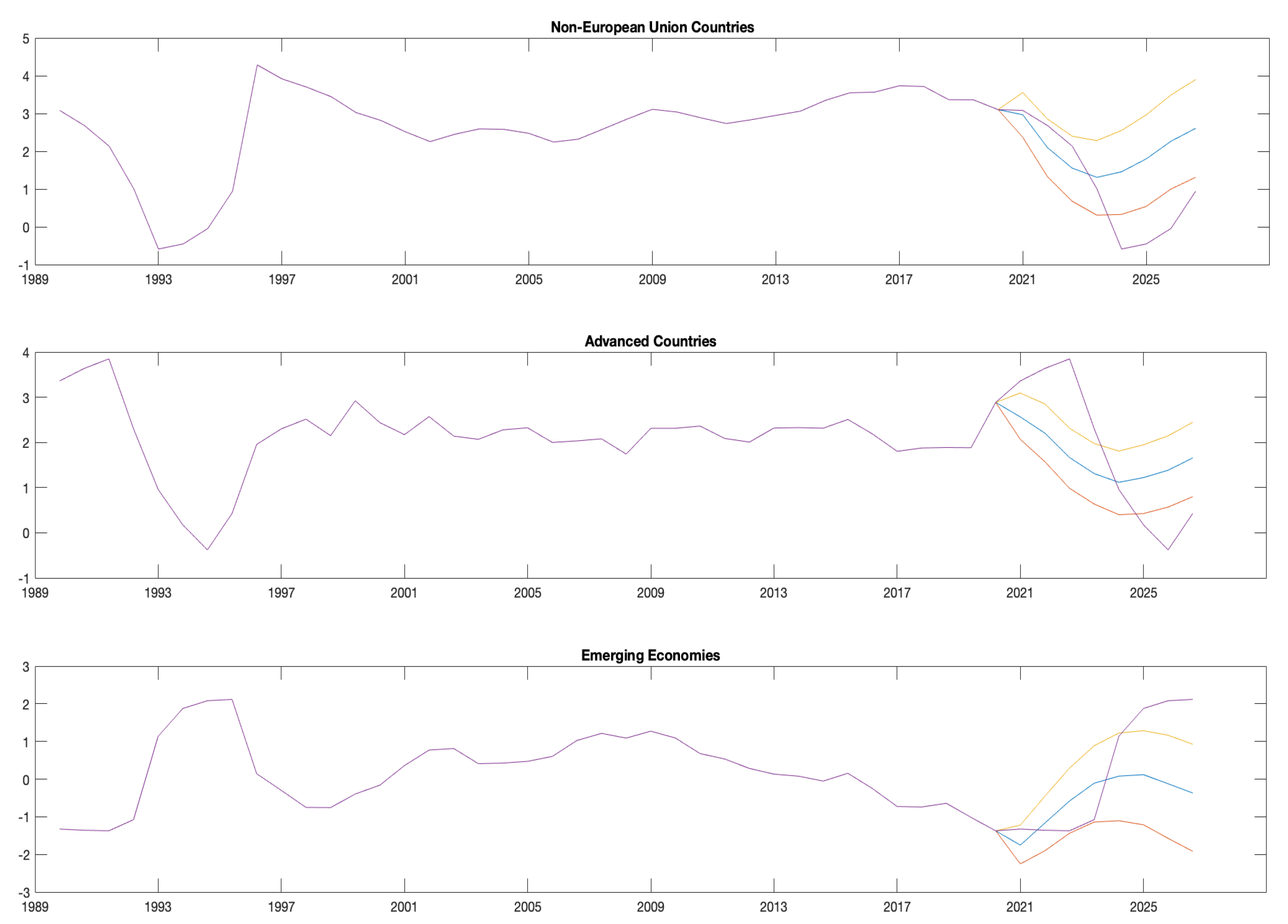
Conditional density forecasts are displayed in Figure 3 to summarise and highlight the main previous findings. A total of 1000 retained replications has been used to conduct posterior inference at each t, where the convergence has been obtained by amounting about to 1 draw per regression parameter. I recall that the outcomes absorb the conditional forecasts computed for a time frame of 2 years (8 quarters), and the natural conjugate prior refers to the three subsamples: (i) $2006q1$–$2009q4$, according to the Great Recession; (ii) $2010q1$–$2018q4$, dealing with postcrisis fiscal consolidation periods; and (iii) $2019q4$–$2021q1$, investigating further volatility changes due to the ongoing pandemic disease. In Figure 3, the yellow and red curves denote the $95\%$ confidence bands, and the blue and purple curves denote the conditional and unconditional projections of outcomes $Y_T$ for each N country indexes and T time periods.

From a modelling perspective, three main findings are addressed. (i) Advanced and non-European Union countries show similar spillovers’ dynamics (top- and middle-plot), but with different spreading and intensity (endogeneity issues). (ii) Conversely to unconditional projections, the conditional ones lie in the confidence interval highlighting better forecasting accuracy. Thus, when investigating international spillovers and dynamic feedback in a challenging unified framework, different set of variables need to be dealt with (misspecified dynamics due to cross-country linkages). (iii) Mostly outward countries’ responses in AVE and NEU emphasize their role in driving the transmission of (global) unexpected shocks, and then their stringent economic recovery, even if uneven and—sometimes—overstrict (misspecified dynamics due to structural breaks).

From a policy perspective, the results highlight greater caution to fine-tune the economy via policy measures and boost productivity to potential growth via accurate structural reforms. In this context, a hint of boosting productivity to potential (even if lower) growth can be observed among countries in the next years, mainly among advanced and non-European Union countries. It highlights strong heterogeneity in economy to be managed carefully, affecting inter-related production and consumption activities that would aid in determining how cross-country recovery resources need to be allocated.

5. Simulated Experiment and Forecasting Accuracy

In this section, a simulated experiment is addressed to highlight and discuss the performance of the estimating procedure of $CSU{R}_v$ model in (8) by using Monte Carlo simulations. Four additional related models are accounted for: (i) Structural Panel Bayesian VAR with Multivariate Time-varying Volatility (SPBVAR-MTV) as in Pacifico (2021), where volatility changes are not replaced by coefficient changes but integrated out; (ii) $CSU{R}_{nv}$ model, with constant volatility; (iii) BCVAR as in Koop et al. (2019), with stocastic volatility; and (iv) Factor-Augmented VAR (FAVAR) as in Bernanke et al. (2005), with volatility changes.

Here, some considerations are in order. In the former (SPBVAR-MTV), (potential) structural breaks, even if treated—by construction—as permament shifts, are re-evaluated at each time period. Thus, in contrast to $CSU{R}_v$, excess spillover effects on outcomes would be more stressed. As regards $CSU{R}_{nv}$, the variance-covariance matrix of ${ϵ}_{i,t}$ is homoscedastic ($\Omega$) and then volatility changes are missing. According to BCVAR, non-informative priors are used to obtain analytical posteriors for both $\Omega$ and ${\sigma }_i^2$. In that context, $\Omega$ would be modelled through a triangular decomposition and ${\sigma }_i^2$ would stand for volatility changes observed in the vector ${\omega }_{i,t}\sim N(0,I_N)$. Finally, FAVAR model is obtained by selecting the optimal (best) number of factors through principal component methods and using non-informative priors to perform forecasting.

According to model features in Section 2.3, a relatively large value for the lag length ($l=5$) is chosen for all methods with no intercept. Then, two distinct sets are constructed: a training set by simulating 120 variables as independent standard normal vectors for $N=15$ and $T=100$ time-series data; and a prediction set by generating 100 additional observations in the same manner. Let the thrust of this analysis be to measure forecasting accuracy and estimating process performance of the proposed methodology, I estimate every model by keeping its framework. More precisely, stacking for all supposed variables,

*

SBCPVAR model for $CSU{R}_v$ and $CSU{R}_{nv}$:

$$Y_{i,t}^{\underset{¯}{S}}=A_{i,j}^{\underset{¯}{S}}\left(L\right)Y_{i,t-\lambda }^{\underset{¯}{S}}+B_{i,j}^{\underset{¯}{S}}\left(L\right)Z_{i,t-\lambda }^{\underset{¯}{S}}+{\epsilon }_{i,t}^{\underset{¯}{S}},$$

where ${}_{\underset{¯}{S}}$ stands for ‘simulated’ and the 120 supposed variables are split for $Y_{i,t-\lambda }^{\underset{¯}{S}}$ and $Z_{i,t-\lambda }^{\underset{¯}{S}}$ equally (60 supposed predictors for each composed vector). Thus, the (simulated) estimation sample amounts, without restrictions, to 900,000 regression parameters, with $K=Nk=15$·$[60+60]·5$.

*

SPBVAR-MTV model:

$$Y_{i,t}^{\underset{¯}{S}}=A_{i,j}^{\underset{¯}{S}}\left(L\right)Y_{i,t-\lambda }^{\underset{¯}{S}}+B_{i,j}^{\underset{¯}{S}}\left(L\right)W_{i,t-\lambda }^{\underset{¯}{S}}+{\ddot{B}}_{i,j}^{\underset{¯}{S}}\left(L\right){\ddot{W}}_{i,t-\lambda }^{\underset{¯}{S}}+C_{i,j}^{\underset{¯}{S}}\left(L\right)Z_{i,t-\lambda }^{\underset{¯}{S}}+{\epsilon }_{i,t}^{\underset{¯}{S}},$$

where the 120 supposed variables are split for $Y_{i,t-\lambda }^{\underset{¯}{S}}$, $W_{i,t-\lambda }^{\underset{¯}{S}}$, ${\ddot{W}}_{i,t-\lambda }^{\underset{¯}{S}}$, and $Z_{i,t-\lambda }^{\underset{¯}{S}}$ equally (30 supposed predictors for each vector). In this context, ${\epsilon }_{i,t}\sim i.i.d.N(0,{\Sigma }_t^{\underset{¯}{S}})$, with ${\Sigma }_t^{\underset{¯}{S}}=diag\left(exp(h_{1t}^{\underset{¯}{S}}),exp(h_{2t}^{\underset{¯}{S}}),\dots ,exp(h_{Nt}^{\underset{¯}{S}})\right)$ and $h_t^{\underset{¯}{S}}={(h_{1t}^{\underset{¯}{S}},h_{2t}^{\underset{¯}{S}},\dots ,h_{Nt}^{\underset{¯}{S}})}^{{}^{\prime }}$ denoting the (simulated) time-varying log-volatilities stacked for i, with $K=Nk=15·[30+30+30+30]·5$.

*

BCVAR model:

$$Y_{i,t}^{\underset{¯}{S}}={\ddot{\Theta }}_{i,t}^{\underset{¯}{S}}\left({\ddot{\Phi }}_i{\ddot{Z}}_{i,t}^{\underset{¯}{S}}\right)+{\sigma }_{i,t}^{\underset{¯}{S}}{\omega }_{i,t},$$

where ${\ddot{\Theta }}_{i,t}^{\underset{¯}{S}}$ contains matrices of coefficients concerning (simulated) lagged outcomes and elements of ${\Omega }^{\underset{¯}{S}}$ obtained by following a triangular decomposition, ${\ddot{\Phi }}_i$ refers to the randomly projection matrix shrinking the parameter space, ${\ddot{Z}}_{i,t}^{\underset{¯}{S}}$ is a vector containing the observable (simulated) outcomes observed at time t and $t-\lambda$, and ${\sigma }_{i,t}^{\underset{¯}{S}}$ denotes the (simulated) standard deviations of the volatilities associated to the vector ${\omega }_{i,t}\sim N(0,I_N)$8, with $N=K$.

*

FAVAR model:

$${\tilde{Y}}_{i,t}^{\underset{¯}{S}}={\Lambda }_{i,j}^{\underset{¯}{S}}{\ddot{F}}_{i,t-\lambda }^{\underset{¯}{S}}+{\ddot{\epsilon }}_{i,t}^{\underset{¯}{S}},$$

where ${\tilde{Y}}_{i,t}^{\underset{¯}{S}}$ follows a VAR(l) process, ${\Lambda }_{i,j}^{\underset{¯}{S}}$ denotes the matrix of coefficients concerning (simulated) lagged outcomes, ${\ddot{F}}_{i,t-\lambda }^{\underset{¯}{S}}$ refers to the vector of lagged (simulated) outcomes, and ${\ddot{\epsilon }}_{i,t}^{\underset{¯}{S}}\sim N\left(0,{\Sigma }^{{\tilde{Y}}_{i,t}^{\underset{¯}{S}}}\right)$, with $N=K$.

Forecasting accuracy is performed by computing the multivariate Weighted Mean Squared Forecast Error ($WMSF{E}_{ij,\tilde{h}}$), with $\tilde{h}\in \{1,2,3,4,8\}$ referring to the step-ahead predictive density forecasts evaluated at ($t-1,T$). It is so obtained:

$$WMSF{E}_{ij,\tilde{h}}=\frac{{\sum }_{t=t-1}^{T+\tilde{h}}w{e}_{ij,T+\tilde{h}}}{{\sum }_{t=t-1}^{T+\tilde{h}}w{e}_{bmk,T+\tilde{h}}},$$

where $w{e}_{ij,T+\tilde{h}}=(e_{ij,T+\tilde{h}}^{{}^{\prime }}·w_{\left|\varphi \right|}·e_{ij,T+\tilde{h}})$ and $w{e}_{bmk,T+\tilde{h}}=(e_{bmk,T+\tilde{h}}^{{}^{\prime }}·w_{\left|\varphi \right|}·e_{bmk,T+\tilde{h}})$ denote the weighted forecast errors of every simulated model and the benchmark one at time $T+\tilde{h}$, respectively, $e_{ij,T+\tilde{h}}$ and $e_{bmk,T+\tilde{h}}$ are the ($K·1$) vector of forecast errors, and $w_{\left|\varphi \right|}$ refers to the PIPs in order to put more weight on large errors. The benchmark model used in this analysis corresponds to a VAR(1) process with constant volatility and no cross-unit lagged interdependencies and structural time variations. It has the form:

$$Y_t=a_0+A_1{Y}_{t-1}+{\epsilon }_t,$$

(21)

where $Y_t={(y_{1t},y_{2t},\dots ,y_{nt})}^{{}^{\prime }}$ is a $n·1$ vector of time-varying outcomes for each i at time t, with $i=1,2,\dots ,n$ denoting the country index, $a_0$ denotes intercepts, $A_1$ is a $n\times n$ matrix of lagged coefficients for each i, $Y_{t-1}$ is a $n·1$ vector of lagged outcomes for each i at time $t-1$ (only one lag), and ${\epsilon }_t\sim N(0,\Omega )$ is a $n·1$ unobserved white noise vector process serially uncorrelated (or independent) with zero mean and time invariant covariance matrix ($\Omega$). Because of each equation has the same regressors (lagged values of $y_{it}$), the VAR(1) in (21) can be just written as a SUR model with lagged variables and deterministic terms as common regressors so as to be compared with every supposed model.

Table 2. Forecasting Accuracy.

Forecast	FAVAR	SPBVAR-MTV	BCVAR	${\mathit{CSUR}}_{\mathit{nv}}$	${\mathit{CSUR}}_{\mathit{v}}$
$\tilde{h}=1$	1.053	1.046	0.931 **	0.932 **	0.904 ***
$\tilde{h}=2$	1.037	1.021	0.939 *	0.929 **	0.898 ***
$\tilde{h}=3$	1.028	1.019	0.957	0.965	0.913 **
$\tilde{h}=4$	1.025	1.013	0.974	0.981	0.927 **
$\tilde{h}=8$	1.010	1.004	0.981	0.998	0.908 ***

The first column denotes the $\tilde{h}$-step-ahead predictive density forecasts evaluated at (t − 1, T), and the remaining five columns refer to the (theoretical) $WMSF{E}_{ij,\tilde{h}}$ estimates computed for every supposed model. The significance codes stand for: (*) significance at 10%; (**) significance at 5%; and (***) significance at 1%.

displays the (theoretical) $WMSF{E}_{ij,\tilde{h}}$ estimates computed simulating all five supposed models with respect to the benchmark one displayed in (21). Four main findings are addressed. (i) According to absence of volatility changes (such as $CSU{R}_{nv}$), lower weighted forecast errors are obtained than high dimensional multicountry data (such as FAVAR and SPBVAR-MTV), by reaching a not bad significance for the first two periods ahead. Thus, a compressed regression in shrinkage of large parameter and model spaces tend to perform better. (ii) Bayesian random compression method with stochastic volatility (such as BCVAR) shows significant estimates in the short-term and results close to the $CSU{R}_{nv}$ ones, highlighting the need to impose a robust Bayesian model averaging procedure when modelling time-varying and inter-related factors. (iii) Multivariate time-varying volatilities (such as SPBVAR-MTV) performs better than FAVAR but worse than Bayesian compressed methods due to its quite expensive associated computational costs compared to huge estimation sample (≥35,000)9. (iv) The lowest weighted forecast errors are displayed in the $CSU{R}_v$ model according to its hierarchical (structural) prior specification strategy and shrinking process. Thus, the most amount of variability (or dispersion) is adequately explained from the estimating procedure. In addition, let the framework be multidimensional (panel data analysis), it would perform better dealing for either endogeneity or valitility issues.

6. Concluding Remarks

This paper improves the Bayesian compressed regression literature concerning VAR models with time-varying parameters and stochastic volatilities. The proposed methodology is obtained by combining and implementing the underlying logic in the Pacifico (2020b)’s analysis, which highlights the need to select the best subset of predictors through MCMC-based Posterior Model Probabilities rather than random draws, and the estimating procedure used in Pacifico (2021), by jointly modelling high dimensional parameter and model spaces. Multivariate Conjugate Informative Proper Mixture priors are addressed to select the best model solution (or combination of predictors) fitting the data, acting as a strong model selection in large model classes. Finally, MCMC algorithms are used to construct exact posterior distributions and shrink jointly VAR parameters and volatility elements in order to perform accurate cross-country forecasts and policy issues.

An empirical application is developed by accounting for a large set of macroeconomic–financial and socioeconomic–demographic variables to highlight the performance of the methodology proposed in this study. Thus, conditional density forecasts and strategic policy measures investigating either the impact of COVID-19 pandemic or real/financial shocks on the economic activity are performed.

A simulated experiment—compared to related works—is also addressed to discuss theoretical properties and forecasting accuracy through Monte Carlo simulations. The findings prove that the hierarchical (structural) prior specification strategy and shrinking process perform lower weighted forecast errors and then better conditional density forecasts when studying large set of time-varying data with policy shifts and volatility changes.

References

- Andrews, Donald W. K. 1991a. Asymptotic normality of series estimators for nonparametric and semiparametric regression models. Econometrica 59: 307–45. [Google Scholar] [CrossRef]
- Andrews, Donald W. K. 1991b. Heteroskedasticity and autocorrelation consistent covariance matrix estimation. Econometrica 59: 817–58. [Google Scholar] [CrossRef]
- Banbura, Marta, Domenico Giannone, and Lucrezia Reichlin. 2010. Large bayesian vector autoregressions. Journal of Applied Econometrics 25: 71–92. [Google Scholar] [CrossRef]
- Bernanke, Ben S., Jean Boivin, and Piotr Eliasz. 2005. Measuring monetary policy: A factor augmented vector autoregressive (favar) approach. The Quarterly Journal of Economics 120: 387–422. [Google Scholar]
- Canova, Fabio, and Fernando J. Pérez Forero. 2015. Estimating overidentified, nonrecursive, time-varying coefficients structural vector autoregressions. Quantitative Economics 6: 359–84. [Google Scholar] [CrossRef] [Green Version]
- Canova, Fabio, and Matteo Ciccarelli. 2009. Estimating multicountry var models. International Economic Review 50: 929–59. [Google Scholar] [CrossRef] [Green Version]
- Canova, Fabio, and Matteo Ciccarelli. 2016. Panel vector autoregressive models: A survey. Advances in Econometrics 32: 205–46. [Google Scholar]
- Carriero, Andrea, George Kapetanios, and Massimiliano Marcellino. 2009. Forecasting exchange rates with a large bayesian var. International Journal of Forecasting 25: 400–17. [Google Scholar] [CrossRef] [Green Version]
- Carriero, Andrea, Todd E. Clark, and Massimiliano Marcellino. 2015a. Bayesian vars: Specification choices and forecast accuracy. Journal of Applied Econometrics 30: 46–73. [Google Scholar] [CrossRef]
- Carriero, Andrea, Todd E. Clark, and Massimiliano Marcellino. 2015b. Large Vector Autoregressions with Asymmetric Priors and Time Varying Volatilities. Working Paper. Brisbane: School of Economics and Finance, vol. 759, pp. 1–34. Available online: http://hdl.handle.net/10419/130773 (accessed on 1 July 2022).
- Carriero, Andrea, Todd E. Clark, and Massimiliano Marcellino. 2016. Common drifting volatility in large bayesian vars. Journal of Business and Economic Statistics 34: 375–90. [Google Scholar] [CrossRef]
- Carriero, Andrea, Todd E. Clark, and Massimiliano Marcellino. 2019. Large bayesian vector autoregressions with stochastic volatility and non-conjugate priors. Journal of Econometrics 212: 137–54. [Google Scholar] [CrossRef]
- Christoffersen, Peter F., and Francis X. Diebold. 1998. Cointegration and long-horizon forecasting. Journal of Business and Economic Statistics 16: 450–58. [Google Scholar]
- Ciccarelli, Matteo, Eva Ortega, and Maria T. Valderrama. 2018. Commonalities and cross-country spillovers in macroeconomic-financial linkages. Journal of Macroeconomics 16: 231–75. [Google Scholar] [CrossRef]
- Clark, Todd E. 2011. Real-time density forecasts from bayesian vector autoregressions with stochastic volatility. Journal of Business and Economic Statistics 29: 327–41. [Google Scholar] [CrossRef]
- Clark, Todd E., and Francesco Ravazzolo. 2015. Macroeconomic forecasting performance under alternative specifications of time-varying volatility. Journal of Applied Econometrics 30: 551–75. [Google Scholar] [CrossRef]
- Cogley, Timothy, and Thomas J. Sargent. 2005. Drifts and volatilities: Monetary policy and outcomes in the post wwii u.s. Review of Economic Dynamics 8: 262–302. [Google Scholar] [CrossRef] [Green Version]
- Cogley, Timothy, Sergei Morozov, and Thomas J. Sargent. 2005. Bayesian fan charts for uk inflation: Forecasting and sources of uncertainty in an evolving monetary system. Journal of Economic Dynamics and Control 29: 1893–925. [Google Scholar] [CrossRef] [Green Version]
- Cuaresma, Jesús Crespo, Martin Feldkircher, and Florian Huber. 2016. Forecasting with global vector autoregressive models: A bayesian approach. Journal of Applied Econometrics 31: 1371–91. [Google Scholar] [CrossRef]
- Curcio, Domenico, Rosa Cocozza, and Antonio Pacifico. 2020. Do global markets imply common fear? Rivista Bancaria—Minerva Bancaria 2020: 1–24. [Google Scholar]
- D’Agostino, Antonello, Luca Gambetti, and Domenico Giannone. 2013. Macroeconomic forecasting and structural change. Journal of Applied Econometrics 28: 82–101. [Google Scholar] [CrossRef] [Green Version]
- Dées, Stéphane, Filippo Di Mauro, M. Hashem Pesaran, and L. Vanessa Smith. 2007. Exploring the international linkages of the euro area: A global var analysis. Journal of Applied Econometrics 22: 1–38. [Google Scholar] [CrossRef] [Green Version]
- Dovern, Jonas, Martin Feldkircher, and Florian Huber. 2016. Does joint modelling of the world economy pay off? evaluating global forecasts from a bayesian gvar. Journal of Economic Dynamics and Control 70: 86–100. [Google Scholar] [CrossRef] [Green Version]
- Feldkircher, Martin, and Florian Huber. 2016. The international transmission of us shocks—Evidence from bayesian global vector autoregressions. European Economic Review 81: 167–88. [Google Scholar] [CrossRef]
- Gelfand, Alan E., and Dipak K. Dey. 1994. Bayesian model choice: Asymptotics and exact calculations. Journal of the Royal Statistical Society: Series B 56: 501–14. [Google Scholar]
- George, Edward I., Dongchu Sun, and Shawn Ni. 2008. Bayesian stochastic search for var model restrictions. Journal of Econometrics 142: 553–80. [Google Scholar] [CrossRef] [Green Version]
- Giannone, Domenico, Michele Lenza, and Giorgio E. Primiceri. 2015. Prior selection for vector autoregressions. The Review of Economics and Statistics 97: 436–51. [Google Scholar] [CrossRef] [Green Version]
- Götz, Thomas, and Erik Haustein. 2018. Bayesian compression for mixed frequency vector autoregressions: A forecast study for germany. SSRN, 1–36. [Google Scholar] [CrossRef]
- Guhaniyogi, Rajarshi, and David B. Dunson. 2015. Bayesian compressed regression. Journal of the American Statistical Association 110: 1500–14. [Google Scholar] [CrossRef]
- Hansen, Bruce E. 1992. Tests for parameter instability in regressions with i(1) processes. Journal of Business and Economic Statistics 10: 321–35. [Google Scholar]
- Huber, Florian. 2016. Density forecasting using bayesian global vector autoregressions with stochastic volatility. International Journal of Forecasting 32: 818–37. [Google Scholar] [CrossRef]
- Jacquier, Eric, Nicholas G. Polson, and Peter E. Rossi. 1994. Bayesian analysis of stochastic volatility. Journal of Business and Economic Statistics 12: 371–417. [Google Scholar]
- Kadiyala, Rao K., and Sune Karlsson. 1997. Numerical methods for estimation and inference in bayesian var models. Journal of Applied Econometrics 12: 99–132. [Google Scholar] [CrossRef]
- Koop, Gary. 2013. Forecasting with medium and large bayesian vars. Journal of Applied Econometrics 28: 177–203. [Google Scholar] [CrossRef] [Green Version]
- Koop, Gary, and Dimitris Korobilis. 2009. Bayesian multivariate time series methods for empirical macroeconomics. Foundations and Trends in Econometrics 3: 267–358. [Google Scholar] [CrossRef]
- Koop, Gary, and Dimitris Korobilis. 2013. Large time-varying parameter vars. Journal of Econometrics 177: 185–98. [Google Scholar] [CrossRef] [Green Version]
- Koop, Gary, and Dimitris Korobilis. 2016. Model uncertainty in panel vector autoregressive models. European Economic Review 81: 115–31. [Google Scholar] [CrossRef] [Green Version]
- Koop, Gary, Dimitris Korobilis, and Davide Pettenuzzo. 2019. Bayesian compressed vector autoregressions. Journal of Econometrics 210: 135–54. [Google Scholar] [CrossRef] [Green Version]
- Korobilis, Dimitris. 2016. Prior selection for panel vector autoregressions. Computational Statistics and Data Analysis 101: 110–20. [Google Scholar] [CrossRef] [Green Version]
- Madigan, David, and Adrian E. Raftery. 1994. Model selection and accounting for model uncertainty in graphical models using occam’s window. Journal of American Statistical Association 89: 1535–46. [Google Scholar] [CrossRef]
- Madigan, David, Jeremy York, and Denis Allard. 1995. Bayesian graphical models for discrete data. International Statistical Review 63: 215–32. [Google Scholar] [CrossRef] [Green Version]
- Mullainathan, Sendhil, and Jann Spiess. 2017. Machine learning: An applied econometric approach. Journal of Economic Perspectives 31: 87–106. [Google Scholar] [CrossRef] [Green Version]
- Pacifico, Antonio. 2019. Structural panel bayesian var model to deal with model misspecification and unobserved heterogeneity problems. Econometrics 7: 8. [Google Scholar] [CrossRef] [Green Version]
- Pacifico, Antonio. 2020a. Fiscal implications, misspecified dynamics, and international spillover effects across europe: A time-varying multicountry analysis. International Journal of Statistics and Economics 21: 18–40. [Google Scholar]
- Pacifico, Antonio. 2020b. Robust open bayesian analysis: Overfitting, model uncertainty, and endogeneity issues in multiple regression models. Econometric Reviews 40: 148–76. [Google Scholar] [CrossRef]
- Pacifico, Antonio. 2021. Structural panel bayesian var with multivariate time-varying volatility to jointly deal with structural changes, policy regime shifts, and endogeneity issues. Econometrics 9: 20. [Google Scholar] [CrossRef]
- Pesaran, M. Hashem, Til Schuermann, and Vanessa L. Smith. 2009. Forecasting economic and financial variables with global vars. International Journal of Forecasting 25: 642–75. [Google Scholar] [CrossRef] [Green Version]
- Pesaran, M. Hashem, Til Schuermann, and Scott M. Weiner. 2004. Modeling regional interdependencies using a global error-correcting macroeconometric model. Journal of Business and Economic Statistics 22: 129–62. [Google Scholar] [CrossRef]
- Primiceri, Giorgio E. 2005. Time varying structural vector autoregressions and monetary policy. Review of Economic Studies 72: 821–52. [Google Scholar] [CrossRef]
- Quintos, Carmela E., and Peter C. B. Phillips. 1993. Parameter constancy in cointegrating regressions. Empirical Economics 18: 675–706. [Google Scholar] [CrossRef]
- Raftery, Adrian E., David Madigan, and Chris T. Volinsky. 1995. Accounting for model uncertainty in survival analysis improves predictive performance. Bayesian Statistics 6: 323–49. [Google Scholar]
- Raftery, Adrian E., David Madigan, and Jennifer A. Hoeting. 1997. Bayesian model averaging for linear regression models. Journal of American Statistical Association 92: 179–91. [Google Scholar] [CrossRef]
- Sofer, Tamar, Lee Dicker, and Xihong Lin. 2014. Variable selection for high dimensional multivariate outcomes. Statistica Sinica 24: 1633–54. [Google Scholar] [CrossRef] [PubMed] [Green Version]
- Taveeapiradeecharoen, Paponpat, and Nattapol Aunsri. 2020. A time-varying bayesian compressed vector autoregression for macroeconomic forecasting. IEEE Access 8: 192777–86. [Google Scholar]
- Taveeapiradeecharoen, Paponpat, Chamnongthai Kosin, and Nattapol Aunsri. 2019. Bayesian compressed vector autoregression for financial time-series analysis and forecasting. IEEE Access 7: 16777–86. [Google Scholar] [CrossRef]
Figure 1.
Systemic Contributions of the given a shock to the variables within the system are drawn as standard deviations and split in the three cross-country variable groups: economic status (ECOST); socioeconomic–demographic factors (SOCDEM); and macroeconomic–financial variables (ECOFIN). All estimates are expressed in posterior means and refer to country–specific (plot a), common (plot b), and variable–specific (plot c) spillover effects.
Figure 2.
Systemic Contributions of the given a shock to the variables within the system are drawn as standard deviations and split in the three cross-country variable groups: economic status (ECOST); socioeconomic–demographic factors (SOCDEM); and macroeconomic–financial variables (ECOFIN). All estimates are expressed in posterior means and refer to crisis and postcrisis periods dealing with common spillover effects through (plot a) and (plot b) models.
Figure 3.
The plot draws density forecasts for outcomes () split in the three country groups: non-European Union countries; advanced countries; and emerging economies. All time-varying parameters are posterior means and correspond to conditional (blue line) and unconditional (purple line) projections of every best predictor evaluated through the model in (8).