Two-Step Lasso Estimation of the Spatial Weights Matrix

Abstract

The vast majority of spatial econometric research relies on the assumption that the spatial network structure is known a priori. This study considers a two-step estimation strategy for estimating the $n(n-1)$ interaction effects in a spatial autoregressive panel model where the spatial dimension is potentially large. The identifying assumption is approximate sparsity of the spatial weights matrix. The proposed estimation methodology exploits the Lasso estimator and mimics two-stage least squares (2SLS) to account for endogeneity of the spatial lag. The developed two-step estimator is of more general interest. It may be used in applications where the number of endogenous regressors and the number of instrumental variables is larger than the number of observations. We derive convergence rates for the two-step Lasso estimator. Our Monte Carlo simulation results show that the two-step estimator is consistent and successfully recovers the spatial network structure for reasonable sample size, T.

1. Introduction

This study proposes an estimator, based on the Lasso estimator, for an approximately sparse spatial weights matrix in a high-dimensional setting. The vast majority of spatial econometric research relies on the assumption that the spatial weights matrix, ${\mathrm{W}}_n$, which measures the strength of interactions between units, is known a priori. In applied work, researchers often need to select between standard specifications such as the binary contiguity matrix, inverse distance matrix or other matrices based on some observable notion of distance. The choice of spatial weights has been a focus of criticism of spatial econometric methods, since estimation results highly depend on the researcher’s specification of the spatial weights matrix [1,2,3]. Furthermore, a pre-defined weights matrix does not provide insights into the drivers of socio-economic interactions and general equilibrium effects in a network, but only allows for measuring the general strength of interactions, which is reflected in the size of the spatial autoregressive coefficient.

The shortcomings of employing pre-specified spatial weights are well known. Pinkse et al. [4] is one of the first attempts to conduct inferences in a setting where the spatial weights matrix is not known a priori. The authors propose a semi-parametric estimator which relies on observable distance measures. Bhattacharjee and Jensen-Butler [5] consider estimation of the spatial weights matrix from the spatial autocovariance matrix in spatial panel models, and show that ${\mathrm{W}}_n$ is only partially identified. Intuitively, the main issue is that, in contrast to autocovariances, spatial weights relate to the direction and strength of causation between spatial units. Since there are twice as many spatial weights as there are autocovariances, further assumptions are required for identification. Bhattacharjee and Jensen-Butler [5] propose an estimator that provides exact identification under the assumption that the spatial weights matrix is symmetric and n is fixed.1 Estimation of the spatial weights matrix in a low-dimensional small n panel, under different structural assumptions on the autocovariances or using moment conditions is discussed in [7,8].

The aforementioned literature focuses on a low-dimensional context where typically $n\ll T$. In contrast, Bailey et al. [9] consider sparsity of the spatial weights matrix as an alternative identification assumption based on a large T panel setting and the spatial error model. They apply a multiple testing procedure to the matrix of spatial autocorrelation coefficients in order to identify the non-zero interactions, and place weights of $+1$, $-1$ or zero, depending on whether the autocorrelations are significantly positive, significantly negative or insignificant, respectively. There are also a few previous studies which apply Lasso-type estimators to high-dimensional spatial panel models and assume sparsity.2 Manresa [13] considers a non-autoregressive panel model with spatially lagged exogenous regressors. Hence, the model does not suffer from simultaneity and the Lasso estimator can be used for dimensionality reduction. Souza [14] and Lam and Souza [15] consider a spatial autoregressive model with additional spatial lags on exogenous regressors. Souza [14] discusses several exclusion restrictions that allow for identification, but require prior knowledge about the network structure. Lam and Souza [15] propose a Lasso-type estimator for spatial weights under the assumption that the error variance decays to zero as T increases, which may be a strong assumption in some applications. By contrast, the method proposed here does not require prior knowledge about the network structure and does not rely on variance decay, but instead exploits exogenous regressors as instruments.

This study explores the estimation of the spatial weights matrix in a panel data setting where T, the number of time periods, is large. The spatial autoregressive or spatial lag model is given by

$$y_{it}=\sum _{j=1}^n{w}_{ij}{y}_{jt}+{\mathrm{x}}_{it}^{\prime }{\beta }_i+e_{it},t=1,\dots ,T;i=1,\dots ,n$$

(1.1)

where $y_{it}$ is the response variable, ${\mathrm{x}}_{it}={(x_{1,it},x_{2,it},\dots ,x_{K,it})}^{\prime }$ is the vector of exogenous regressors and ${\beta }_i$ is the $K\times 1$ parameter vector with $K\ge 1$. The error term is assumed to be independently distributed, but allowed to be heteroskedastic and non-Gaussian. $w_{ij}$ is the $(i,j)$th element of the $n\times n$ spatial weights matrix, denoted by ${\mathrm{W}}_n$, and measures the strength of spill-over effects from unit j to unit i. The spatial weights matrix has zeros on the diagonal, i.e., $w_{ii}=0$ for all i.3 The first term on the right-hand side is often referred to as the spatial lag, analogous to a temporal lag in time-series models. The spatial autoregressive panel model is a natural extension to cross-sectional spatial autoregressive models as introduced by [16,17]. Spatio-temporal panel models, such as the spatial autoregressive model in (1.1), have recently attracted much attention; see, for example, [18,19,20,21,22].4

Estimation of the above model poses two major challenges when ${\mathrm{W}}_n$ is treated as unknown. First, the model suffers from reverse causality as the response variable appears both on the left and right-hand side of the equation. It is well known that ordinary least squares (OLS) is inconsistent in the presence of endogeneity. Second, the model is not identified unless the number of parameters, $p:=n(n-1)+Kn$, is smaller than the number of observations, $nT$, or further assumptions are made. The identification assumption considered here is sparsity of the weights matrix which requires that each unit is affected by only a limited number of other units. Specifically, the number of units affecting a specific unit i is assumed to be much smaller than T, but we explicitly allow for $p\gg nT$.

The proposed estimation method is a two-step procedure based on the Lasso estimator introduced by Tibshirani [24]. The Lasso is a regularization technique which can, under the sparsity assumption, deal with high-dimensional settings where the number of exogenous regressors is large relative to the number of observations. The ${\ell }_1$-penalization employed by the Lasso sets some of the coefficient estimates to exactly zero, making the Lasso estimator attractive for model selection. The ${\ell }_1$-penalization behaves similarly to the ${\ell }_0$-penalty, as used in the Akaike information criterion and Bayesian information criterion [25,26], but is computationally more attractive due to its convex form. The Lasso is a popular and well-established technique, but its theoretical properties have only recently been better understood. Recent theoretical contributions include [27,28,29,30,31,32,33,34,35].

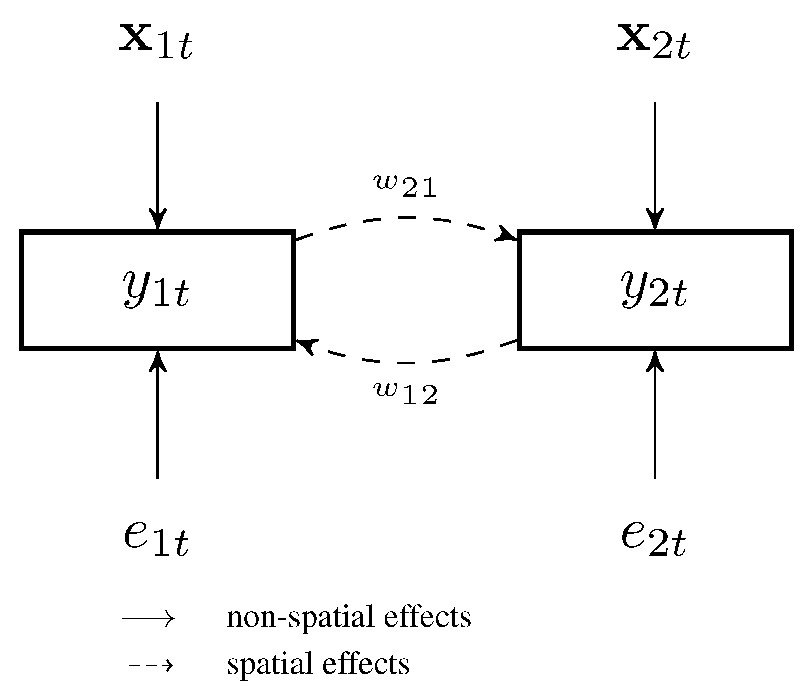
Conceptually, identification of a spatial weights matrix requires suitably dealing with the endogeneity inherent in model (1.1). Lam and Souza [15] address this issue by assuming that the error variance asymptotically decays to zero. By contrast, we address endogeneity using instruments. The estimation methodology proceeds in two steps. In the first step, relevant instruments are identified by the Lasso and predictions for $y_{1t},\dots ,y_{nt}$ are obtained. In the second step, the regression model in (1.1) is estimated, but the spatial lag on the right-hand side is replaced with predictions from the first step. That is, the second-step Lasso selects the neighbours affecting $y_{it}$. The procedure is conceptually based on two-stage least squares (2SLS), but employs the Lasso for selecting relevant instruments in the first step and for selecting relevant spatial lags in the second step. Figure 1 visualizes the spatial autoregressive model in (1.1) for $n=2$ and motivates the choice of instruments exploited to identify the spatial weights. In the regression equation with $y_{1t}$ as the dependent variable, we can exploit ${\mathrm{x}}_{2t}$ as instruments for $y_{2t}$ and vice versa.

Figure 1. The Spatial Autoregressive Model for $n=2$.

Figure 1. The Spatial Autoregressive Model for $n=2$.

We also consider the post-Lasso OLS estimator due to Belloni and Chernozhukov [31], which applies ordinary least squares (OLS) to the model selected by the Lasso and aims at reducing the Lasso shrinkage bias. Although the estimation methodology relies on large T asymptotics, Monte Carlo results suggest that the two-step Lasso estimator is able to recover the spatial network structure if T is as small as 50–100. The estimator may be combined with established large T panel estimators such as the Common Correlated Effects estimator [36,37], which controls for strong cross-sectional dependence, and can be extended to dynamic models including temporal lags of the dependent variable as regressors.

Finally, this study is also related to the emerging literature on high-dimensional methods which allow the number of endogenous regressors to be larger than the sample size. The Self-Tuning Instrumental Variable (STIV) due to Gautier and Tsybakov [38] is a generalization of the Dantzig estimator [39] allowing for many endogenous regressors. The focused generalized methods of moments (FGMM) developed in Fan and Liao [40] extends shrinkage GMM estimators as in, e.g., [41] to high-dimensional settings. The two-step Lasso estimator considered in this study is conceptually similar to Lin et al. [42] who apply two-step penalized least squares to genetic data. We improve upon Lin et al. [42] in that our approach allows for approximate sparsity, non-Gaussian errors and uses the sharper penalty level proposed by Belloni et al. [30]. However, our main contribution is to point out that a simple two-step Lasso estimation method can be employed to estimate the spatial weights matrix. The approach does not require any prior knowledge about the network structure, except for the sparsity assumption and a set of exogenous regressors.

The article is organized as follows. In Section 2, we consider a general setting where the number of endogenous regressors and the number of instruments is allowed to be larger than the number of observations. The two-step estimator may be of more general interest for applications with endogeneity in high-dimensions. Section 3 applies the proposed two-step estimator to estimate the spatial autoregressive model in (1.1). In Section 4, we present Monte Carlo results to demonstrate the performance of the two-step Lasso for estimating the spatial weights matrix. Finally, Section 5 concludes.

Notation. The ${\ell }_q$-norm of the vector $\mathrm{a}\in {\mathbb{R}}^M$ is defined as ${∥\mathrm{a}∥}_q=({\sum }_{m=1}^M|a_m{{|}^q)}^{1/q}$, $q=1,2$. The number of non-zero elements in $\mathrm{a}$ is denoted by ${∥\mathrm{a}∥}_0$, and ${∥\mathrm{a}∥}_{\infty }$ is the largest element in $\mathrm{a}$. We use $((·))$ to denote the typical element of a matrix, e.g., $\mathrm{A}=((a_{ij}))$. The Frobenius norm of $\mathrm{A}$ is ${∥\mathrm{A}∥}_F=({\sum }_{i,j}|a_{ij}{{|}^2)}^{1/2}$. Let ${∥\mathrm{A}∥}_1$ be the entry-wise ${\ell }_1$ norm, i.e., ${∥\mathrm{A}∥}_1={\sum }_{i,j}|a_{ij}|$. The support operator is $\mathrm{supp}(\mathrm{a})=\{m\in \{1,\dots ,M\}:a_m\ne 0\}$. Let V be a set, then $\overline{V}$ is the complement of V. ${\mathrm{a}}_V$ is a vector with elements $a_m\mathbf{1}\{m\in V\}$ for $m=1,\dots ,M$ where $\mathbf{1}$ is the indicator function. The typical element of ${\mathrm{A}}_V$ is $a_{ij}\mathbf{1}\{j\in V\}$. We use $x_T{\lesssim }_{\mathrm{P}}{z}_T$ to denote $x_T=O_P(z_T)$ and $a\lesssim b$ to denote $a\le cb$ for some constant $c>0$.

2. Two-Step Lasso Estimator

In this section, we develop a two-step estimation procedure that allows the number of possibly endogenous regressors as well as the number of instruments to be larger than the sample size. The identifying assumption is approximate sparsity. Section 3 presents the spatial autoregressive model as an application to this setting. The two-step estimator may be of interest in, for example, cross-country growth regressions where the number of regressors is large relative to the number of countries and endogeneity is a potential issue. Furthermore, endogeneity in high dimensions may arise when the aim is to find a sparse linear approximation to a complex non-parametric data-generating process; see earning regressions in [43].

The structural equation and first-step equations are given by

$$\begin{array}{cc}\hfill y_t& ={\mathrm{x}}_t^{\prime }{\beta }^{★}+e_t,\hfill \end{array}$$

(2.1)

$$\begin{array}{cc}\hfill x_{tj}& ={\mathrm{z}}_t^{\prime }{\pi }_j^{★}+u_{tj},j=1,\dots ,p.\hfill \end{array}$$

(2.2)

$y_t$ is the outcome variable and ${\mathrm{x}}_t$ is a p-dimensional vector of regressors. For notational consistency with Section 3, we use $t=1,\dots ,T$ to denote distinct units or repeated observations over time. Without loss of generality, we assume that the first $\overline{p}$ regressors are endogenous, i.e., $\mathrm{E}[e_t|x_{tj}]\ne 0$ for $j=1,\dots ,\overline{p}$ with $\overline{p}\in \{1,\dots ,p\}$. The remaining $p-\overline{p}$ regressors are exogenous. Hence, we allow the set of exogenous regressors to be empty. We assume the existence of $L\ge p$ instruments, ${\mathrm{z}}_t$, which satisfy the exclusion restriction $\mathrm{E}[e_t|{\mathrm{z}}_t]=\mathrm{E}[u_{tj}|{\mathrm{z}}_t]=0$ for $j=1,\dots ,p$. If a regressors $x_{tj}$ is exogenous, it serves as an instrument for itself. Hence, $z_{tj}=x_{tj}$ for $j>\overline{p}$. The error terms $e_t$ and $u_{tj}$ are independently distributed, but possibly heteroskedastic and non-Gaussian. The interest lies in obtaining a sparse approximation of ${\beta }^{★}$. While the model in (2.1)–(2.2) assumes that the conditional expectation functions are linear, the framework may be easily generalized to a non-parametric data-generating process as in, for example, Bickel et al. [27].

2.1. First-Step Estimation

The aim of the first step is to estimate the conditional expectation function $x_{tj}^{★}:=\mathrm{E}[x_{tj}|{\mathrm{z}}_t]={\mathrm{z}}_t^{\prime }{\pi }_j^{★}$ for $j=1,\dots ,\overline{p}$ where $x_{tj}^{★}$ represents the optimal instrument. Note that $x_{tj}^{★}=x_{tj}$ if $x_{tj}$ is exogenous, which corresponds to $j=\overline{p}+1,\dots ,p$. If $L>T$, OLS estimation of the first-step equations in (2.2) is not feasible as the Gram matrix $T^{-1}{\mathrm{Z}}^{\prime }\mathrm{Z}$ with $\mathrm{Z}=((z_{tj}))$ is singular. The Lasso can achieve consistency in a high-dimensional setting where $L>T$ under the assumption of sparsity and further regularity conditions stated below. Exact sparsity requires that the number of nonzero elements in ${\pi }_j^{★}$, i.e., ${\parallel {\pi }_j^{★}\parallel }_0$, is small relative to the sample size. This assumption is too strong in most applications as ${\pi }_j^{★}$ may have many elements that are, although negligible, not exactly zero. Instead, we assume the existence of a sparse parameter vector ${\pi }_j^0$ that approximates the true parameter vector ${\pi }_j^{★}$. Specifically, as in [30], we assume that for each endogenous regressor j the number of instruments necessary for approximating the conditional expectation function is smaller than the sample size and the associated approximation error $a_{tj}({\mathrm{z}}_t)=x_{tj}^{★}-{\mathrm{z}}_t^{\prime }{\pi }_j^0$ converges as specified below.5

Assumption 2.1. 

Consider the model in (2.2). There exists a parameter vector ${\pi }_j^0$ for all $j=1,\dots ,\overline{p}$ such that

$$\mathrm{E}[x_{tj}|{\mathrm{z}}_t]={\mathrm{z}}_t^{\prime }{\pi }_j^0+a_{tj}({\mathrm{z}}_t),s_1:=\underset{1\le j\le \overline{p}}{max}{\parallel {\pi }_j^0\parallel }_0\ll T,A_{s_1}:=\underset{1\le j\le \overline{p}}{max}\sqrt{\frac{1}{T}\sum _{t=1}^T{a}_{tj}^2}{\lesssim }_{\mathrm{P}}\sqrt{\frac{s_1}{T}}$$

The target parameter ${\pi }_j^0$ can be motivated as the solution to the infeasible oracle program that penalizes the number of non-zero parameters [31]. Under homoskedasticity, we can write the oracle objective function as

$$\underset{{\pi }_j}{min}\frac{1}{T}{∥{\mathrm{X}}_j-\mathrm{Z}{\pi }_j∥}_2^2+\frac{{\sigma }^2}{T}{\parallel {\pi }_j\parallel }_0$$

where ${\mathrm{X}}_j$ is the jth column of the matrix $\mathrm{X}=((x_{tj}))$. The second term represents the noise level and $\sqrt{s_1/T}$ is the convergence rate of the oracle which knows the true model.

The first-step Lasso estimator for endogenous regressor j is defined as

$${\widehat{\pi }}_j=argmin\frac{1}{T}{∥{\mathrm{X}}_j-\mathrm{Z}{\pi }_j∥}_2^2+\frac{{\lambda }_1}{T}{∥{\widehat{\mathsf{{\rm Y}}}}_{1j}{\pi }_j∥}_1$$

The first term is the residual sum of squares and the second term imposes a penalty on the absolute size of the parameters which is increasing in the penalty level ${\lambda }_1$. The Lasso nests OLS with ${\lambda }_1=0$ and ${\lambda }_1=\infty$ will lead to a null model. ${\widehat{\mathsf{{\rm Y}}}}_{1j}$ is a diagonal matrix of penalty loadings which account for heteroskedasticity and may be set to the identity matrix under homoskedasticity [30]. The second term imposes a penalty on the absolute size of the coefficients and, thus, shrinks the coefficient estimates towards zero. The Lasso predictions ${\widehat{\mathrm{X}}}_j:=\mathrm{Z}{\widehat{\pi }}_j$ replace ${\mathrm{X}}_j$ in the second step to address endogeneity. For the exogenous regressors, we set ${\widehat{\mathrm{X}}}_j={\mathrm{X}}_j$.

The penalty level ${\lambda }_1$ may be selected by cross-validation in order to minimize the prediction error as originally suggested by Tibshirani [24]. Since the primary purpose of our study is not prediction, but recovery of the spatial network structure, we follow an alternative approach that originates from Bickel et al. [27]. The penalty level is chosen as the smallest value that, with a high probability, overrules the random part of the data-generating process, which is represented by the score vector ${\mathrm{S}}_{1j}=-\frac{2}{T}{\widehat{\mathsf{{\rm Y}}}}_{1j}^{-1}{\mathrm{Z}}^{\prime }{\mathrm{u}}_j$, i.e.,

$$\frac{{\lambda }_1}{T}\ge c\underset{1\le j\le \overline{p}}{max}{∥{\mathrm{S}}_{1j}∥}_{\infty }\mathrm{with}c>1$$

(2.3)

The event in (2.3) plays a crucial role in the derivation of non-asymptotic bounds and convergence rates. Belloni et al. [30] show with the use of moderate deviation theory in [44] that as $T\to \infty$, $P(c{max}_{1\le j\le \overline{p}}{∥{\mathrm{S}}_{1j}∥}_{\infty }>{\lambda }_1/T)=o_{\mathrm{P}}(1)$ where

$${\lambda }_1=2c\sqrt{T}{\mathsf{\Phi }}^{-1}(1-\alpha /(2L\overline{p}))\mathrm{with}log(1/\alpha )\lesssim log(max(L\overline{p},T))$$

(2.4)

under possibly non-Gaussian and heteroskedastic errors. Note that the term $\overline{p}$ in (2.4) accounts for the number of Lasso regressions in the first step and L is the number of instruments. c is a constant greater than, but close to 1. In applied work, Belloni et al. [45] suggest setting $c=1.1$ and $\alpha =min(1/T,0.05)$.

The optimal penalty loadings are given by

$${\mathsf{{\rm Y}}}_{1j}^0=\mathrm{diag}({\gamma }_{1j,1},\dots ,{\gamma }_{1j,l},\dots ,{\gamma }_{1j,L}),{\gamma }_{1j,l}=\sqrt{\frac{1}{T}\sum _t{z}_{tl}^2{u}_{tj}^2}$$

(2.5)

but are infeasible as $u_{tj}$ is unobserved. Under the iterative Algorithm in Appendix A.2, we can construct asymptotically valid penalty loadings, ${\widehat{\mathsf{{\rm Y}}}}_{1j}$, that are in the probability limit as least as large as the optimal penalty loadings [30].

The properties of the Lasso estimator depend crucially on the Gram matrix $T^{-1}{\mathrm{Z}}^{\prime }\mathrm{Z}$. As stated above, OLS is not feasible if $L>T$ as the Gram matrix is singular, which implies that the minimum eigenvalue is zero,

$$\underset{\delta \ne \mathbf{0}}{min}\frac{{∥\mathrm{Z}\delta ∥}_2}{\sqrt{T}{∥\delta ∥}_2}=0$$

Bickel et al. [27] introduce the restricted eigenvalue

$$\underset{{\parallel {\delta }_{{\overline{\mathsf{\Omega }}}_{1j}}\parallel }_1\le C{\parallel {\delta }_{{\mathsf{\Omega }}_{1j}}\parallel }_1,\delta \ne \mathbf{0}}{min}\frac{{∥\mathrm{Z}\delta ∥}_2}{\sqrt{T}{∥{\delta }_{{\mathsf{\Omega }}_{1j}}∥}_2}$$

which is defined as the minimum over the restricted set ${\parallel {\delta }_{{\overline{\mathsf{\Omega }}}_{1j}}\parallel }_1\le C{\parallel {\delta }_{{\mathsf{\Omega }}_{1j}}\parallel }_1$, where ${\mathsf{\Omega }}_{1j}=\mathrm{supp}({\pi }_j^0)$ and C is a positive constant. The condition ${\parallel {\delta }_{{\overline{\mathsf{\Omega }}}_{1j}}\parallel }_1\le C{\parallel {\delta }_{{\mathsf{\Omega }}_{1j}}\parallel }_1$ holds with high probability and, when it does not hold, it is not required to bound the prediction error norm (see Appendix A.1).

Definition 1. 

Let C and $\overline{\kappa }$ be positive constants and Ω denote the active set. We say that the restricted eigenvalue condition holds for $\mathrm{M}$, if as $T\to \infty$

$${\kappa }_C(\mathrm{M}):=\underset{{\parallel {\delta }_{\overline{\mathsf{\Omega }}}\parallel }_1\le C{\parallel {\delta }_{\mathsf{\Omega }}\parallel }_1,\delta \ne \mathbf{0}}{min}\frac{\sqrt{s}}{\sqrt{T}}\frac{{∥\mathrm{M}\delta ∥}_2}{{∥{\delta }_{\mathsf{\Omega }}∥}_1}\ge \overline{\kappa }>0,s:={\parallel \delta \parallel }_0$$

In the above definition of the restricted eigenvalue the ${\ell }_2$-norm in the denominator is replaced with the ${\ell }_1$-norm using the Cauchy-Schwarz inequality, which allows us to relate the ${\ell }_1$-parameter norm to the ${\ell }_2$-prediction norm. The restricted eigenvalue is closely related to the compatibility constant [46]. Bühlmann and Van de Geer [28] provide an extensive overview of related conditions and their relationship. The restricted eigenvalue conditions hold under general conditions; see, e.g., [27,31,47]. One sufficient condition for the restricted eigenvalue is the restricted sparse eigenvalue condition which requires that any appropriate sub-matrix of the Gram matrix has positive and finite eigenvalues [27].

To accommodate heteroskedasticity, we also define the weighted restricted eigenvalue condition [30],

$${\kappa }_C^{\omega }(\mathrm{M}):=\underset{{\parallel {\mathsf{{\rm Y}}}^0{\delta }_{\overline{\mathsf{\Omega }}}\parallel }_1\le C{\parallel {\mathsf{{\rm Y}}}^0{\delta }_{\mathsf{\Omega }}\parallel }_1,\delta \ne \mathbf{0}}{min}\frac{\sqrt{s}}{\sqrt{T}}\frac{{∥\mathrm{M}\delta ∥}_2}{{\parallel {\mathsf{{\rm Y}}}^0{\delta }_{\mathsf{\Omega }}\parallel }_1}$$

where ${\mathsf{{\rm Y}}}^0$ are the optimal penalty loadings as in (2.5). If the restricted eigenvalue condition holds, the weighted restricted eigenvalue is positive as long as the optimal penalty loadings are bounded away from zero and bounded from above, which we maintain in the following.

With respect to the first-step equations in (2.2), we explicitly state the restricted eigenvalue condition as follows:

Assumption 2.2. 

The Restricted Eigenvalue Condition holds for $\mathrm{Z}$.

Under Assumption 2.1 and 2.2, using the penalty level as in (2.4), assuming the penalty loadings ${\widehat{\mathsf{{\rm Y}}}}_{1j}$ are asymptotically valid, then by Theorem 1 in [30], the ${\ell }_2$-prediction error norm of the Lasso estimator has the following rate of convergence

$$\underset{1\le j\le \overline{p}}{max}\frac{1}{\sqrt{T}}{∥\mathrm{Z}{\widehat{\pi }}_j-\mathrm{Z}{\pi }_j^{★}∥}_2{\lesssim }_{\mathrm{P}}\sqrt{\frac{s_{1}log(max(L\overline{p},T))}{T}}$$

(2.6)

We do not reproduce the proof of Theorem 1 in [30]. However, our main results in Theorem 1 below is a generalization in that we account for the prediction error that arises from the first-step Lasso estimation. The proof is provided in Appendix A.1. The convergence rate in (2.6) is slower than the oracle rate of $\sqrt{s_1/T}$ by a factor of $\sqrt{log(max(L\overline{p},T))}$, which can be interpreted as the cost of not knowing the active set of ${\pi }_j^0$.

2.2. Second-Step Estimation

Since the second-step is infeasible by OLS if $p>T$, we require, as in the first step, approximate sparsity and assumptions on the Gram matrix.

Assumption 2.3. 

Consider the model in (2.1). There exists a parameter vector ${\beta }^0$ such that

$$\mathrm{E}[y_t|{\mathrm{z}}_t]={\mathrm{x}}_t^{★}{}^{\prime }{\beta }^0+r_t({\mathrm{z}}_t),s_2:={\parallel {\beta }^0\parallel }_0\ll T,R_{s_2}:=\sqrt{\frac{1}{T}\sum _{t=1}^T{r}_t^2}\lesssim \sqrt{\frac{s_2}{T}},{\parallel {\beta }^0\parallel }_2{\lesssim }_{\mathrm{P}}{s}_2$$

Assumption 2.4. 

The Restricted Eigenvalue Condition holds for $\widehat{\mathrm{X}}$.

Assumption 2.3 is similar to Assumption 2.1, but assumes ${\parallel {\beta }^0\parallel }_2\lesssim s_2$, which allows us to simplify the expression for the convergence rates. Assumption 2.4 could also be written in terms of the optimal instrument matrix ${\mathrm{X}}^{★}$. Specifically, Assumption 2.4 holds if the restricted eigenvalue holds for ${\mathrm{X}}^{★}$ and ${\parallel \widehat{\mathrm{X}}-{\mathrm{X}}^{★}\parallel }_{\infty }$ is small as specified in [28], Corollary 6.8.

For identification of ${\beta }^0$ we also require, as standard in the IV/GMM literature, that the matrix ${\mathsf{\Pi }}^0=({\pi }_1^0,\dots ,{\pi }_p^0)$ is full column rank.

Assumption 2.5. 

$\mathrm{rank}({\mathsf{\Pi }}^0)=p$.

The second-step Lasso estimator uses the predictions $\widehat{\mathrm{X}}$ as regressors and is defined as

$$\widehat{\beta }=arg\underset{\beta }{min}\frac{1}{T}{∥\mathrm{y}-\widehat{\mathrm{X}}\beta ∥}_2^2+\frac{{\lambda }_2}{T}{∥{\widehat{\mathsf{{\rm Y}}}}_2\beta ∥}_1$$

where the penalty level is set to

$${\lambda }_2=2c\sqrt{T}{\mathsf{\Phi }}^{-1}(1-\alpha /(2p))\mathrm{with}log(1/\alpha )\lesssim log(max(L\overline{p},T))$$

(2.7)

and the penalty loadings are estimated using the algorithm in Appendix A.2.

The crucial difference to the first-step Lasso estimation is that ${\mathrm{X}}^{★}$ is unobservable and we instead use $\widehat{\mathrm{X}}$, which is an estimate that in general deviates from the optimal instrument ${\mathrm{X}}^{★}$. For the two-step Lasso estimator, we consider the prediction bound $1/\sqrt{T}{\parallel \widehat{\mathrm{X}}\widehat{\beta }-{\mathrm{X}}^{★}{\beta }^{★}\parallel }_2$ where predictions obtained using the unknown optimal instrument and the unknown true parameter vector ${\beta }^{★}$ serve as a reference point. Note that, using the triangle inequality,

$$\begin{array}{cc}\hfill \frac{1}{\sqrt{T}}{∥\widehat{\mathrm{X}}\widehat{\beta }-{\mathrm{X}}^{★}{\beta }^{★}∥}_2& =\frac{1}{\sqrt{T}}{∥(\widehat{\mathrm{X}}\widehat{\beta }-\widehat{\mathrm{X}}{\beta }^0)+(\widehat{\mathrm{X}}{\beta }^0-{\mathrm{X}}^{★}{\beta }^0)+({\mathrm{X}}^{★}{\beta }^0-{\mathrm{X}}^{★}{\beta }^{★})∥}_2\hfill \\ & \le \frac{1}{\sqrt{T}}{∥\widehat{\mathrm{X}}\widehat{\beta }-\widehat{\mathrm{X}}{\beta }^0∥}_2+\frac{1}{\sqrt{T}}{∥\widehat{\mathrm{V}}{\beta }^0∥}_2+R_{s_2}\hfill \end{array}$$

where we define $\widehat{\mathrm{V}}=\widehat{\mathrm{X}}-{\mathrm{X}}^{★}$ which has the typical element ${\widehat{v}}_{jt}={\mathrm{z}}_t^{\prime }{\widehat{\pi }}_j-{\mathrm{z}}_t^{\prime }{\pi }_j^{★}$. The bound for the third term is stated in Assumption 2.3. The convergence rate for the second term follows from prediction norm rate of the first-step Lasso in (2.6). The bound for the first term is derived in Appendix A.1. Combining the three bounds, we have the following result.

Theorem 1. 

Consider the model in (2.1)–(2.2). Suppose Assumptions 2.1–2.5 hold. Suppose asymptotically valid penalty loadings are used and the penalty levels ${\lambda }_1$ and ${\lambda }_2$ are set as in (2.4) and (2.7). Then,

$$\frac{1}{\sqrt{T}}{∥\widehat{\mathrm{X}}\widehat{\beta }-{\mathrm{X}}^{★}{\beta }^{★}∥}_2{\lesssim }_{\mathrm{P}}{s}_2^2\sqrt{\frac{s_{1}log(max(L\overline{p},T))}{T}}$$

Furthermore, if $s_1$ and $s_2$, do not depend on T, then

$$\begin{array}{cc}\hfill {∥\widehat{\beta }-{\beta }^0∥}_1& {\lesssim }_{\mathrm{P}}\sqrt{\frac{log(max(L\overline{p},T))}{T}}\hfill \end{array}$$

The proof is provided in Appendix A.1. As expected, the convergence rates of the ${\ell }_2$-prediction norm depend on the degree of sparsity in the first-step and second-step equation. The second part of the theorem is relevant for the spatial panel model in the next section where the sparsity level ($s_1$ and $s_2$) and the dimension of the problem (L and p) depend on the number of units (i.e., n), but not on the time dimension (T).

3. The Spatial Autoregressive Model

This section applies the proposed two-step Lasso procedure to the spatial lag model in (1.1). In Section 3.2, we discuss two extensions to the two-step Lasso estimator; namely, the post-Lasso and thresholded post-Lasso.

3.1. Two-Step Lasso

The structural and reduced form equations can be written as

$$\begin{array}{cc}\hfill {\mathrm{y}}_i& =\sum _{j=1}^n{w}_{ij}^{★}{\mathrm{y}}_j+{\mathrm{X}}_i{\beta }_i^{★}+{\mathrm{e}}_i\hfill \end{array}$$

(3.1)

$$\begin{array}{cc}\hfill {\mathrm{y}}_j& =\sum _{s=1}^n{\mathrm{X}}_s{\pi }_{j,s}^{★}+{\mathrm{u}}_j,i,j=1,\dots ,n\hfill \end{array}$$

(3.2)

where ${\mathrm{y}}_i={(y_{i1},y_{i2},\dots ,y_{iT})}^{\prime }$, $w_{jj}^{★}=0$, and ${\mathrm{X}}_i={({\mathrm{x}}_{i1}^{\prime },\dots ,{\mathrm{x}}_{iT}^{\prime })}^{\prime }$ is the $T\times K$ matrix of exogenous regressors. We assume that $e_{it}$ is independently distributed across t, i.e., $E\left[e_{it}{e}_{is}\right]=0$ for $t\ne s$. The ${}^{★}$-superscripts indicate that we interpret the parameters as the true parameter values.

It is evident that the spatial model in (3.1)–(3.2) is an application of the more general model in (2.1)–(2.2). Specifically, the right-hand side regressors ${\mathrm{y}}_1,\dots ,{\mathrm{y}}_n$ correspond to endogenous regressors and ${\mathrm{X}}_i$ corresponds to the exogenous regressors in (2.1). Furthermore, the set of exogenous instruments is given by ${\mathrm{X}}_1,\dots ,{\mathrm{X}}_n$.

The choice of instruments is closely related to Kelejian and Prucha [48]. To identify the spatial autoregressive parameter, they suggest the use of first and higher order spatial lags of exogenous regressors as instruments for the endogenous spatial lag. As discussed in the Introduction, we use ${\mathrm{X}}_j$ as instruments in order to identify $w_{ij}^{★}$, which represents the causal impact of ${\mathrm{y}}_j$ on ${\mathrm{y}}_i$. Therefore, for identification, we require contemporaneous exogeneity across space:

Assumption 3.1. 

$\mathrm{E}[e_{it}|{\mathrm{x}}_{jt}]=0$ for all $i,j=1,\dots ,n$ and $t=1,\dots ,T$.

In many applications, estimation of (3.1)–(3.2) by 2SLS is not feasible as there appear $n-1+K$ and $nK$ regressors on the right-hand side, respectively, which are both potentially larger than T. In order to exploit the Lasso estimator, we require sparseness as in Section 2.

Assumption 3.2. 

(a) Consider the model in (3.1). There exists a parameter vector ${\mathrm{w}}_i^0=(w_{i1}^0,\dots ,w_{in}^0)$ for all $i=1,\dots ,n$ with $w_{ii}^0=0$ such that

$$\begin{array}{cc}\hfill \mathrm{E}[y_{it}|{\mathrm{x}}_{1t},\dots ,{\mathrm{x}}_{nt}]& =\sum _{j=1}^n{w}_{ij}^0{y}_{jt}^{★}+{\mathrm{x}}_{it}^{\prime }{\beta }_i^0+a_{it}\hfill \\ \hfill s_1+K& \ll T,A_{s_1}:=\underset{1\le i\le n}{max}\sqrt{\frac{1}{T}\sum _{t=1}^T{a}_{it}^2}{\lesssim }_{\mathrm{P}}\sqrt{\frac{s_1}{T}}\hfill \end{array}$$

where $y_{jt}^{★}=\mathrm{E}[y_{jt}|{\mathrm{x}}_{1t},\dots ,{\mathrm{x}}_{nt}]$, $s_1:={max}_{1\le i\le n}{\parallel {\mathrm{w}}_i^0\parallel }_0$ and $K={\parallel {\beta }_i^0\parallel }_0$

(b) Consider the model in (3.2). There exists a parameter vector ${\pi }_{i,j}^0$ for all $i=1,\dots ,n$ such that

$$\begin{array}{cc}\hfill \mathrm{E}[y_{it}|{\mathrm{x}}_{1t},\dots ,{\mathrm{x}}_{nt}]& =\sum _{j\ne i}{\mathrm{x}}_{jt}^{\prime }{\pi }_{i,j}^0+{\mathrm{x}}_{it}^{\prime }{\pi }_{i,i}^0+r_{it}\hfill \\ \hfill s_2+K& \ll T,R_{s_2}:=\underset{1\le i\le n}{max}\sqrt{\frac{1}{T}\sum _{t=1}^T{r}_{it}^2}{\lesssim }_{\mathrm{P}}\sqrt{\frac{s_2}{T}}\hfill \end{array}$$

where $s_2:={max}_{1\le i\le n}{\sum }_{j\ne i}{\parallel {\pi }_{i,j}^0\parallel }_0$ and $K={\parallel {\pi }_{i,i}^0\parallel }_0$

To simplify the exposition and without loss of generality, we assume that ${\beta }_i^0$ does not include any zero elements, implying that all regressors in ${\mathrm{x}}_{it}$ are relevant determinants of the dependent variable $y_{it}$. The assumption also guarantees identification as long as $K\ge 1$.

The sparsity assumptions in Assumption 3.2 (a) and Assumption 3.2 (b) are related. To see this, consider the case where $n=2$. Then, the reduced form equations are given by

$$\begin{array}{c}\hfill {\mathrm{y}}_1={\mathrm{X}}_1{\pi }_{1,1}+{\mathrm{X}}_2{\pi }_{1,2}+{\mathrm{u}}_1\\ \hfill {\mathrm{y}}_2={\mathrm{X}}_1{\pi }_{2,1}+{\mathrm{X}}_2{\pi }_{2,2}+{\mathrm{u}}_2\end{array}$$

with ${\pi }_{2,1}=\frac{w_{21}}{1-w_{12}{w}_{21}}{\beta }_1$, ${\pi }_{1,2}=\frac{w_{12}}{1-w_{12}{w}_{21}}{\beta }_2$, ${\pi }_{1,1}=\frac{1}{1-w_{12}{w}_{21}}{\beta }_1$ and ${\pi }_{2,2}=\frac{1}{1-w_{12}{w}_{21}}{\beta }_2$ where we assume $\left|w_{12}\right|<1$ and $\left|w_{21}\right|<1$. It becomes evident that, if ${\pi }_{1,2}=\mathbf{0}$, then $w_{12}=0$ must hold by assumption given that ${\parallel \beta \parallel }_0=K$. That is, sparseness of the ${\pi }_{i,j}$ parameter vectors as specified in Assumption 3.2 (b) implies sparseness of the ${\mathrm{W}}_n$ matrix in Assumption 3.2 (a) if $n=2$.

We maintain the following basic assumptions regarding the spatial weights matrix.

Assumption 3.3. 

(a) The spatial weights matrix, ${\mathrm{W}}_n^0=((w_{ij}^0;i,j=1,\dots ,n))$, is $n\times n$ with zeros on the diagonal, $w_{ii}=0$. (b) The spatial weights matrix is time-invariant. (c) The row sums are bounded in absolute value, i.e., ${max}_i{\sum }_j|w_{ij}|<1$.

Assumption 3.3 (a) is standard. Assumption 3.3 (b) is required as the identification strategy exploits variation over time to identify the weights matrix and is standard in the spatial panel econometrics literature; see, e.g., [20]. The assumption corresponds to parameter stability over time in time series.6 Assumption 3.3 (c) can be interpreted similar to the stationarity condition in time-series econometrics. Assumption (a) and (c) ensure that ${\mathrm{I}}_n-{\mathrm{W}}_n^0$ is invertible, where ${\mathrm{I}}_n$ is the identity matrix of dimension n. Invertibility of ${\mathrm{I}}_n-{\mathrm{W}}_n^0$ is required to derive the reduced form equations in (3.2). The assumptions differ from standard assumptions in the spatial econometrics literature in two points; c.f., [48,49]. First, we do not make use of the spatial autoregressive coefficient as the spatial autoregressive coefficient and the spatial weights are not separately identified. Second, we do not apply row-standardization as commonly employed. This is because some of the spatial weights can be negative, a condition negated in a large part of the literature that measures spatial weights by distances or contiguity. Applications that allow for an estimated spatial weights matrix show that negative spatial weights are common in practice; see for example [7,8,9]. Furthermore, we stress that Assumption 3.3 does not impose any structure on the spatial weights matrix such as symmetry and we allow the interactions effects to be positive and negative.

In order to write the first and second-step Lasso estimator compactly, we introduce some notation. Let $\overline{\mathrm{X}}=({\mathrm{X}}_1,\dots ,{\mathrm{X}}_n)$ and ${\pi }_j^{\prime }=({\pi }_{j,1}^{\prime },\dots ,{\pi }_{j,n}^{\prime })$ is the corresponding parameter vector. The first-step Lasso estimator solves

$$min{∥{\mathrm{y}}_i-{\mathbb{X}}_{\pi }i∥}_2^2+{\lambda }_1{∥{\widehat{\mathsf{{\rm Y}}}}_{1,i}{\pi }_i∥}_1$$

Let ${\widehat{\mathrm{y}}}_i$ denote the first-step predictions from Lasso estimation and let $\widehat{\mathrm{Y}}=({\widehat{\mathrm{y}}}_1,\dots ,{\widehat{\mathrm{y}}}_n)$. Furthermore, define ${\mathrm{w}}_i=(w_{i1},\dots ,w_{in})$ with $w_{ii}=0$, which is the ith row of the spatial weights matrix. This allows us to write the second-step matrix of regressors as ${\widehat{\mathrm{G}}}_i=(\widehat{\mathrm{Y}},{\mathrm{X}}_i)$ and define the corresponding parameter vector ${\theta }_i^{\prime }=({\mathrm{w}}_i,{\beta }_i^{\prime })$ The second-step Lasso solves

$$min{∥{\mathrm{y}}_i-{\widehat{\mathrm{G}}}_i{\theta }_i∥}_2^2+{\lambda }_2{∥{\widehat{\mathsf{{\rm Y}}}}_{2,i}{\theta }_i∥}_1$$

We require both $\overline{\mathrm{X}}$ and ${\widehat{\mathrm{G}}}_i$ to be well-behaved as stated in Assumption 3.4.7

Assumption 3.4. 

The Restricted Eigenvalue Condition holds for $\overline{\mathbb{X}}$ and ${\widehat{\mathrm{G}}}_i$ for all $i=1,\dots ,n$.

The penalty levels are set to

$$\begin{array}{cc}\hfill {\lambda }_1& =2c\sqrt{T}{\mathsf{\Phi }}^{-1}(1-\alpha /(2n^{2}K))\hfill \end{array}$$

(3.3)

$$\begin{array}{cc}\hfill {\lambda }_2& =2c\sqrt{T}{\mathsf{\Phi }}^{-1}(1-\alpha /(2n(n-1+K)))\mathrm{with}log(1/\alpha )\lesssim log(max(n^{2}K,T))\hfill \end{array}$$

(3.4)

Note there are $nK$ and $n-1+K$ penalized regressors in the first and second step, respectively, and n Lasso regressions in each step. The penalty loadings are again estimated using Algorithm A.2.

The convergence rates of the two-step Lasso estimator follow from Theorem 1. However, while the general setting in Section 2 allows $s_1$, $s_2$ and the number of first and second-step variables to depend on T, we can assume in the spatial panel setting that $s_1$, $s_2$ and n are independent of T. Therefore, we obtain the following convergence rates.

Corollary 1. 

Consider the model in (3.1)–(3.2). Suppose Assumptions 3.1–3.4 hold. Suppose asymptotically valid penalty loadings are used and the penalty levels are set as in (3.3) and (3.4). Then,

$$\begin{array}{cc}\hfill \underset{i}{max}\frac{1}{\sqrt{T}}{∥{\widehat{\mathrm{G}}}_i{\widehat{\theta }}_i-{\mathrm{G}}^{★}{\theta }_i^{★}∥}_2& {\lesssim }_{\mathrm{P}}\sqrt{\frac{log(max(n^{2}K,T))}{T}}\hfill \\ \hfill \underset{i}{max}{∥{\widehat{\theta }}_i-{\theta }_i^0∥}_1& {\lesssim }_{\mathrm{P}}\sqrt{\frac{log(max(n^{2}K,T))}{T}}\hfill \end{array}$$

3.2. Post-Lasso and Thresholded Post-Lasso

The shrinkage of the Lasso estimator induces a downward bias which can be addressed by the post-Lasso estimator. The post-Lasso estimator treats the Lasso as a genuine model selector and applies OLS to the set of regressors for which the Lasso coefficient estimate is non-zero. In other words, post-Lasso is OLS applied to the model selected by the Lasso. Formally, the first and second-step post-Lasso estimator of the spatial autoregressive model are defined as

$$\begin{array}{cc}\hfill {\tilde{\pi }}_i& =arg\underset{{\pi }_i}{min}{∥{\mathrm{y}}_i-\overline{\mathrm{X}}{\pi }_i∥}_2^{2}s.t.\mathrm{supp}({\pi }_i)\subseteq \mathrm{supp}({\widehat{\pi }}_i)\hfill \\ \hfill {\tilde{\theta }}_i& =arg\underset{{\theta }_i}{min}{∥{\mathrm{y}}_i-{\widehat{\mathrm{G}}}_i{\theta }_i∥}_2^{2}s.t.\mathrm{supp}({\theta }_i)\subseteq \mathrm{supp}({\widehat{\theta }}_i)\hfill \end{array}$$

The thresholded post-Lasso addresses the issue that the Lasso estimator often selects too many variables and that, despite the ${\ell }_1$-penalization, many coefficient estimates are very small, but not exactly zero. The thresholded post-Lasso applies OLS to all spatial lags for which the post-Lasso estimate is larger than a pre-defined threshold τ.8 While it is in general difficult to select and justify a specific threshold, in the spatial autoregressive model we can use the knowledge that $-1<w_{ij}<1$ and assume interaction effects that are smaller than, for example, 0.05 are negligible. For formal results on the post-Lasso and thresholded Lasso, see Belloni and Chernozhukov [31].

4. Monte Carlo Simulation

This Monte Carlo study9 explores the finite sample performance of the proposed two-step Lasso estimator for estimating the spatial autoregressive model

$$y_{it}=\sum _{\begin{array}{c}j=1\\ j\ne i\end{array}}^n{w}_{ij}{y}_{jt}+{\eta }_i+{\mathrm{x}}_{it}^{\prime }\beta +{\epsilon }_{it},t=1,\dots ,T;i=1,\dots ,n$$

(4.1)

We consider two different spatial weights matrices. Specification 1 is given by

$$w_{ij}=\left\{\begin{array}{cc}1\hfill & \text{if}\left|j-i\right|=1\hfill \\ 0\hfill & \text{otherwise}\hfill \end{array}\right.\text{for}i,j=1,\cdots ,n$$

(4.2)

and specification 2 is given by

$$w_{ij}=\left\{\begin{array}{cc}1\hfill & \text{if}j-i=1\hfill \\ 0\hfill & \text{otherwise}\hfill \end{array}\right.\text{for}i,j=1,\cdots ,n$$

(4.3)

Subsequently, a row-standardization is applied such that the row sum is equal to $\overline{w}$. The row-standardization ensures that the strength of spill-over effects is constant across i. The strength of spatial interactions is determined by $\overline{w}$, which corresponds to the spatial autoregressive coefficient.

The spatial weights matrix in specification 1 has non-zeros on the sub-diagonal and super-diagonal. Thus, the weights matrix is symmetric and the number of non-zero elements is $2(n-1)$. In specification 2, only the super-diagonal elements are non-zero, implying $n-1$ non-zero elements. The structure in (4.3) corresponds to the extreme case where there are only one-way spatial effects. Specification 2 is in our view more challenging than specification 1 as the triangular structure makes it difficult to identify the direction of causal effects. Note that, the spatial weights matrix is in principle identified if the spatial weights matrix is known to be triangular or symmetric. However, the challenge here is to estimate the spatial weights matrix without any prior knowledge. We stress that the estimation strategy does not depend on any particular structure of the spatial weights matrix, but only requires sparsity.

The parameter vector β is a K-dimensional vector of ones. Hence, β is constant across i, although the estimation method allows for spatial heterogeneity of β. The exogenous regressors and the spatial fixed effect ${\eta }_i$ are drawn from the standard normal distribution,i.e., $x_{k,it}\sim N(0,1)$ for $k=1,\dots ,K$. The idiosyncratic error is drawn as ${\epsilon }_{it}\sim N(0,{\sigma }_{it}^2)$ where

$${\sigma }_{it}^2=\frac{{(1+{\mathrm{x}}_{it}^{\prime }\beta )}^2}{\frac{1}{nT}{\sum }_{i,t}{(1+{\mathrm{x}}_{it}^{\prime }\beta )}^2}$$

which induces conditional heteroskedasticity.

We consider four estimators:10 (a) The two-step Lasso introduced in Section 3.1. (b) Two-step post-Lasso from Section 3.2. (c) Two-step thresholded post-Lasso with a threshold of $\tau =0.05$. (d) The oracle estimator. The oracle estimator has full knowledge about which weights are non-zero and applies 2SLS to the true model. The oracle estimator is infeasible as the true model is in general unknown and only serves as a benchmark. The penalty levels are defined as in (3.3)–(3.4) with $c=1.1$ and $\alpha =min(1/T,0.05)$.11 The penalty loadings are estimated by Algorithm A.2.

We consider a range of different settings. Specifically, $n=\{30,50,70\}$, $T=\{50,100,500\}$, $K=1$ and $\overline{w}=\{0.5,0.7,0.9\}$. We have also considered $K=2$ which results in noticeable performance improvements. However, we do not report the results and focus on $K=1$ which is the minimum requirement for identification. The number of Monte Carlo replications is 1000.

Table 1. Monte Carlo results: Specification 1. (a) Two-step Lasso; (b) Two-step post-Lasso; (c) Thresholded post-Lasso with $\tau =0.05$; (d) Oracle estimator.

(a)								(b)
$\overline{w}$	N	T	False	False	bias			$\overline{w}$	N	T	False	False	bias
			neg.	pos.	mean	median	RMSE				neg.	pos.	mean	median	RMSE
0.70	30	50	19.23	19.01	0.04335	0.04266	0.04335	0.70	30	50	8.83	11.55	0.03649	0.03606	0.03649
0.70	30	100	14.62	21.22	0.03812	0.03747	0.03812	0.70	30	100	5.64	11.89	0.03090	0.03083	0.03090
0.70	30	500	5.30	24.82	0.02310	0.02305	0.02310	0.70	30	500	2.18	12.69	0.02029	0.02022	0.02029
0.70	50	50	13.96	15.13	0.02855	0.02826	0.02855	0.70	50	50	4.81	9.38	0.02453	0.02432	0.02453
0.70	50	100	8.86	17.58	0.02653	0.02626	0.02653	0.70	50	100	1.90	10.12	0.02187	0.02185	0.02187
0.70	50	500	3.14	22.13	0.01725	0.01718	0.01725	0.70	50	500	0.58	10.80	0.01519	0.01519	0.01519
0.70	70	50	11.93	12.35	0.02132	0.02130	0.02132	0.70	70	50	3.84	7.65	0.01829	0.01828	0.01829
0.70	70	100	6.09	15.36	0.02071	0.02055	0.02071	0.70	70	100	0.87	8.96	0.01746	0.01741	0.01746
0.70	70	500	1.89	20.39	0.01454	0.01446	0.01454	0.70	70	500	0.17	9.78	0.01277	0.01273	0.01277
0.90	30	50	2.07	14.99	0.02360	0.02346	0.02360	0.90	30	50	0.76	9.83	0.01823	0.01806	0.01823
0.90	30	100	0.97	14.92	0.02002	0.01992	0.02002	0.90	30	100	0.25	7.93	0.01267	0.01254	0.01267
0.90	30	500	0.18	18.35	0.01372	0.01365	0.01372	0.90	30	500	0.12	7.62	0.00794	0.00787	0.00794
0.90	50	50	1.03	12.69	0.01495	0.01489	0.01495	0.90	50	50	0.29	9.27	0.01364	0.01349	0.01364
0.90	50	100	0.29	13.11	0.01354	0.01354	0.01354	0.90	50	100	0.04	7.94	0.00947	0.00944	0.00947
0.90	50	500	0.03	15.24	0.00935	0.00931	0.00935	0.90	50	500	0.01	6.07	0.00513	0.00512	0.00513
0.90	70	50	0.52	10.37	0.01048	0.01044	0.01048	0.90	70	50	0.17	7.26	0.00931	0.00928	0.00931
0.90	70	100	0.15	12.17	0.01058	0.01054	0.01058	0.90	70	100	0.02	8.26	0.00854	0.00852	0.00854
0.90	70	500	0.01	13.60	0.00759	0.00758	0.00759	0.90	70	500	0.00	5.50	0.00409	0.00408	0.00409
(c)								(d)
$\overline{w}$	N	T	False	False	bias			$\overline{w}$	N	T	False	False	bias
			neg.	pos.	mean	median	RMSE				neg.	pos.	mean	median	RMSE
0.70	30	50	10.04	6.36	0.02561	0.02523	0.02561	0.70	30	50	–	–	0.02742	0.02444	0.02742
0.70	30	100	6.40	6.44	0.02165	0.02145	0.02165	0.70	30	100	–	–	0.01915	0.01779	0.01915
0.70	30	500	2.36	6.60	0.01368	0.01360	0.01368	0.70	30	500	–	–	0.00762	0.00753	0.00762
0.70	50	50	5.71	4.85	0.01621	0.01609	0.01621	0.70	50	50	–	–	0.01533	0.01462	0.01533
0.70	50	100	2.28	5.21	0.01434	0.01430	0.01434	0.70	50	100	–	–	0.01135	0.01057	0.01135
0.70	50	500	0.65	5.36	0.00968	0.00969	0.00968	0.70	50	500	–	–	0.00455	0.00453	0.00455
0.70	70	50	4.59	3.84	0.01200	0.01197	0.01200	0.70	70	50	–	–	0.01114	0.01055	0.01114
0.70	70	100	1.13	4.48	0.01114	0.01110	0.01114	0.70	70	100	–	–	0.00816	0.00771	0.00816
0.70	70	500	0.20	4.69	0.00791	0.00790	0.00791	0.70	70	500	–	–	0.00325	0.00323	0.00325
0.90	30	50	1.57	5.00	0.01316	0.01298	0.01316	0.90	30	50	–	–	0.02576	0.02358	0.02576
0.90	30	100	0.42	3.54	0.00923	0.00915	0.00923	0.90	30	100	–	–	0.02039	0.01887	0.02039
0.90	30	500	0.13	2.35	0.00528	0.00525	0.00528	0.90	30	500	–	–	0.01250	0.01237	0.01250
0.90	50	50	1.06	4.30	0.00877	0.00871	0.00877	0.90	50	50	–	–	0.01562	0.01418	0.01562
0.90	50	100	0.12	3.25	0.00620	0.00615	0.00620	0.90	50	100	–	–	0.01216	0.01132	0.01216
0.90	50	500	0.01	1.54	0.00310	0.00308	0.00310	0.90	50	500	–	–	0.00751	0.00744	0.00751
0.90	70	50	0.56	3.14	0.00589	0.00584	0.00589	0.90	70	50	–	–	0.01087	0.01020	0.01087
0.90	70	100	0.09	3.24	0.00513	0.00510	0.00513	0.90	70	100	–	–	0.00860	0.00816	0.00860
0.90	70	500	0.00	1.21	0.00230	0.00229	0.00230	0.90	70	500	–	–	0.00533	0.00532	0.00533

“False neg.” denotes false negative rate in %. “False pos.” denotes false positive rate in %. RMSE denotes root-mean-square error. The bias is defined in (4.4). The false negative and false positive rate is 0% for the oracle estimator by construction. The oracle estimator is infeasible in practice and serves only as a reference point. Number of replications is 1000. The number of exogenous regressors is $K=1$. See description in the main text.

Table 1. Monte Carlo results: Specification 1. (a) Two-step Lasso; (b) Two-step post-Lasso; (c) Thresholded post-Lasso with $\tau =0.05$; (d) Oracle estimator.

(a)								(b)
$\overline{w}$	N	T	False	False	bias			$\overline{w}$	N	T	False	False	bias
			neg.	pos.	mean	median	RMSE				neg.	pos.	mean	median	RMSE
0.70	30	50	19.23	19.01	0.04335	0.04266	0.04335	0.70	30	50	8.83	11.55	0.03649	0.03606	0.03649
0.70	30	100	14.62	21.22	0.03812	0.03747	0.03812	0.70	30	100	5.64	11.89	0.03090	0.03083	0.03090
0.70	30	500	5.30	24.82	0.02310	0.02305	0.02310	0.70	30	500	2.18	12.69	0.02029	0.02022	0.02029
0.70	50	50	13.96	15.13	0.02855	0.02826	0.02855	0.70	50	50	4.81	9.38	0.02453	0.02432	0.02453
0.70	50	100	8.86	17.58	0.02653	0.02626	0.02653	0.70	50	100	1.90	10.12	0.02187	0.02185	0.02187
0.70	50	500	3.14	22.13	0.01725	0.01718	0.01725	0.70	50	500	0.58	10.80	0.01519	0.01519	0.01519
0.70	70	50	11.93	12.35	0.02132	0.02130	0.02132	0.70	70	50	3.84	7.65	0.01829	0.01828	0.01829
0.70	70	100	6.09	15.36	0.02071	0.02055	0.02071	0.70	70	100	0.87	8.96	0.01746	0.01741	0.01746
0.70	70	500	1.89	20.39	0.01454	0.01446	0.01454	0.70	70	500	0.17	9.78	0.01277	0.01273	0.01277
0.90	30	50	2.07	14.99	0.02360	0.02346	0.02360	0.90	30	50	0.76	9.83	0.01823	0.01806	0.01823
0.90	30	100	0.97	14.92	0.02002	0.01992	0.02002	0.90	30	100	0.25	7.93	0.01267	0.01254	0.01267
0.90	30	500	0.18	18.35	0.01372	0.01365	0.01372	0.90	30	500	0.12	7.62	0.00794	0.00787	0.00794
0.90	50	50	1.03	12.69	0.01495	0.01489	0.01495	0.90	50	50	0.29	9.27	0.01364	0.01349	0.01364
0.90	50	100	0.29	13.11	0.01354	0.01354	0.01354	0.90	50	100	0.04	7.94	0.00947	0.00944	0.00947
0.90	50	500	0.03	15.24	0.00935	0.00931	0.00935	0.90	50	500	0.01	6.07	0.00513	0.00512	0.00513
0.90	70	50	0.52	10.37	0.01048	0.01044	0.01048	0.90	70	50	0.17	7.26	0.00931	0.00928	0.00931
0.90	70	100	0.15	12.17	0.01058	0.01054	0.01058	0.90	70	100	0.02	8.26	0.00854	0.00852	0.00854
0.90	70	500	0.01	13.60	0.00759	0.00758	0.00759	0.90	70	500	0.00	5.50	0.00409	0.00408	0.00409
(c)								(d)
$\overline{w}$	N	T	False	False	bias			$\overline{w}$	N	T	False	False	bias
			neg.	pos.	mean	median	RMSE				neg.	pos.	mean	median	RMSE
0.70	30	50	10.04	6.36	0.02561	0.02523	0.02561	0.70	30	50	–	–	0.02742	0.02444	0.02742
0.70	30	100	6.40	6.44	0.02165	0.02145	0.02165	0.70	30	100	–	–	0.01915	0.01779	0.01915
0.70	30	500	2.36	6.60	0.01368	0.01360	0.01368	0.70	30	500	–	–	0.00762	0.00753	0.00762
0.70	50	50	5.71	4.85	0.01621	0.01609	0.01621	0.70	50	50	–	–	0.01533	0.01462	0.01533
0.70	50	100	2.28	5.21	0.01434	0.01430	0.01434	0.70	50	100	–	–	0.01135	0.01057	0.01135
0.70	50	500	0.65	5.36	0.00968	0.00969	0.00968	0.70	50	500	–	–	0.00455	0.00453	0.00455
0.70	70	50	4.59	3.84	0.01200	0.01197	0.01200	0.70	70	50	–	–	0.01114	0.01055	0.01114
0.70	70	100	1.13	4.48	0.01114	0.01110	0.01114	0.70	70	100	–	–	0.00816	0.00771	0.00816
0.70	70	500	0.20	4.69	0.00791	0.00790	0.00791	0.70	70	500	–	–	0.00325	0.00323	0.00325
0.90	30	50	1.57	5.00	0.01316	0.01298	0.01316	0.90	30	50	–	–	0.02576	0.02358	0.02576
0.90	30	100	0.42	3.54	0.00923	0.00915	0.00923	0.90	30	100	–	–	0.02039	0.01887	0.02039
0.90	30	500	0.13	2.35	0.00528	0.00525	0.00528	0.90	30	500	–	–	0.01250	0.01237	0.01250
0.90	50	50	1.06	4.30	0.00877	0.00871	0.00877	0.90	50	50	–	–	0.01562	0.01418	0.01562
0.90	50	100	0.12	3.25	0.00620	0.00615	0.00620	0.90	50	100	–	–	0.01216	0.01132	0.01216
0.90	50	500	0.01	1.54	0.00310	0.00308	0.00310	0.90	50	500	–	–	0.00751	0.00744	0.00751
0.90	70	50	0.56	3.14	0.00589	0.00584	0.00589	0.90	70	50	–	–	0.01087	0.01020	0.01087
0.90	70	100	0.09	3.24	0.00513	0.00510	0.00513	0.90	70	100	–	–	0.00860	0.00816	0.00860
0.90	70	500	0.00	1.21	0.00230	0.00229	0.00230	0.90	70	500	–	–	0.00533	0.00532	0.00533

“False neg.” denotes false negative rate in %. “False pos.” denotes false positive rate in %. RMSE denotes root-mean-square error. The bias is defined in (4.4). The false negative and false positive rate is 0% for the oracle estimator by construction. The oracle estimator is infeasible in practice and serves only as a reference point. Number of replications is 1000. The number of exogenous regressors is $K=1$. See description in the main text.

Table 1 and Table 2 report the following statistics to assess the performance of the estimators. “False negative” is the average percentage of non-zero elements falsely identified as being zero. “False positive” is the average percentage of zero elements falsely identified as non-zero. Furthermore, let ${\widehat{\mathrm{W}}}_{(i)}$ be the estimate of the spatial weights matrix from the ith Monte Carlo iteration. The bias is defined as

$${\widehat{\mathrm{bias}}}_{(i)}=\frac{1}{n(n-1)}{∥{\widehat{\mathrm{W}}}_{(i)}-{\mathrm{W}}_n∥}_1$$

(4.4)

where ${∥·∥}_1$ denotes the entry-wise ${\ell }_1$-norm. Average and median bias across iterations are reported, as well as the root-mean-square error (RMSE). Note that the false negative and false positive rate are 0% for the oracle estimator by construction. We do not report the bias for the estimation of β, since estimation of β is a standard problem.

Table 2. Monte Carlo results: Specification 2. (a) Two-step Lasso; (b) Two-step post-Lasso; (c) Thresholded post-Lasso with $\tau =0.05$; (d) Oracle estimator.

(a)								(b)
$\overline{w}$	N	T	False	False	bias			$\overline{w}$	N	T	False	False	bias
			neg.	pos.	mean	median	RMSE				neg.	pos.	mean	median	RMSE
0.50	30	50	41.60	19.36	0.05258	0.04915	0.05258	0.50	30	50	36.30	13.00	0.05679	0.05388	0.05679
0.50	30	100	32.82	20.11	0.04119	0.03952	0.04119	0.50	30	100	25.70	13.08	0.04681	0.04572	0.04681
0.50	30	500	7.80	18.61	0.01904	0.01877	0.01904	0.50	30	500	4.46	13.10	0.02784	0.02779	0.02784
0.50	50	50	39.98	15.89	0.03820	0.03512	0.03820	0.50	50	50	32.20	10.46	0.03943	0.03689	0.03943
0.50	50	100	30.54	16.98	0.03055	0.02976	0.03055	0.50	50	100	20.85	10.80	0.03353	0.03326	0.03353
0.50	50	500	7.26	17.07	0.01497	0.01483	0.01497	0.50	50	500	3.22	11.66	0.02276	0.02274	0.02276
0.50	70	50	40.38	12.76	0.02885	0.02730	0.02885	0.50	70	50	32.13	8.41	0.02944	0.02814	0.02944
0.50	70	100	28.60	14.98	0.02477	0.02447	0.02477	0.50	70	100	17.51	9.37	0.02653	0.02642	0.02653
0.50	70	500	6.90	15.95	0.01290	0.01284	0.01290	0.50	70	500	2.32	10.59	0.01958	0.01956	0.01958
(c)								(d)
$\overline{w}$	N	T	False	False	bias			$\overline{w}$	N	T	False	False	bias
			neg.	pos.	mean	median	RMSE				neg.	pos.	mean	median	RMSE
0.50	30	50	37.53	7.81	0.03843	0.03722	0.03843	0.50	30	50	–	–	0.01335	0.01186	0.01335
0.50	30	100	26.45	8.03	0.03247	0.03218	0.03247	0.50	30	100	–	–	0.00934	0.00861	0.00934
0.50	30	500	4.54	7.72	0.01811	0.01806	0.01811	0.50	30	500	–	–	0.00351	0.00348	0.00351
0.50	50	50	33.53	6.00	0.02573	0.02498	0.02573	0.50	50	50	–	–	0.00794	0.00724	0.00794
0.50	50	100	21.68	6.36	0.02257	0.02252	0.02257	0.50	50	100	–	–	0.00559	0.00524	0.00559
0.50	50	500	3.31	6.72	0.01441	0.01438	0.01441	0.50	50	500	–	–	0.00210	0.00208	0.00210
0.50	70	50	33.43	4.72	0.01946	0.01899	0.01946	0.50	70	50	–	–	0.00561	0.00512	0.00561
0.50	70	100	18.29	5.40	0.01762	0.01758	0.01762	0.50	70	100	–	–	0.00388	0.00371	0.00388
0.50	70	500	2.40	5.99	0.01224	0.01223	0.01224	0.50	70	500	–	–	0.00149	0.00149	0.00149

See notes in Table 1.

Table 2. Monte Carlo results: Specification 2. (a) Two-step Lasso; (b) Two-step post-Lasso; (c) Thresholded post-Lasso with $\tau =0.05$; (d) Oracle estimator.

(a)								(b)
$\overline{w}$	N	T	False	False	bias			$\overline{w}$	N	T	False	False	bias
			neg.	pos.	mean	median	RMSE				neg.	pos.	mean	median	RMSE
0.50	30	50	41.60	19.36	0.05258	0.04915	0.05258	0.50	30	50	36.30	13.00	0.05679	0.05388	0.05679
0.50	30	100	32.82	20.11	0.04119	0.03952	0.04119	0.50	30	100	25.70	13.08	0.04681	0.04572	0.04681
0.50	30	500	7.80	18.61	0.01904	0.01877	0.01904	0.50	30	500	4.46	13.10	0.02784	0.02779	0.02784
0.50	50	50	39.98	15.89	0.03820	0.03512	0.03820	0.50	50	50	32.20	10.46	0.03943	0.03689	0.03943
0.50	50	100	30.54	16.98	0.03055	0.02976	0.03055	0.50	50	100	20.85	10.80	0.03353	0.03326	0.03353
0.50	50	500	7.26	17.07	0.01497	0.01483	0.01497	0.50	50	500	3.22	11.66	0.02276	0.02274	0.02276
0.50	70	50	40.38	12.76	0.02885	0.02730	0.02885	0.50	70	50	32.13	8.41	0.02944	0.02814	0.02944
0.50	70	100	28.60	14.98	0.02477	0.02447	0.02477	0.50	70	100	17.51	9.37	0.02653	0.02642	0.02653
0.50	70	500	6.90	15.95	0.01290	0.01284	0.01290	0.50	70	500	2.32	10.59	0.01958	0.01956	0.01958
(c)								(d)
$\overline{w}$	N	T	False	False	bias			$\overline{w}$	N	T	False	False	bias
			neg.	pos.	mean	median	RMSE				neg.	pos.	mean	median	RMSE
0.50	30	50	37.53	7.81	0.03843	0.03722	0.03843	0.50	30	50	–	–	0.01335	0.01186	0.01335
0.50	30	100	26.45	8.03	0.03247	0.03218	0.03247	0.50	30	100	–	–	0.00934	0.00861	0.00934
0.50	30	500	4.54	7.72	0.01811	0.01806	0.01811	0.50	30	500	–	–	0.00351	0.00348	0.00351
0.50	50	50	33.53	6.00	0.02573	0.02498	0.02573	0.50	50	50	–	–	0.00794	0.00724	0.00794
0.50	50	100	21.68	6.36	0.02257	0.02252	0.02257	0.50	50	100	–	–	0.00559	0.00524	0.00559
0.50	50	500	3.31	6.72	0.01441	0.01438	0.01441	0.50	50	500	–	–	0.00210	0.00208	0.00210
0.50	70	50	33.43	4.72	0.01946	0.01899	0.01946	0.50	70	50	–	–	0.00561	0.00512	0.00561
0.50	70	100	18.29	5.40	0.01762	0.01758	0.01762	0.50	70	100	–	–	0.00388	0.00371	0.00388
0.50	70	500	2.40	5.99	0.01224	0.01223	0.01224	0.50	70	500	–	–	0.00149	0.00149	0.00149

See notes in Table 1.

4.1. Specification 1

The first specification in (4.2) defines a sparse, symmetric matrix. Across all n and $\overline{w}$, the performance of the two-step Lasso improves in terms of false negative rate and bias as T increases. For example, if $n=70$, $T=50$ and $\overline{w}=0.7$, in which case the model cannot be estimated by 2SLS, on average more than 88.0% of the non-zero spatial weights are identified by the Lasso. When $\overline{w}=0.9$, this rate increases to 99.4%. However, the false positive rate of the Lasso estimator is high at approximately 10%–25% and remains high as T increases. This is in line with the known phenomenon that the Lasso estimator often selects too many variables; see, e.g., [28].

The two-step post-Lasso estimator shows substantial performance improvement over the two-step Lasso. The bias is smaller across all T and n, suggesting that post-Lasso OLS estimation successfully addresses the shrinkage bias arising from ${\ell }_1$-penalization. Moreover, the two-step post-Lasso also dominates the two-step Lasso in terms of false negative and false positive rate. This is consistent with [30,31], who show that the post-Lasso often performs as least as good as the Lasso. However, the false positive rate is still relatively high at 5%–13% and does not seem to decrease with T. The thresholded post-Lasso, which sets post-Lasso estimates below 0.05 equal to zero, improves upon the post-Lasso in that it shows a lower false positive rate. While we do not recommend $\tau =0.05$ as a general threshold, the thresholded post-Lasso reveals that many ‘falsely positive’ post-Lasso estimates are close to zero, but not exactly zero, which explains the high false positive rate. As expected, the oracle estimator which knows the true model, exhibits the lowest bias across all n and T.

Notice that both false negative as well as false positive rate decrease with n. The decrease in the false positive rate is because the number of zero weights increases with n as a proportion of the total number of off-diagonal elements in ${\mathrm{W}}_n$. The same situation holds in many real spatial applications where the number of neighbors of a region are bounded. In turn such boundedness is a necessity for spatial stationarity; see Assumption 3.3 and the spatial granularity condition in [37]. Note that with large n, standard least squares methods would not work because of high-dimensionality, which underlines the important advantage of the Lasso-based methods proposed in this article.

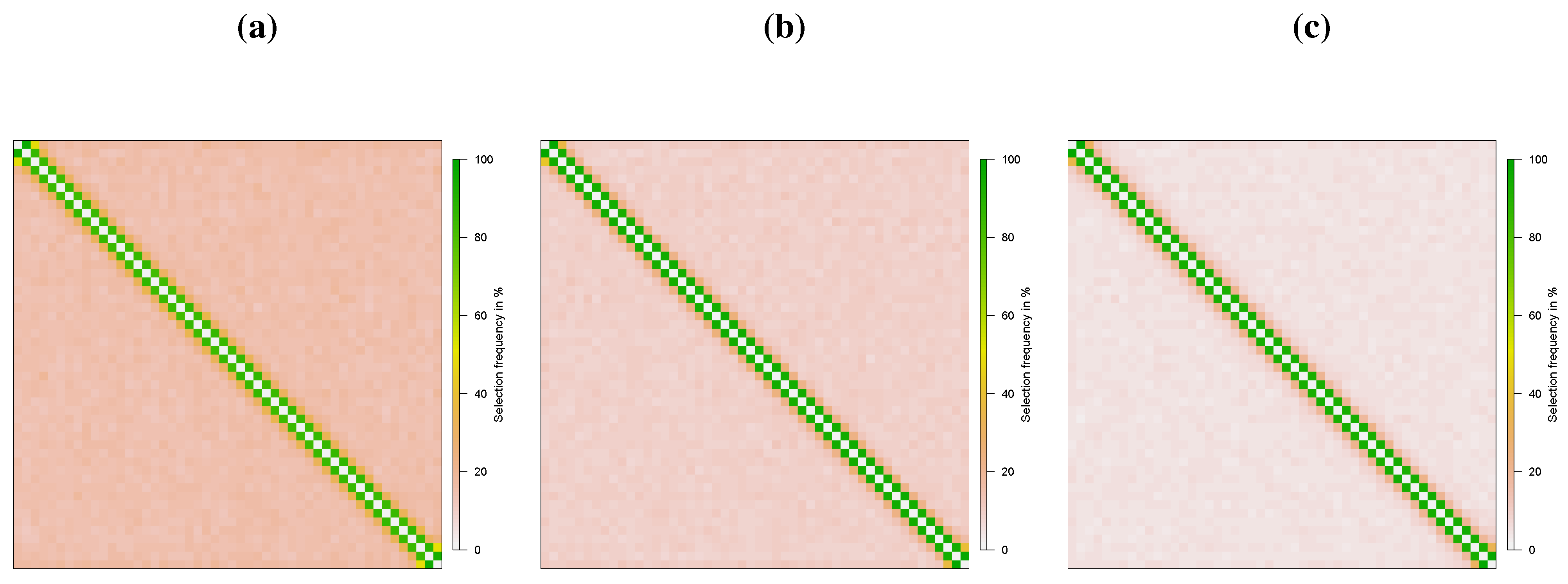
Figure 2 shows how often each $w_{ij}$ is identified as being non-zero by the estimators for $n=T=50$. It can be seen that the two-step procedures successfully recover the spatial structure in (4.2). Note that weights to the left of the sub-diagonal and to the right of the super-diagonal (i.e., $w_{13},w_{24},w_{31},\dots ,$etc.) are falsely selected slightly more often relative to other weights. This is likely due to indirect effects, resulting in spatial spillage. For example, $w_{13}$ is selected slightly more often relative to other zero elements as $y_{3t}$ affects $y_{1t}$ through $y_{2t}$.

Figure 2. Recovery of Spatial Weights Matrix (N = 50, T = 50): Specification 1. (a) Two-step Lasso; (b) Two-step post-Lasso; (c) Two-step post-Lasso with $\tau =0.05$.

Figure 2. Recovery of Spatial Weights Matrix (N = 50, T = 50): Specification 1. (a) Two-step Lasso; (b) Two-step post-Lasso; (c) Two-step post-Lasso with $\tau =0.05$.

4.2. Specification 2

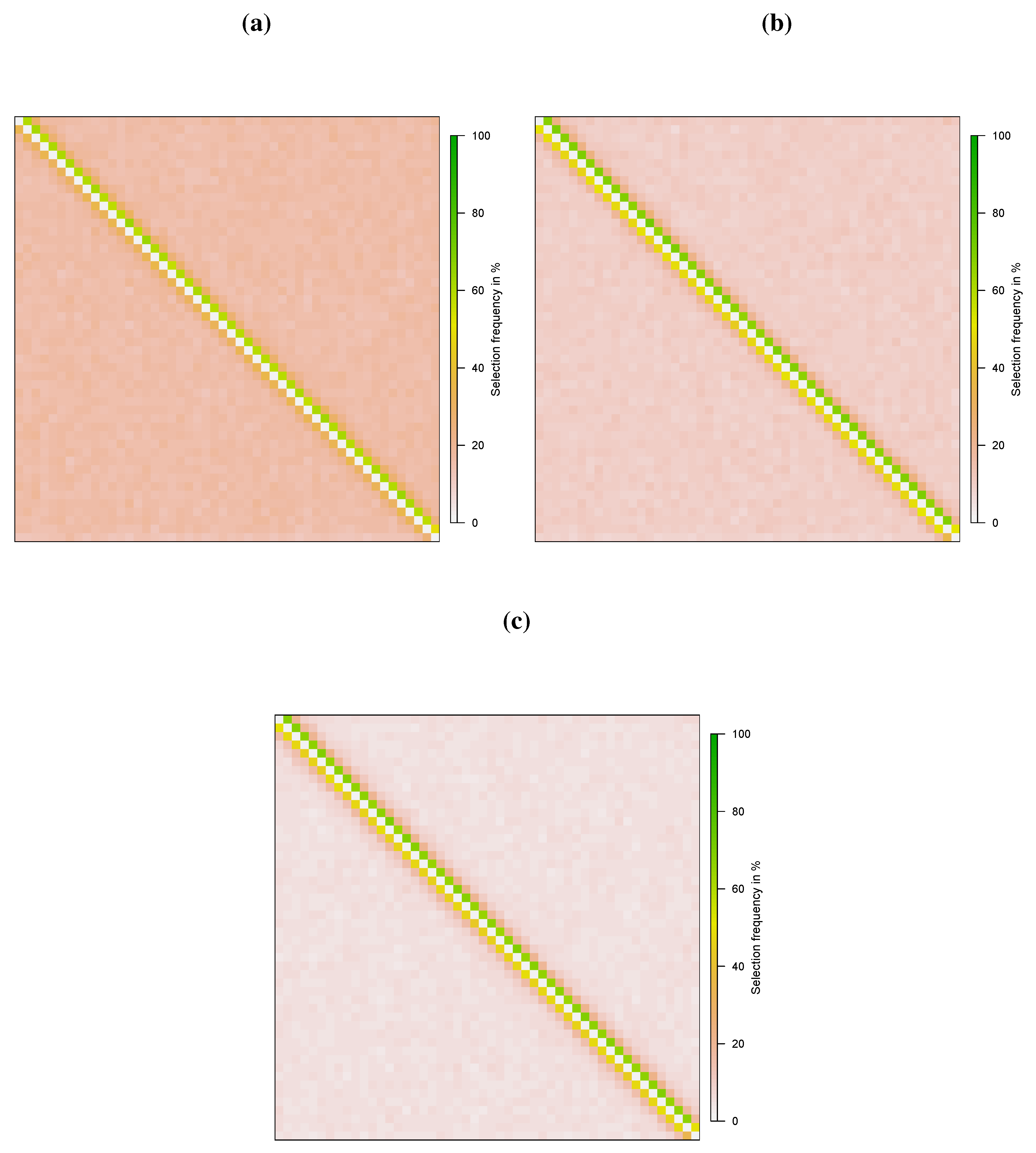
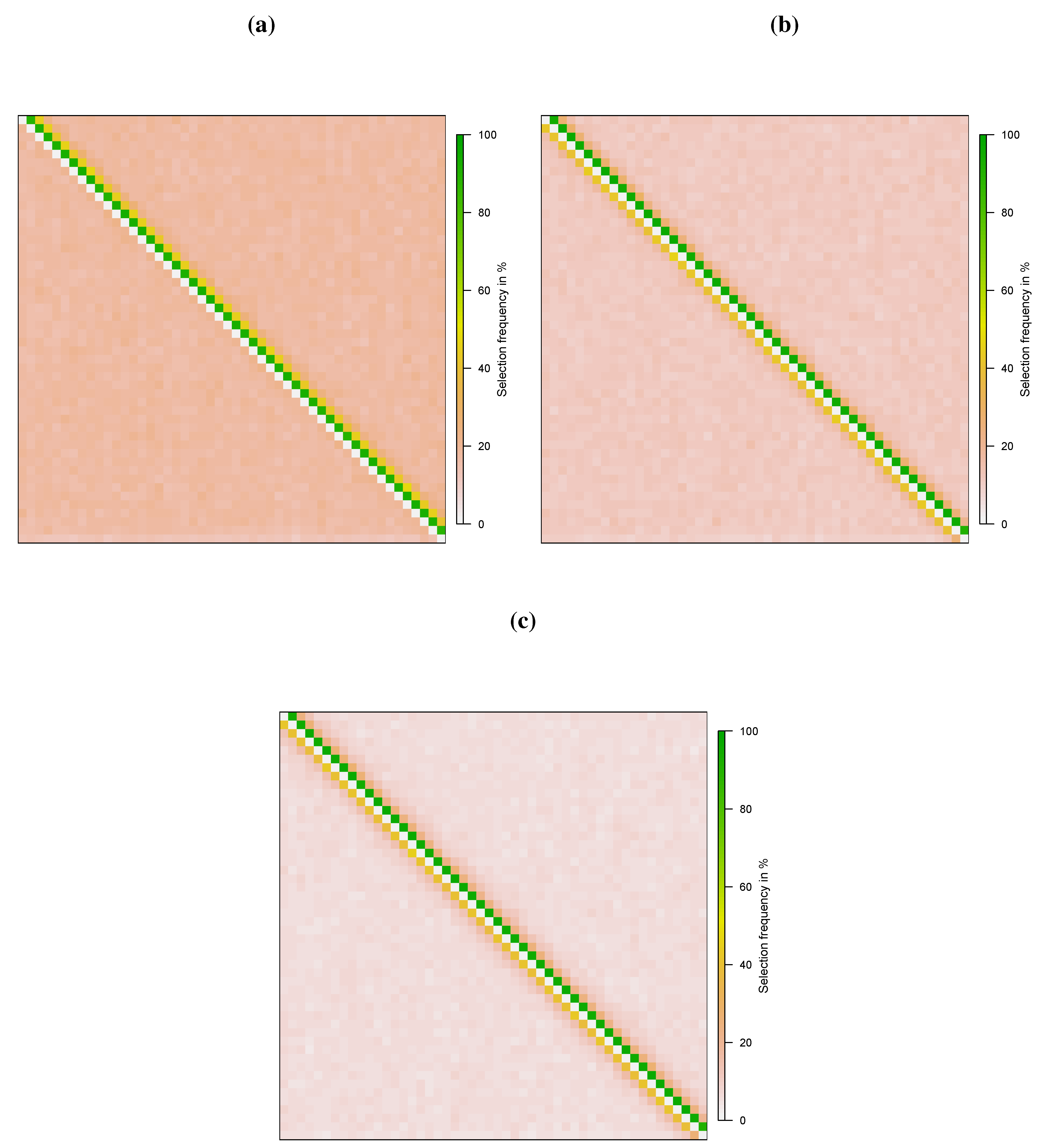
As expected, the performance under specification 2 is not as satisfactory as for specification 1. Table 2 shows that false negative rate and bias decrease in T for all three Lasso-based estimators. As in specification 1, the two-step post-Lasso outperforms the two-step Lasso in terms of the false negative rate. The thresholded Lasso mainly differs from the two-step post-Lasso in that the false positive rate is lower. Figure 3 and Figure 4 show the selection frequency for $n=T=50$ and $n=50,T=500$. For $T=50$, it can clearly be seen that the elements in the sub-diagonal are selected more often relative to other non-zero elements, stressing the difficulty of identifying the direction of the effects in small samples. This problem reduces with T and is negligible for $T=500$, see Figure 4.

Figure 3. Recovery of Spatial Weights Matrix (N = 50, T = 50): Specification 2. (a) Two-step Lasso; (b) Two-step post-Lasso; (c) Two-step post-Lasso with $\tau =0.05$.

Figure 3. Recovery of Spatial Weights Matrix (N = 50, T = 50): Specification 2. (a) Two-step Lasso; (b) Two-step post-Lasso; (c) Two-step post-Lasso with $\tau =0.05$.

Figure 4. Recovery of Spatial Weights Matrix (N = 50, T = 50): Specification 2. (a) Two-step Lasso; (b) Two-step post-Lasso; (c) Two-step post-Lasso with $\tau =0.05$.

Figure 4. Recovery of Spatial Weights Matrix (N = 50, T = 50): Specification 2. (a) Two-step Lasso; (b) Two-step post-Lasso; (c) Two-step post-Lasso with $\tau =0.05$.

Overall, the two-step Lasso performs well in recovering the network structure, even for the more challenging specification 2. However, we observe that the two-step Lasso selects too many spatial lags in small samples, although the performance improves substantially with T in terms of bias and false negative rate. The two-step post-Lasso outperforms the two-step Lasso in terms of bias and selection performance.

5. Conclusions

The identification of interaction effects is crucial for the understanding of how individuals, firms and regions interact. However, to date there is still a lack of methods that allow the estimation of interaction effects, particularly when the spatial dimension is large. Thus, most applied spatial econometric research usesad hoc specifications to incorporate interaction effects. The lack of estimation strategies may also explain why interaction effects in socio-economic processes are often ignored.

We propose a two-step procedure based on the Lasso estimator that accounts for reverse causality and allows estimating interaction effects between units in a spatial autoregressive panel model without requiring any prior knowledge about the network structure. The identifying assumption is sparsity. The two-step estimator can be implemented based on fast algorithms available for the Lasso estimator; e.g., [50]. The estimation methodology is attractive for applied research as the Lasso estimator also serves as a model selector and, hence, is relatively robust to misspecification.

We have derived convergence rates for a general two-step Lasso estimator which allows for the number of endogenous regressors and the number of instruments to be larger than the sample size. We then applied the two-step estimator to the spatial autoregressive panel model. Monte Carlo results confirm that the estimation method recovers the structure of the spatial weights matrix, even if T is as small as 50–100. However, our Monte Carlo results show a tendency for over-selection of spatial weights. The two-step post-Lasso estimator, which in each step applies OLS to the model selected by the Lasso, outperforms the two-step Lasso in terms of bias, false positive and false negative rate.

The use of the two-step Lasso raises several issues shared with other Lasso-type estimators. Controlling uncertainty and conducting inference in the Lasso is challenging and remains an area of ongoing research. Recent contributions include a Lasso significance tests due to Lockhart et al. [51] and the sample splitting approaches proposed by Wasserman and Roeder [52] and Meinshausen et al. [53] which allow for controlling the false discovery rate. Earlier seminal work on the asymptotic distribution of shrinkage estimators include Fan and Li [54] and Knight and Fu [55]. The former introduces the SCAD penalty. In addition, the choice of an optimal penalty level is an important issue. Penalized estimators typically select the penalty level oriented towards optimizing predictive performance, which may not be appropriate if the purpose is structure recovery. The optimal penalty used here is not based on cross-validation or other model selection criteria commonly employed and is therefore not directly subject to this criticism. Specifically, we follow Bickel et al. [27] and Belloni et al. [30] in choosing the smallest penalty level that dominates the noise of the problem. Our Monte Carlo results show that the proposed method works quite well in the structure discovery context.

This work suggests several lines of future research. First, given that the two-step post-Lasso outperforms the two-step Lasso, formal results for the two-step post-Lasso are required. Second, the methodology can be extended to the square-root Lasso and square-root post-Lasso. The main advantage of the square-root Lasso is that the optimal penalty level does not depend on the unknown error variance [56,57]. Hence, further performance improvements seem possible. Third, instead of relying on a two-step Lasso estimation method, an alternative estimation strategy may be based on the recent work by Fan and Liao [40] or Gautier and Tsybakov [38] who allow for endogeneity in high dimensions. These one-step procedures potentially facilitate accounting for uncertainty in model selection and estimation. These ideas are retained for future work.

References

- G. Arbia, and B. Fingleton. “New spatial econometric techniques and applications in regional science.” Papers Reg. Sci. 87 (2008): 311–317. [Google Scholar]
- R. Harris, J. Moffat, and V. Kravtsova. “In search of ‘W’.” Spat. Econ. Anal. 6 (2011): 249–270. [Google Scholar]
- L. Corrado, and B. Fingleton. “Where is the economics in spatial econometrics? ” Reg. Sci. 52 (2012): 210–239. [Google Scholar]
- J. Pinkse, M.E. Slade, and C. Brett. “Spatial price competition: A semiparametric approach.” Econometrica 70 (2002): 1111–1153. [Google Scholar]
- A. Bhattacharjee, and C. Jensen-Butler. “Estimation of the spatial weights matrix under structural constraints.” Reg. Sci. Urban Econ. 43 (2013): 617–634. [Google Scholar]
- M. Beenstock, and D. Felsenstein. “Nonparametric estimation of the spatial connectivity matrix using spatial panel data.” Geogr. Anal. 44 (2012): 386–397. [Google Scholar]
- A. Bhattacharjee, and S. Holly. “Structural interactions in spatial panels.” Empir. Econ. 40 (2011): 69–94. [Google Scholar]
- A. Bhattacharjee, and S. Holly. “Understanding interactions in social networks and committees.” Spat. Econ. Anal. 8 (2013): 23–53. [Google Scholar]
- N. Bailey, S. Holly, and M.H. Pesaran. “A two stage approach to spatiotemporal analysis with strong and weak cross-sectional dependence.” J. Appl. Econome., 2014, in press. [Google Scholar]
- H.C. Huang, N.J. Hsu, D.M. Theobald, and F.J. Breidt. “Spatial Lasso with applications to GIS model selection.” J. Comput. Graph. Statist. 19 (2010): 963–983. [Google Scholar]
- D.C. Wheeler. “Simultaneous coefficient penalization and model selection in geographically weighted regression: The geographically weighted lasso.” Environ. Plan. A 41 (2009): 722–742. [Google Scholar]
- H. Seya, D. Murakami, M. Tsutsumi, and Y. Yamagata. “Application of Lasso to the eigenvector selection problem in eigenvector-based spatial filtering.” Geogr. Anal., 2014. [Google Scholar] [CrossRef]
- E. Manresa. Madrid, Spain: CEMFI. “Estimating the structure of social interactions using panel data.” 2014, Unpublished work. [Google Scholar]
- P.C. Souza. London, UK: Department of Statistics, London School of Economics and Political Science. “Estimating networks: Lasso for spatial weights.” 2012, Unpublished work. [Google Scholar]
- C. Lam, and P.C. Souza. London, UK: Department of Statistics, London School of Economics and Political Science. “Regularization for spatial panel time series using adaptive Lasso.” 2013, Unpublished work. [Google Scholar]
- A.D. Cliff, and J.K. Ord. Spatial Autocorrelation: Monographs in Spatial and Environmental Systems Analysis. London, UK: Pion Ltd., 1973. [Google Scholar]
- L. Anselin. Spatial Econometrics: Methods and Models. New York, NY, USA: Springer, 1988. [Google Scholar]
- M. Kapoor, H.H. Kelejian, and I.R. Prucha. “Panel data models with spatially correlated error components.” J. Econom. 140 (2007): 97–130. [Google Scholar]
- L.F. Lee, and J. Yu. “Some recent developments in spatial panel data models.” Reg. Sci. Urban Econ. 40 (2010): 255–271. [Google Scholar]
- L.F. Lee, and J. Yu. “Estimation of spatial autoregressive panel data models with fixed effects.” J. Econom. 154 (2010): 165–185. [Google Scholar]
- L.F. Lee, and J. Yu. “Efficient GMM estimation of spatial dynamic panel data models with fixed effects.” J. Econom. 180 (2014): 174–197. [Google Scholar]
- J. Mutl, and M. Pfaffermayr. “The Hausman test in a Cliff and Ord panel model.” Econom. J. 14 (2011): 48–76. [Google Scholar]
- J. Elhorst. Spatial Econometrics: From Cross-Sectional Data to Spatial Panels. New York, NY, USA: Springer, 2014. [Google Scholar]
- R. Tibshirani. “Regression shrinkage and selection via the Lasso.” J. R. Stat. Soc. Ser. B (Methodological) 58 (1996): 267–288. [Google Scholar]
- H. Akaike. “A new look at the statistical model identification.” IEEE Trans. Autom. Control 19 (1974): 716–723. [Google Scholar]
- G. Schwarz. “Estimating the dimension of a model.” Ann. Stat. 6 (1978): 461–464. [Google Scholar]
- P.J. Bickel, Y. Ritov, and A.B. Tsybakov. “Simultaneous analysis of Lasso and Dantzig selector.” Ann. Stat. 37 (2009): 1705–1732. [Google Scholar]
- P. Bühlmann, and S. van de Geer. Statistics for High-Dimensional Data. New York, NY, USA: Springer, 2011. [Google Scholar]
- P. Zhao, and B. Yu. “On model selection consistency of Lasso.” J. Mach. Learn. Res. 7 (2006): 2541–2563. [Google Scholar]
- A. Belloni, D. Chen, V. Chernozhukov, and C. Hansen. “Sparse models and methods for optimal instruments with an application to eminent domain.” Econometrica 80 (2012): 2369–2429. [Google Scholar]
- A. Belloni, and V. Chernozhukov. “Least squares after model selection in high-dimensional sparse models.” Bernoulli 19 (2013): 521–547. [Google Scholar]
- F. Bunea, A. Tsybakov, and M. Wegkamp. “Sparsity oracle inequalities for the Lasso.” Electron. J. Stat. 1 (2007): 169–194. [Google Scholar]
- M.J. Wainwright. “Sharp thresholds for high-dimensional and noisy sparsity recovery using L1-constrained quadratic programming.” IEEE Trans. Inf. Theor. 55 (2009): 2183–2202. [Google Scholar]
- S. Van de Geer. “High-dimensional generalized linear models and the Lasso.” Ann. Stat. 36 (2008): 614–645. [Google Scholar]
- N. Meinshausen, and B. Yu. “Lasso-type recovery of sparse representations for high-dimensional data.” Ann. Stat. 37 (2009): 246–270. [Google Scholar]
- M.H. Pesaran. “Estimation and inference in large heterogeneous panels with a multifactor error structure.” Econometrica 74 (2006): 967–1012. [Google Scholar]
- M.H. Pesaran, and E. Tosetti. “Large panels with common factors and spatial correlation.” J. Econom. 161 (2011): 182–202. [Google Scholar]
- E. Gautier, and A.B. Tsybakov. Toulouse, France: Toulouse School of Economics. “High-dimensional instrumental variables regression and confidence sets.” 2014, Unpublished work. [Google Scholar]
- E. Candes, and T. Tao. “The Dantzig selector: Statistical estimation when p is much larger than n.” Ann. Stat. 35 (2007): 2313–2351. [Google Scholar]
- J. Fan, and Y. Liao. “Endogeneity in high dimensions.” Ann. Stat. 42 (2014): 872–917. [Google Scholar]
- M. Caner. “Lasso-type Gmm estimator.” Econom. Theor. 25 (2009): 270–290. [Google Scholar]
- W. Lin, R. Feng, and H. Li. “Regularization methods for high-dimensional instrumental variables regression with an application to genetical genomics.” J. Am. Stat. Assoc., 2014. [Google Scholar] [CrossRef]
- A. Belloni, and V. Chernozhukov. “High dimensional sparse econometric models: An introduction.” In Inverse Problems and High-Dimensional Estimation SE - 3. Edited by P. Alquier, E. Gautier and G. Stoltz. Berlin/ Heidelberg, Germany: Springer, 2011, pp. 121–156. [Google Scholar]
- B.Y. Jing, Q.M. Shao, and Q. Wang. “Self-normalized Cramér-type large deviations for independent random variables.” Ann. Probab. 31 (2003): 2167–2215. [Google Scholar]
- A. Belloni, V. Chernozhukov, and C. Hansen. “Inference on treatment effects after selection among high-dimensional controls.” Rev. Econ. Stud. 81 (2014): 608–650. [Google Scholar]
- S. Van de Geer, and P. Bühlmann. “On the conditions used to prove oracle results for the Lasso.” Electron. J. Stat. 3 (2009): 1360–1392. [Google Scholar]
- G. Raskutti, M.J. Wainwright, and B. Yu. “Restricted eigenvalue properties for correlated Gaussian designs.” J. Mach. Learn. Res. 11 (2010): 2241–2259. [Google Scholar]
- H.H. Kelejian, and I.R. Prucha. “A generalized spatial two-stage least squares procedure for estimating a spatial autoregressive model with autoregressive disturbances.” J. Real Estate Financ. Econ. 17 (1998): 99–121. [Google Scholar]
- H.H. Kelejian, and I.R. Prucha. “A generalized moments estimator for the autoregressive parameter in a spatial model.” Int. Econ. Rev. 40 (1999): 509–533. [Google Scholar]
- J. Friedman, T. Hastie, and R. Tibshirani. “Regularization paths for generalized linear models via coordinate descent.” J. Stat. Softw. 33 (2010): 1–22. [Google Scholar]
- R. Lockhart, J. Taylor, R.J. Tibshirani, and R. Tibshirani. “A significance test for the Lasso.” Ann. Stat. 42 (2014): 413–468. [Google Scholar]
- L. Wasserman, and K. Roeder. “High-dimensional variable selection.” Ann. Statist. 37 (2009): 2178–2201. [Google Scholar]
- N. Meinshausen, L. Meier, and P. Bühlmann. “p-Values for high-dimensional regression.” J. Am. Statist. Assoc. 104 (2009): 1671–1681. [Google Scholar]
- J. Fan, and R. Li. “Variable selection via nonconcave penalized likelihood and its oracle properties.” J. Am. Stat. Assoc. 96 (2001): 1348–1360. [Google Scholar]
- K. Knight, and W. Fu. “Asymptotics for Lasso-type estimators.” Ann. Stat. 28 (2000): 1356–1378. [Google Scholar]
- A. Belloni, V. Chernozhukov, and L. Wang. “Square-root lasso: Pivotal recovery of sparse signals via conic programming.” Biometrika 98 (2011): 791–806. [Google Scholar]
- A. Belloni, V. Chernozhukov, and L. Wang. “Pivotal estimation via square-root Lasso in nonparametric regression.” Ann. Stat. 42 (2014): 757–788. [Google Scholar]
© 2015 by the authors; licensee MDPI, Basel, Switzerland. This article is an open access article distributed under the terms and conditions of the Creative Commons Attribution license ( http://creativecommons.org/licenses/by/4.0/).
Share and Cite
MDPI and ACS Style
Ahrens, A.; Bhattacharjee, A. Two-Step Lasso Estimation of the Spatial Weights Matrix. Econometrics 2015, 3, 128-155. https://doi.org/10.3390/econometrics3010128
AMA Style
Ahrens A, Bhattacharjee A. Two-Step Lasso Estimation of the Spatial Weights Matrix. Econometrics. 2015; 3(1):128-155. https://doi.org/10.3390/econometrics3010128
Chicago/Turabian StyleAhrens, Achim, and Arnab Bhattacharjee. 2015. "Two-Step Lasso Estimation of the Spatial Weights Matrix" Econometrics 3, no. 1: 128-155. https://doi.org/10.3390/econometrics3010128