Article

Continuous and Jump Betas: Implications for Portfolio Diversification

1
Tasmanian School of Business and Economics, University of Tasmania, Hobart TAS 7001, Australia
2
Discipline of Finance, Business School, University of Technology Sydney, Sydney NSW 2007, Australia
3
Department of Economics, Faculty of Business and Law, Deakin University, Burwood VIC 3125, Australia
*
Author to whom correspondence should be addressed.
Econometrics 2016, 4(2), 27; https://doi.org/10.3390/econometrics4020027
Submission received: 29 February 2016 / Revised: 18 May 2016 / Accepted: 25 May 2016 / Published: 1 June 2016
(This article belongs to the Special Issue Financial High-Frequency Data)

Abstract

:
Using high-frequency data, we decompose the time-varying beta for stocks into beta for continuous systematic risk and beta for discontinuous systematic risk. Estimated discontinuous betas for S&P500 constituents between 2003 and 2011 generally exceed the corresponding continuous betas. We demonstrate how continuous and discontinuous betas decrease with portfolio diversification. Using an equiweighted broad market index, we assess the speed of convergence of continuous and discontinuous betas in portfolios of stocks as the number of holdings increase. We show that discontinuous risk dissipates faster with fewer stocks in a portfolio compared to its continuous counterpart.

1. Introduction

The quest for the optimal portfolio size that reduces diversifiable risk has been an integral part of the portfolio choice literature since Markowitz [1,2]. The concept of diversification is simple; the level of return variability falls as the number of holdings in a portfolio increases. This is true for any coherent measure of risk (e.g., [3,4]). Furthermore, as risk decreases with an increase in the number of holdings, the average return of a portfolio is unaffected, improving the risk-return trade-off. The investor may be better off holding a large number of low-quality stocks than a smaller number of high-quality stocks.
A wide range of risk measures has been proposed to answer the question of optimal portfolio size.1 With the optimal number of portfolio holdings ranging from eight to 10 stocks (e.g., [5,18]) to as many as 40 to 60 stocks (e.g., [7,12,19]) to reduce most of the diversifiable risk, it is hard to discuss or compare the results in these studies since the underlying assumptions, the data (frequencies and time periods) and assumed risk measures are different. It is, nevertheless, a powerful concept to use for between-period comparison. With rare exceptions (e.g., [16,17,20]), most diversification literature focuses on a full sample period without considering the time-series dynamics of optimal portfolio size.
This paper takes advantage of high-frequency data and new econometrics tools to split risk into its continuous and discontinuous components and derive optimal portfolio size recommendations for an average investor. The existing literature only points to the potential of high-frequency data for portfolio diversification. For example, Silvapulle and Granger [21] investigate asset correlations at the tails of return distributions and discuss the possibilities for portfolio diversification. Bollerslev et al. [22] examine the relationship between jumps in individual stocks and jumps in a market index. The authors find that jumps occur more than three times as often at the individual stock level compared to jump occurrence in an aggregate equiweighted index constructed from the same stocks. This points to the fact that jumps are diversifiable. Pukthuanthong and Roll [23] consider implications of jumps for international diversification using daily data. They find that cross-country diversification is less effective if jumps are frequent, unpredictable and strongly correlated. Only recently has the optimal portfolio size question been addressed in the high-frequency domain with Alexeev and Dungey [16] finding that optimal holdings size is affected by frequency of data. The implications of jumps for portfolio size recommendations have not been investigated.
Using extensive portfolio simulation techniques, we evaluate the variability reduction of portfolio betas as the number of holdings in these portfolios increase. Although earlier literature focuses on reducing the residual risk obtained from the Capital Asset Pricing Model (CAPM) (e.g., [13,14]), the non-parametric nature of the Todorov and Bollerslev [24] estimator that we implement to separate continuous and discontinuous beta does not allow estimation of portfolio residual risk and precludes us from investigating diversification benefits for different factors separately. Instead, we analyse the spread of estimated betas in equiweighted randomly constructed portfolios of different sizes, focusing on the difference in convergence between continuous and discontinuous betas as the number of holdings in a portfolio increases.
The interpretation of the beta coefficient as a measure of risk rests upon the empirical validity of the market model, where the return on an asset is a linear function of market factors common to all assets [25]. The focus of this paper is on decomposing the market risk factor into its continuous and discontinuous components. Evidence of the existence of jumps in many financial asset classes may be found in Andersen et al. [26], Dungey et al. [27], Jacod and Todorov [28], Lahaye et al. [29] and Aït-Sahalia and Jacod [30]. Jump risk has been shown to be an important element in improving the estimation of the yield curve [31], estimates and forecasts of daily volatility [32,33,34], explaining the high equity premium [35] and optimal hedging strategies [36]. The market itself presents evidence of significant rewards for bearing non-diversifiable jump risk; for example, via the expense of short-maturity options written on the market index with strikes that are far from its current level. Investors may treat rare events somewhat differently from common, more frequent events, in devising portfolio strategies.
Large risk premia can be obtained when the representative investor treats jump and diffusive risks differently as formalised in Bates [35]. Barro [37] shows that rare economic disasters have the potential to explain the high equity premium. Patton and Verardo [38] provide empirical evidence of substantial short-term changes in betas around earnings announcements.
The time-series relation between systematic jump risk and expected stock market returns has been examined in Santa-Clara and Yan [39], while Cremers et al. [40] examine the pricing of jump risk in the cross-section of stock returns: Stocks with high sensitivities to jump risk have low expected returns. These results are statistically significant and economically important. Guo et al. [41] show that jump risk is also an important determinant of conditional equity premium even after controlling for commonly used stock market return predictors. Recent evidence suggests that discontinuous systematic risk factors are associated with positive risk premia, while continuous counterparts are not priced or exhibit negative risk premia (e.g., [42,43]). We depart from the mainstream literature on the empirical pricing of risk factors associated with continuous and jump risks and focus on its implications for portfolio diversification.
This paper is the first to investigate the stability of systematic risk in portfolios of assets and to propose the optimal number of portfolio holdings that considerably reduces the variability of portfolio betas for an average investor. We follow Todorov and Bollerslev [24] to decompose systematic risk into continuous and discontinuous (jump) components. We show that the jump risk is easier to contain (that is, fewer portfolio holdings are required to reduce portfolio risk) than the continuous risk. We find that this difference is more pronounced during less turbulent times in contrast to periods of elevated market volatility when estimates of continuous and discontinuous betas are often of similar magnitudes.
The remainder of this paper is organised as follows. Section 2 describes the dataset used in the empirical analysis. Section 3 introduces the modelling framework and parameter choices for estimating the continuous and discontinuous betas. Our empirical analysis in Section 4 includes the estimation of individual stock betas, discussion of their properties and some robustness tests. In Section 5, we turn to the selection of portfolio size and assess the implications of the two risk components for portfolio diversification. Section 6 concludes the paper.

2. Data

We investigate 501 stocks from the S&P500 index over a 9-year sample period from 2 January 2003 to 30 December 2011. This period covers the turmoil of the third quarter of 2008 associated with the bankruptcy of Lehman Brothers and rescue/intervention packages around financial firms in the US at this time. The data consist of 5-min price observations between 9:30 am and 4:00 pm eastern standard time (EST) of stocks after adjusting for mergers and acquisitions, stock splits, trading halts and bankruptcies.2 We follow current convention in using 5-min observations, see Andersen et al. [26], Lahaye et al. [29], as the choice of optimal sampling frequency for multiple asset problems is as yet an unresolved problem. In Alexeev et al. [42], we show that the Epps effect is not substantial in these data. The final sample consists of 2262 active trading days across 108 months, with 77 observations per day. Missing 5-min observations are filled with the previous observation, and during each estimation window, we draw from the population of stocks with at least 75% of non-zero 5-min returns to obtain sufficient data coverage for high-frequency analysis.
Our estimation window is a calendar month, enabling us to conduct dynamic analysis of the portfolio results with non-overlapping windows of data. The benchmark portfolio is constructed as an equally weighted portfolio of investible stocks in each estimation window; we choose this in preference to a value-weighted portfolio to avoid cases where one stock has a disproportionately high weight in the portfolio. The portfolio analysis is conducted with 12-month rolling windows to avoid interrupting the dynamics in the discontinuous beta and to consider the implications of portfolios with annual rebalancing.

3. Modeling Framework

Given a panel of N assets, the continuous-time data generating process (DGP) of an asset’s log-price p i , t is typically characterised as a semi-martingale process plus jumps, i = 1 , , N . The instantaneous return, r i , t , takes the following form:
r i , t d p i , t = b i , t d t + σ i , t d W i , t + κ i , t d μ i , t , t ( 0 , T ] ,
where b i , t and σ i , t measure the time-varying drift and spot volatility, respectively, and W i , t denotes a standard Brownian motion, i = 1 , , N . In the discontinuous component, κ i , t = p i , t - p i , t - denotes the size of the jump in the i-th asset at time t, and μ i , t is a Poisson random measure that counts the number of jump occurrences. We omit the possibly infinite jump activity for simplicity as it does not affect our model dynamics.
Denote the return on a benchmark market portfolio as r 0 , t . A standard one-factor asset pricing model representation relating r i , t to r 0 , t takes the form
r i , t = α i + β i r 0 , t + ϵ i , t , i = 1 , , N .
The β i coefficient in Equation (2) is the sensitivity of the expected return on the i-th asset to the return on the market (or systematic) factor.3 Following Todorov and Bollerslev [24], the market return r 0 , t can be represented in the same way as in Equation (1) consisting of the continuous and discontinuous components. Hence, in the presence of jumps, Equation (2) becomes
r i , t = α i + β i c σ 0 , t d W 0 , t + β i d κ 0 , t d μ 0 , t + ϵ i , t , i = 1 , , N ,
where ϵ i , t in this case contains both the idiosyncratic continuous and discontinuous components in each asset.
Equation (3) implies that the sensitivity of an asset return to the two components of systematic risk can be different, represented by β i c and β i d , respectively. Overall, systematic risk is due to either the continuous component of the market movement σ 0 , t d W 0 , t , or the discontinuous component κ 0 , t d μ 0 , t . Assuming that the continuous record of the asset returns r i , t and r 0 , t are available, β i c and β i d can be derived from (3) using covariation measures.
For any i = 0 , 1 , , N , the quadratic variation of r i , t over the time interval ( 0 , T ] is defined as
[ r i , r i ] T 2 = 0 t σ i , s 2 d s + 0 < s t κ i , s 2 .
It follows that the quadratic covariation between r i , t and r 0 , t is
[ r i , r 0 ] T 2 = β i c 0 t σ 0 , s 2 d s [ r i c , r 0 c ] T 2 + β i d 0 < s t κ 0 , s 2 [ r i d , r 0 d ] T 2 .
The first term in Equation (5), [ r i c , r 0 c ] T 2 , captures the covariation in the continuous components of r i , t and r 0 , t , whereas the second term represents the discontinuous covariation. For the continuous beta,
β i c = [ r i c , r 0 c ] T 2 [ r 0 c , r 0 c ] T 2 , i = 1 , , N ,
and
[ r i d , r 0 d ] T 2 τ = ( β i d ) τ 0 < s t κ 0 , s 2 τ = ( β i d ) τ [ r 0 d , r 0 d ] T 2 τ , τ 1 ,
for the discontinuous beta.4 Equation (6) and Equation (7) provide the basis for constructing discrete-sample estimators of β i c and β i d .

3.1. The Estimators in Discrete Time

Empirical applications do not have the luxury of continuously recorded asset prices and returns. Instead, we assume that they are observed at every Δ time interval, from 0 , Δ , 2 Δ , , to T / Δ · Δ . Hence, there are T / Δ interval returns within ( 0 , T ] , which are denoted by
r i , j = p i , j - p i , j - 1 , i = 0 , 1 , , N , j = 1 , , T / Δ .
The consistent estimators for β i c and β i d given by Todorov and Bollerslev [24] are constructed as follows: Let r j = r 0 , j , r 1 , j , , r N , j be the ( N + 1 ) × 1 vector of the observed returns, j = 1 , , T / Δ . The sample counterpart of (6) is constructed using truncated realised covariations,
β ^ i c = j = 1 T / Δ r i , j r 0 , j 1 { | r j | θ } j = 1 T / Δ r 0 , j 2 1 { | r j | θ } , i = 1 , , N ,
where θ = ( a 0 Δ ϖ , a 1 Δ ϖ , , a N Δ ϖ ) , ϖ ( 0 , 1 2 ) , a i 0 , and 1 denotes the indicator function. The truncated realised covariation j = 1 T / Δ r i , j r 0 , j 1 { | r j | θ } extends the univariate measure first proposed by Mancini [48] and provides a consistent estimator of [ r i c , r 0 c ] T 2 as Δ 0 . The constant a i in the truncation threshold is usually set as a function of the estimated volatility of the i-th asset in order to take into account the time-varying volatility. Todorov and Bollerslev [24] show that β ^ i c given by (9) converges to the true value as Δ 0 .
The discrete-time estimator of β i d utilises higher power covariations,
β ^ i d = sign j = 1 T / Δ sign { r i , j r 0 , j } | r i , j r 0 , j | τ × j = 1 T / Δ sign { r i , j r 0 , j } | r i , j r 0 , j | τ j = 1 T / Δ r 0 , j 2 τ 1 τ ,
where the power τ is restricted to τ 2 so that the continuous price movements become negligible asymptotically and only large returns are retained. An alternative estimator of the discontinuous beta relies on the truncation technique. Instead of taking the “small” returns as in (9), it collects the complement set of { | r j | θ } and inserts this in Equation (10). Both estimators are consistent and asymptotically equivalent (see [24] for more details).5 However, Theorem 1 in Todorov and Bollerslev [24] suggests that the convergence in probability of β ^ i d only holds if there is at least one jump in the market portfolio r 0 , t over the interval ( 0 , T ] . Therefore, in order to calculate β ^ i d , we first need to test for the existence of jumps in the market portfolio.

3.2. Testing for Jumps

There are several well-developed jump tests in the existing literature (see, for example [49,50,51,52] among others), and for a review see Dumitru and Urga [53]. Following Todorov and Bollerslev [24], we use the test statistic proposed by Barndorff-Nielsen and Shephard [50] to detect jumps in the market portfolio.6
Denote the realised volatility of r 0 , t at sampling frequency Δ as
R V 0 , T = j = 1 T / Δ r 0 , j 2 P [ r 0 , r 0 ] T 2 as Δ 0 ,
where [ r 0 , r 0 ] T 2 is the quadratic variation as in Equation (4). Barndorff-Nielsen and Shephard [56] propose a consistent estimator of the continuous quadratic variation, referred to as the bipower variation of the form
B V 0 , T = j = 1 T / Δ - 1 | r 0 , j | | r 0 , j + 1 | P μ 1 2 0 T σ s 2 d s as Δ 0 ,
where μ 1 = 2 / π . It follows immediately that the difference between R V T and μ 1 - 2 B V T could consistently estimate the jump variation of the market portfolio. Hence, combining Equation (4), Equation (11) and Equation (12) leads to the result that
R V 0 , T - μ 1 - 2 B V 0 , T P 0 < s T κ s 2 .
The feasible test statistic is given by
J ^ 0 , T = 1 Δ · 1 ϕ · max 1 / T , D V 0 , T / B V 0 , T 2 μ 1 - 2 · B V 0 , T - R V 0 , T R V 0 , T ,
where ϕ = π 2 / 4 + π - 5 and D V 0 is the realised quadpower variation
D V 0 , T = 1 Δ j = 1 [ T / Δ ] - 3 | r 0 , j | | r 0 , j + 1 | | r 0 , j + 2 | | r 0 , j + 3 | .
The test statistic J ^ 0 , T has an asymptotic standard normal distribution as Δ 0 . In practice, given a fixed time interval ( 0 , T ] , our estimation starts with a jump test in the market index. If J ^ 0 , T exceeds the critical value at the desired level of significance, we proceed to estimate both the continuous and discontinuous betas as presented in (9) and (10). Otherwise, we calculate only the continuous beta for the given time period as the discontinuous beta is not identified.

3.3. Choices of Parameter Values

Many existing jump tests suffer from severe size distortion whereby too many jumps are detected (e.g., [57]). One remedy is to use extremely conservative critical values. Therefore, we use 0.1% level of significance in testing for jumps in the market portfolio. We first normalise each estimation window—one calendar month to be one unit in time, thus setting Δ to be the reciprocal of the number of observations in each month. We follow Todorov and Bollerslev [24] and set ϖ = 0 . 49 , letting a i vary amongst individual stocks. Denoting the bipower variation of the i-th stock over the time interval ( 0 , T ] by B V i , T , we set a i = 3 B V i , T , i = 0 , 1 , , N . Intuitively, this means that returns within three standard deviations are considered as generated by the continuous Brownian component, where the time-varying spot volatility is estimated by the square root of bipower variation.
Recall that, when calculating β ^ i c in Equation (9), only those observations that satisfy | r j | θ are used. As the total number of stocks considered here, N, is quite high, this condition can be rather restrictive for all N stock returns to be bounded below the threshold. We conduct robustness tests using different truncation thresholds to examine whether the estimated β i c is robust to less (or more) restrictive truncation levels in Section 4.2. Finally, the value of τ in Equation (10) is set to τ = 2 in accordance with Todorov and Bollerslev [24].

4. Estimated Betas

We detect jumps in our equally weighted market portfolio, which plays the role of r 0 in the estimation of β c and β d , on 161 out of 2262 trading days, using the statistic J ^ 0 , T given in Equation (14); that is 7.1% of all trading days. This corresponds to 82 jump months (months containing at least one jump day) out of the total 108 months in the sample. These results provide us with the days on which to conduct analysis of jump betas for portfolios. The proportion of jump days is consistent with previous empirical studies on US stock markets. For example, Andersen et al. [26] use the same ratio test on the S&P500 index from December 1986 to June 1999 and find 7.6% significant jump days.

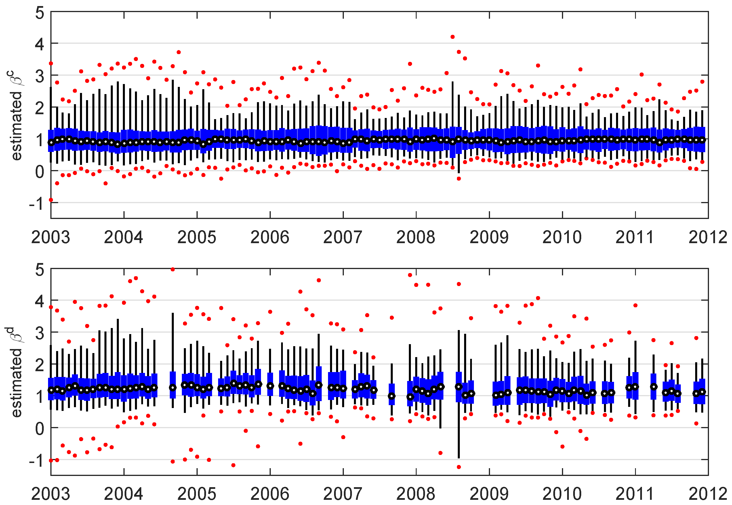
4.1. Summary Statistics of the Estimated Betas

Our continuous and jump risk betas are directly scale comparable. We find that for individual stocks drawn from the S&P500 index the continuous beta is lower than the jump beta nearly 90% of the time, indicating that most of the stocks are more sensitive to the sudden arrival of new information than to general market volatility. On average, for individual stocks, jump betas are 38% higher than continuous betas. This is more than twice the increase in betas estimated around earnings announcements in Patton and Verardo [38]. As jumps are an indicator of new information arrival, and Patton and Verardo [38] find that earnings announcements are used as a learning mechanism to update expectations about the economy, the finding that the jump beta exceeds the continuous beta may imply faster updating for unexpected information arrival than previously estimated.
Neither continuous nor jump beta estimates show any obvious trend over the sample period. However, during the months of increased market volatility (e.g., September–December 2007, September–December 2008, November 2009 and May 2010), more than 30% of the stocks exhibit lower sensitivities to jump risk than to continuous risk. This result may appear counterintuitive, but in fact the explanation is straightforward. First, beta measures the sensitivity of an individual stock to one unit of risk exposure. As the magnitude of jumps, in general, is expected to be larger than the magnitude of continuous price movements, the overall impact of a jump may still be stronger. Second, crisis periods are characterised by increased market volatility. Given a particular magnitude of price discontinuity, it may be classified as a jump during a tranquil period but also reasonably fall in the category of a continuous price movement during a period of high volatility, thus shifting the impact from a jump beta to continuous beta estimate for that period. The reduction in jumps during periods of increased market volatility is consistent with the existing literature (see [58]). As a consequence, for both the cross-sectional mean and median estimates, the gap between the discontinuous and continuous beta estimates falls during the second half of our sample when the market is in distress. This can be partly explained by the high market volatility during the crisis periods. During times of high market stress, the overall market environment becomes relatively more important than unexpected news shocks to the system. The reaction to frequent unexpected news during stressed market times may become a feature of the overall market conditions.
In Figure 1, we depict the cross-sectional distributions of monthly estimates β ^ c (top panel) and β ^ d (bottom panel) across all stocks. Since our market index is an equally weighted portfolio, by construction, the mean of β ^ c is unity for every month. The jump betas are consistently higher than the continuous betas. The average impact of individual events (or news) that are sufficient to cause price discontinuities is largely contained in the range 1.1–1.5. Furthermore, Figure 1 shows that the distribution of the estimated discontinuous beta is usually more dispersed than the estimated continuous beta. This is particularly evident in the third quarter of 2008, associated with the bankruptcy of Lehman Brothers, the rescue of AIG and the Troubled Asset Relief Program (TARP) by the US government.
Alexeev et al. [42] consider different firm characteristics to explain the variability in continuous and discontinuous betas. They find that smaller stocks are more sensitive to discontinuities than their larger counterparts, and during periods of financial distress, high leverage stocks are more exposed to continuous risk. Industry effects are also apparent. Instead, in this paper, we demonstrate how continuous and discontinuous betas of randomly selected portfolios of stocks decrease with diversification.7

4.2. Robustness Analysis

Here, we investigate the robustness of the empirical results with respect to different choices of the parameter values, as well as sampling frequency and choice of jump decomposition methodology. Most of the nuisance parameters do not affect the consistency property of the estimators but will impact finite sample applications.
For monthly estimates of the βs, the value of Δ changes from one month to another because the number of observations is different. We choose an average number of observations per month and set Δ = 1 / 1613 for all calender months and calculate the monthly β ^ c and β ^ d for all stocks. There are still 82 months that contain at least one jump day using the adjusted ratio test by Barndorff-Nielsen and Shephard [50]. Both β ^ c and β ^ d are almost the same as in our previous results.
Next we consider different values for a i in the truncation threshold θ . Changing the value of a i will affect the number of observations involved in the calculation of β ^ i c ; hence, we cannot set a i too restrictively in order to retain sufficient observations to estimate (9). By setting a i = 3 B V i , we implicitly assume that price movements within three standard deviations of the Brownian component are associated with the continuous price movements; roughly 30% of the total observations are retained. Notice that in Equation (9), | r i , j | a i Δ ϖ needs to be satisfied for each i = 0 , 1 , , N . For large N, we can lose a considerable number of observations using this truncation threshold. Thus, we only examine the situations where the value of a i is reduced. Results show that the monthly estimates β ^ i c are robust to more relaxed truncation thresholds.
We now consider using different test statistics given by Barndorff-Nielsen and Shephard [50] for detecting jump days. Apart from the adjusted ratio test J ^ 0 , T , there are two other test statistics that have the same asymptotic distribution:
G ^ 0 , T = 1 Δ μ 1 - 2 · B V 0 , T - R V 0 , T ϕ μ 1 - 4 · D V 0 , T L N ( 0 , 1 ) ,
H ^ 0 , T = 1 Δ 1 ϕ · D V 0 , T / B V 0 , T 2 μ 1 - 2 · B V 0 , T - R V 0 , T R V 0 , T L N ( 0 , 1 ) .
The difference statistic, G ^ 0 , T , and the ratio statistic, H ^ 0 , T , in general, detect more jump days than the adjusted ratio statistic, J ^ 0 , T , in Equation (14). For the equally weighted portfolio, using G ^ 0 , T leads to 314 jump days contained in 98 months and using H ^ 0 , T leads to 161 jump days contained in 82 months. Most of the corresponding β ^ i d s do not alter up to one decimal place.
In addition to using different test statistics to identify jump days, there are also alternative decompositions for detecting the contribution of jumps to total realised volatility. For example, Christensen et al. [57] suggest a pre-averaging method based on higher frequency data than the equi-distant sampling method used in the current dataset. To demonstrate that this effect is unlikely to have significant impact, we plot the volatility signature plot for four of our constituent stocks as per the Christensen et al. [57] method along with that for the equi-distant data (see Figure 2). Although there may be up to 20% variation between the contributions at ultra-high frequency, such as 1-s intervals, at the 5-min interval employed here the differences are minimal. At this point, given the variety of stocks we are using, the differences in liquidity and the hand-picked nature of the dataset as described in Section 2, we have no means of determining whether ultra-high frequency 1-s data would provide a meaningful improvement in our estimates. We note that the pre-averaging approach of Jacod et al. [59] has not been widely adopted for small samples. To our knowledge, there is no comparable study for a broad range of assets used in a portfolio context as undertaken here.
Concerns about the appropriate choice of sampling frequency also suggest that one should be wary of the Epps effect; the reason that both Patton and Verardo [38] and Todorov and Bollerslev [24] use lower frequency sampling than we employ here. Robustness checks to our estimated β c and β d to 5, 10, 20 and 30 min sampling frequencies display no significant Epps effect. These results are available from the authors on request.

5. Portfolio Diversification with Betas

Investors who hold several S&P500 stocks may be rightfully concerned with the overall exposure of their portfolios to systematic continuous and discontinuous risk. While individual securities exhibit a wide range of sensitivities to both continuous and jump risks, as shown in Figure 1, a portfolio of multiple stocks may have sensitivities to these risk factors that are more concentrated and approach the asymptotic beta coefficient of 1 at differing velocities. To address this question, we construct different size portfolios of stocks and investigate how the number of stocks selected may help to reduce the variability of the overall beta of the portfolio.
We construct 1000 random equally weighted portfolios and estimate systematic continuous and discontinuous risks, β c and β d , for each of these portfolios for each month from 2003 to 2011. We assess the stability of the systematic portfolio risks as the number of stocks in the portfolio increases by analyzing the inter-percentile ranges (IPR) of the estimated beta distributions. Defined as the difference between two percentiles, the inter-percentile range is a stable measure that is robust to outliers. We use central 50% and 90% IPRs, defined as I Q R ( n ) I P R ( n ) , 75 % - 25 % = E D F ( n ) - 1 ( . 75 ) - E D F ( n ) - 1 ( . 25 ) and I P R ( n ) , 95 % - 5 % = E D F ( n ) - 1 ( . 95 ) - E D F ( n ) - 1 ( . 05 ) , where E D F ( n ) is the empirical distribution function of the estimated betas (either β c or β d ) for randomly drawn n-stock portfolios.
Panel (a) of Figure 3 depicts the typical distributions of β for the (equally weighted) portfolios as the size of the portfolio increases from one to 200 stocks ( n = 1 , , 200 ) stocks. The specific example in panel (a) is based on β c estimated using 12-month data from March 2005 to February 2006. (A similar figure exists for distributions of estimated β d but is omitted for brevity.) Since these central ranges are dependent on the particular time period analyzed, we normalise to represent a fraction of the beta range of individual securities. The normalised IQRs, or I Q R ( n ) / I Q R ( 1 ) , for both β ^ c and β ^ d are depicted in panel (b) of Figure 3 for n = 1 , , 200 . Since the market index is an equally weighted portfolio consisting of all investible stocks (as used to detect the days on which jumps occur) and is thus unique, it has I Q R ( N ) = 0 . As a result, the normalised IQRs in panel (b) of Figure 3 are bounded between 0 and 1.
Figure 3 shows that the IQR of portfolio betas decreases substantially as the number of stocks, n, in the portfolio increases. The decrease in variation of portfolio betas is substantial for smaller portfolios, eventually decaying as more securities are added to the portfolio. Using the normalised IQRs enables us to contrast the required portfolio sizes at different periods of time to achieve the same proportional reduction in the IQRs of beta for these portfolios relative to the beta spreads of individual securities. Figure 4 illustrates the required portfolio sizes to reduce the normalised I Q R ( n ) or I P R ( n ) , 95 % - 5 % by tenfold (panels (a) and (b)) and fivefold (panels (c) and (d)).8 It is evident that in the first part of the sample, prior to the crisis of 2007, the number of stocks required to reduce the IQR is considerably higher than in the more volatile periods from 2008 onwards. A reduction in the spread of a continuous risk component in the majority of portfolios by a factor of five relative to the beta spread of individual securities requires roughly twice as many stocks in the pre-crisis period than the same proportionate reduction in the spread of discontinuous systematic risk (panel (a) of Figure 4). This aspect is not evident in results based on normalised I P R ( n ) , 95 % - 5 % .
Figure 4 shows that a portfolio requires fewer stocks to achieve discontinuous systematic risk stability than continuous systematic risk stability, and this is especially evident in the pre-crisis period. In contrast, the market seems to be indifferent to the distinction between continuous and discontinuous systematic risk for diversification purposes during the period of crisis post-2007. The difference in the number of stocks required in order to achieve the same proportionate reduction in beta spreads for continuous risk has decreased substantially.

6. Conclusions

Developments in high-frequency financial econometrics have shown considerable gains in forecasting and estimating volatility for many assets, including, in particular, the benefits of including the potential for jump behaviours. This paper is the first to consider the impact of jumps on optimal portfolio size decisions and the first to separately estimate continuous and discontinuous portfolio beta and to consider the dynamics of these decisions when faced with changing market conditions over time. We find that fewer stocks are required to achieve stability in the discontinuous risk component of the portfolio than for the continuous risk component, and this is particularly evident in the pre-crisis period. During the period of turmoil in the sample, the market does not strongly differentiate between continuous and discontinuous systematic risk in terms of diversification. The number of stocks required to produce a reduction in beta during a period of stress is reduced over the number required during a low-stress period.
Jump betas for individual stocks exceed continuous betas almost 90% of the time; however, during the period of turmoil in the sample, we find that more than 30% of the stocks have lower exposure to jump risk than the continuous risk. During these times of stress, the market perceives jump risk and continuous risk as equally important. As a result, the number of stocks required to reduce the variability of the two betas is clearly separable in the non-crisis period and less so during turmoil. During the non-crisis period, the variability of portfolio betas can be reduced fivefold (tenfold) with 50–60 (120–160) stocks for the continuous beta, but the corresponding reduction in the discontinuous beta requires only half of these amounts. During periods of financial distress, the number of stocks required to achieve the same reductions in variability of the two betas is 20–30 (60–100) stocks with less apparent distinction between the two risk components.
Our future work will include the analysis of industry effects to assess the benefits of industry diversification, that is, using stratified sampling in constructing portfolios, and the impact of asymmetry. As highlighted by Ang et al. [60], extreme losses may be perceived differently by market participants than extreme gains, implying potential asymmetry in jump betas with applications for portfolio diversification based on negative versus positive jump betas. Additional work is also anticipated in this research agenda in an examination of the small sample properties of extending the non-parametric methodology of Todorov and Bollerslev [24] to new methods of detecting jump decompositions, such as those proposed in Christensen et al. [57].

Acknowledgments

We are grateful for comments from the editor and two anonymous referees of Econometrics, Torben Andersen, Eser Arisoy, Andrew Patton, George Tauchen, Viktor Todorov and participants at the 2013 Midwest Econometrics Group Meeting, Securities Industry Research Centre of Asia-Pacific (SIRCA) Young Researcher Workshop, the Auckland Finance Meeting, 2014, the China Meeting of the Econometric Society, and the Econometric Society Australasian Meeting. Mardi Dungey acknowledges funding from Australian Research Council (ARC) grant DP130100168.

Author Contributions

The three authors contributed equally to this work.

Conflicts of Interest

The authors declare no conflict of interest.
  • 1.Existing studies use standard deviation [5,6,7], mean absolute deviation [8,9], semi-variance [10], terminal wealth standard deviation [11,12], residual variance from the CAPM [13,14], mean realised dispersion [15], and realised volatility [16]. For a comprehensive list of different risk measures used in portfolio diversification, see ([17] p. 44).
  • 2.There are 900 stocks in the original dataset of stocks that have been represented on the S&P500 at any time during the sample period. We additionally delete stocks that have altered currency of trade, are over-the-counter or listed on alternative exchanges. See Dungey et al. [44] for further database details.
  • 3.Classic references in the literature are Sharpe [45], Lintner [46] and Lintner [47] among others.
  • 4.The parameter τ in (7) can be more loosely specified such that 2 τ is above the Blumenthal-Getoor index, which covers the set of { τ : τ 1 } . However, in practice, higher values of τ are usually chosen to avoid friction caused by discrete sampling. For further details, see Todorov and Bollerslev [24].
  • 5.The small sample properties of the two discrete estimators have been investigated in Alexeev et al. [42]. The authors show that the estimation bias becomes a concern only when the difference between β c and β d exceeds unity. This is not the case in the current application.
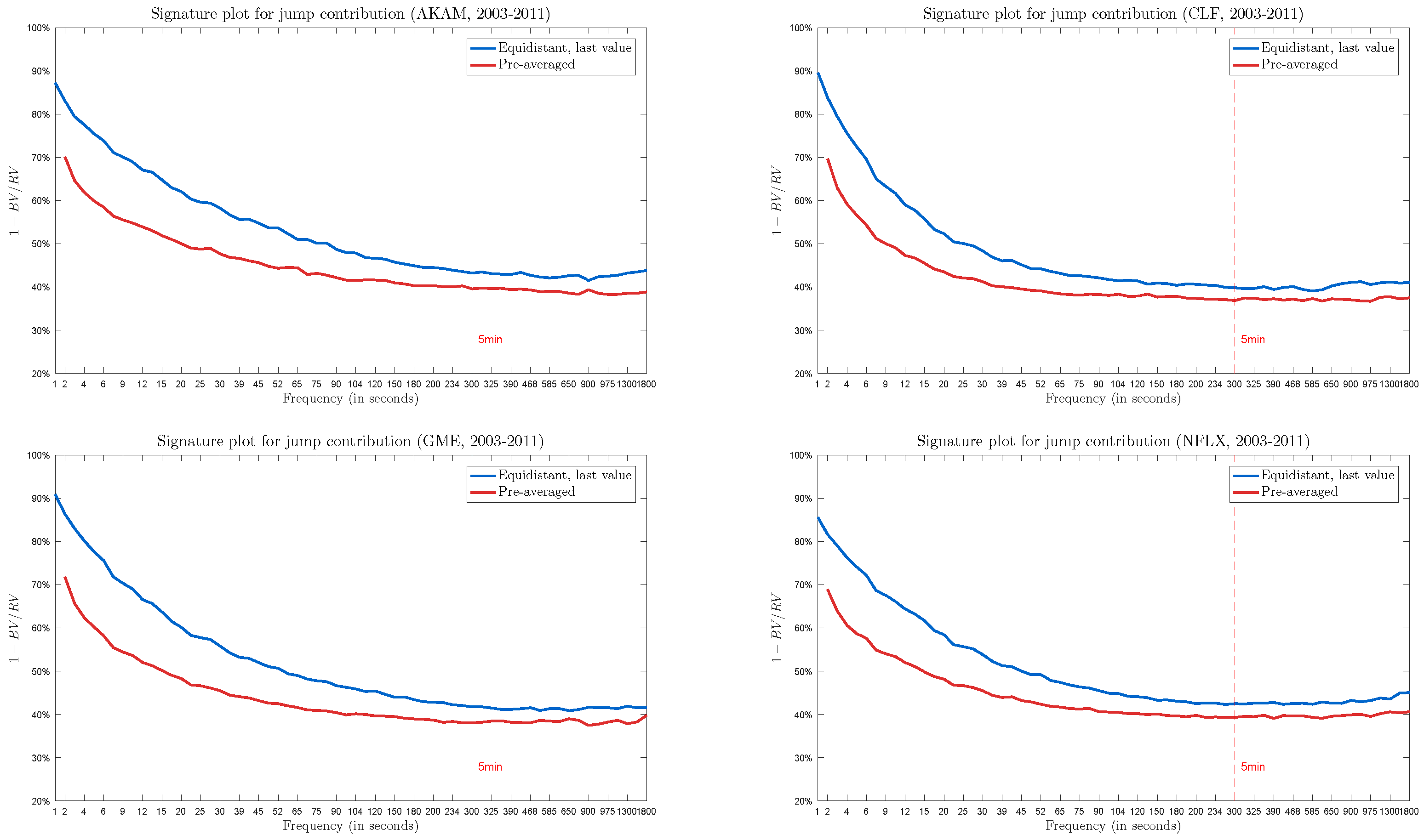
  • 6.Alternatively, if microstructure noise, nonsynchronicity and intraday volatility patterns are persistent, one could use the robust two-time scale estimator of Boudt and Zhang [54] to take these into account. The estimator is implemented using the modified Lee and Mykland [51] jump statistic proposed in Boudt et al. [55].
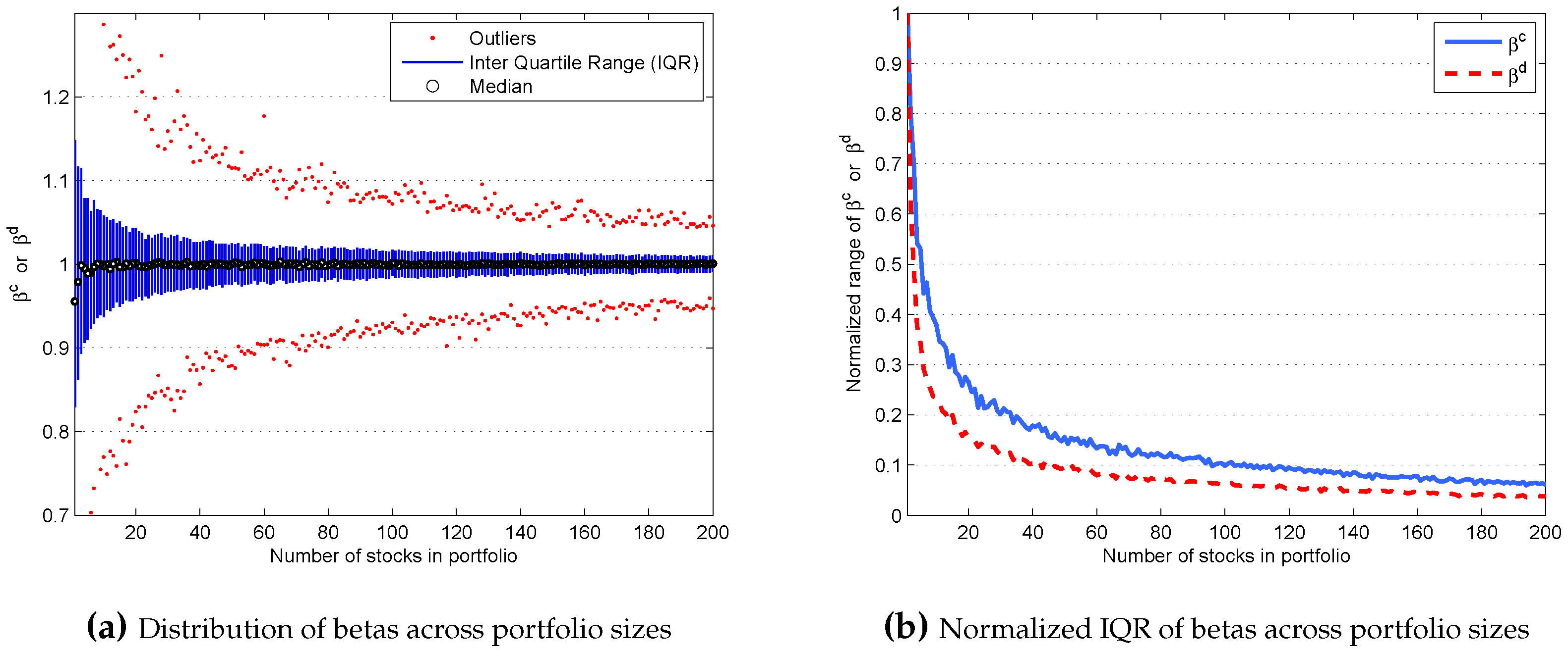
  • 7.Given the difference in variability in betas with firm characteristics, future research could explore a stratified sampling scheme to further the diversification benefits.
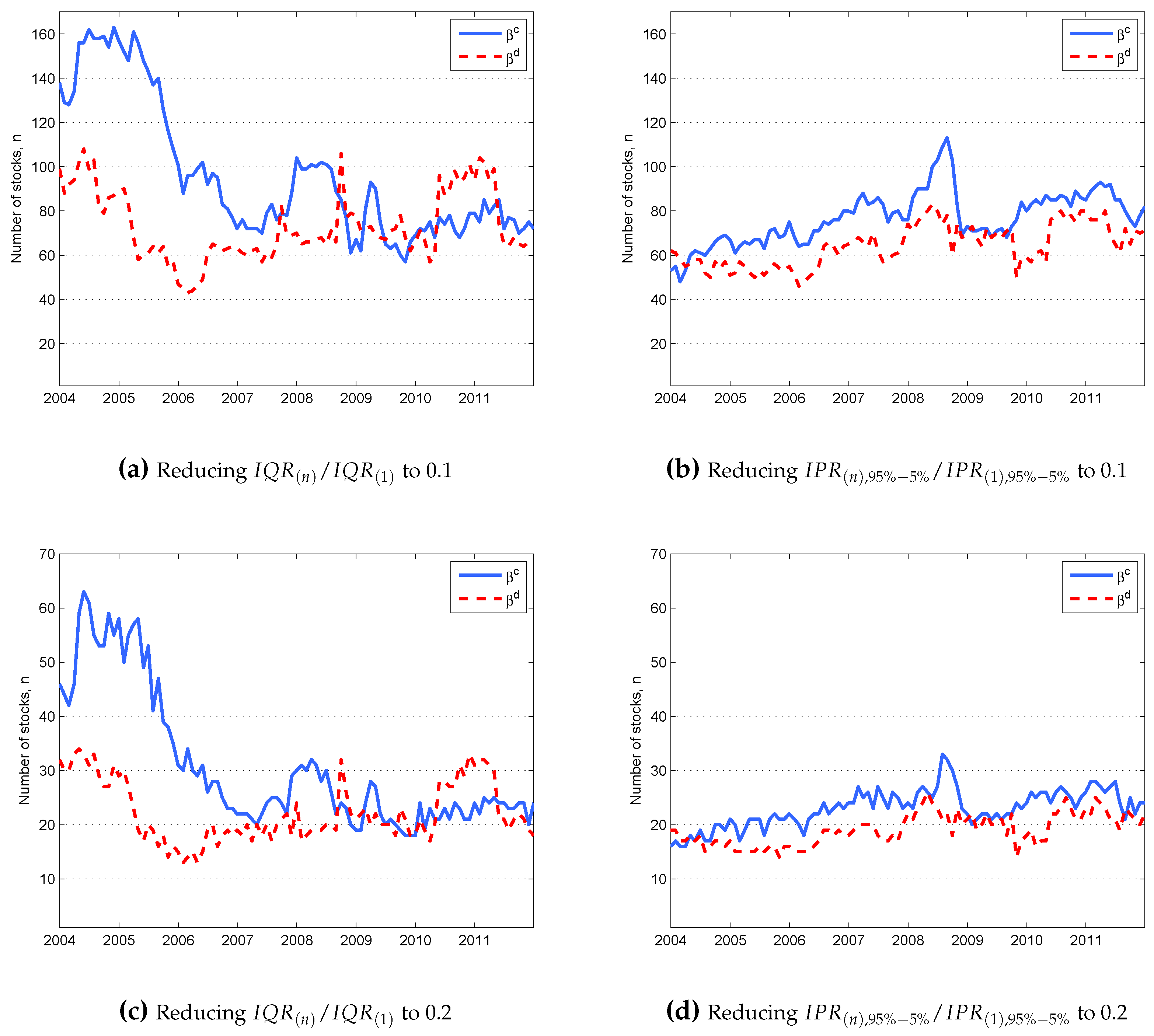
  • 8.A portfolio size resulting in a 10-fold reduction in the normalised IQR can be inferred from Figure 3b through the intersection of the blue and red curves with the horizontal line at 0.1. Figures similar to Figure 3b are constructed for each time period, and the corresponding portfolio sizes are determined from each of these figures and plotted in Figure 4a.

References

  1. H. Markowitz. “Portfolio Selection.” J. Finance 7 (1952): 77–91. [Google Scholar] [CrossRef]
  2. H. Markowitz. Portfolio Selection: Efficient Diversification of Investments. New York, NY, USA: John Wiley & Sons, 1959. [Google Scholar]
  3. P. Artzner, F. Delbaen, J.M. Eber, and D. Heath. “Thinking Coherently.” Risk 10 (1997): 68–71. [Google Scholar]
  4. P. Artzner, F. Delbaen, J.M. Eber, and D. Heath. “Coherent Measures of Risk.” Math. Finance 9 (1999): 203–228. [Google Scholar] [CrossRef]
  5. J.L. Evans, and S.H. Archer. “Diversification and the Reduction of Dispersion: An Empirical Analysis.” J. Finance 23 (1968): 761–767. [Google Scholar] [CrossRef]
  6. B.H. Solnik. “Why Not Diversify Internationally Rather than Domestically? ” Financ. Anal. J. 30 (1974): 48–52, 54. [Google Scholar] [CrossRef]
  7. M. Statman. “How Many Stocks Make a Diversified Portfolio? ” J. Financ. Quant. Anal. 22 (1987): 353–363. [Google Scholar] [CrossRef]
  8. L. Fisher, and J.H. Lorie. “Some Studies of Variability of Returns on Investments in Common Stocks.” J. Bus. 43 (1970): 99–134. [Google Scholar] [CrossRef]
  9. B.D. Fielitz. “Indirect versus Direct Diversification.” Financ. Manag. 3 (1974): 54–62. [Google Scholar] [CrossRef]
  10. E.S. O’Neal. “How Many Mutual Funds Constitute a Diversified Mutual Fund Portfolio? ” Financ. Anal. J. 53 (1997): 37–46. [Google Scholar] [CrossRef]
  11. S. Brands, and D.R. Gallagher. “Portfolio selection, diversification and fund-of-funds: A note.” Account. Finance 45 (2005): 185–197. [Google Scholar] [CrossRef]
  12. H. Benjelloun. “Evans and Archer—Forty years later.” Invest. Manag. Financ. Innov. 7 (2010): 98–104. [Google Scholar]
  13. W.H. Wagner, and S.C. Lau. “The Effect of Diversification on Risk.” Financ. Anal. J. 27 (1971): 48–53. [Google Scholar] [CrossRef]
  14. R.C. Klemkosky, and J.D. Martin. “The Effect of Market Risk on Portfolio Diversification.” J. Finance 30 (1975): 147–154. [Google Scholar] [CrossRef]
  15. L. Kryzanowski, and S. Singh. “Should Minimum Portfolio Sizes Be Prescribed for Achieving Sufficiently Well-Diversified Equity Portfolios? ” Front. Finance Econ. 7 (2010): 1–37. [Google Scholar]
  16. V. Alexeev, and M. Dungey. “Equity portfolio diversification with high frequency data.” Quant. Finance 15 (2014): 1205–1215. [Google Scholar] [CrossRef]
  17. V. Alexeev, and F. Tapon. “The number of stocks in your portfolio should be larger than you think: Diversification evidence from five developed markets.” J. Invest. Strateg. 4 (2014): 43–82. [Google Scholar] [CrossRef]
  18. G.Y. Tang. “How efficient is naive portfolio diversification? An educational note.” Omega 32 (2004): 155–160. [Google Scholar] [CrossRef]
  19. D. Copp, and S. Cleary. “Diversification with Canadian stocks: How much is enough? ” Can. Invest. Rev. 12 (1999): 21–25. [Google Scholar]
  20. T. Bloomfield, R. Leftwich, and J.B. Long Jr. “Portfolio strategies and performance.” J. Financ. Econ. 5 (1977): 201–218. [Google Scholar] [CrossRef]
  21. P. Silvapulle, and C. Granger. “Large returns, conditional correlation and portfolio diversification: A value-at-risk approach.” Quant. Finance 1 (2001): 542–551. [Google Scholar] [CrossRef]
  22. T. Bollerslev, V. Todorov, and S.Z. Li. “Jump Tails, Extreme Dependencies, and the Distribution of Stock Returns.” J. Econom. 172 (2013): 307–324. [Google Scholar] [CrossRef]
  23. K. Pukthuanthong, and R. Roll. “Internationally Correlated Jumps.” Rev. Asset Pricing Stud. 5 (2014): 92–111. [Google Scholar] [CrossRef]
  24. V. Todorov, and T. Bollerslev. “Jumps and Betas: A New Framework for Disentangling and Estimating Systematic Risks.” J. Econom. 157 (2010): 220–235. [Google Scholar] [CrossRef]
  25. M.E. Blume. “On the Assessment of Risk.” J. Finance 26 (1971): 1–10. [Google Scholar] [CrossRef]
  26. T.G. Andersen, T. Bollerslev, and F.X. Diebold. “Roughing It Up: Including Jump Components in the Measurement, Modeling, and Forecasting of Return Volatility.” Rev. Econ. Stat. 89 (2007): 701–720. [Google Scholar] [CrossRef]
  27. M. Dungey, M. McKenzie, and V. Smith. “Empirical Evidence on Jumps in the Term Structure of the US Treasury Market.” J. Empir. Finance 16 (2009): 430–445. [Google Scholar] [CrossRef]
  28. J. Jacod, and V. Todorov. “Testing for Common Arrivals of Jumps for Discretely Observed Multidimensional Processes.” Ann. Stat. 37 (2009): 1792–1838. [Google Scholar] [CrossRef]
  29. J. Lahaye, S. Laurent, and C.J. Neely. “Jumps, Cojumps and Macro Announcements.” J. Appl. Econom. 26 (2011): 893–921. [Google Scholar] [CrossRef]
  30. Y. Aït-Sahalia, and J. Jacod. “Analyzing the Spectrum of Asset Returns: Jump and Volatility Components in High Frequency Data.” J. Econ. Lit. 50 (2012): 1007–1050. [Google Scholar] [CrossRef]
  31. J. Lahaye, S. Laurent, and C.J. Neely. “Bond Yields and the Federal Reserve.” J. Political Econ. 113 (2005): 311–344. [Google Scholar]
  32. F. Audrino, and Y. Hu. “Volatility Forecasting: Downside Risk, Jumps and Leverage Effect.” Econometrics 4 (2016): 8. [Google Scholar] [CrossRef]
  33. B. Blair, S.H. Poon, and S. Taylor. “Forecasting S&P500 Volatility: The incremental information content of implied volatilities and high-frequency index returns.” J. Econom. 105 (2001): 5–26. [Google Scholar]
  34. T.G. Andersen, T. Bollerslev, F.X. Diebold, and P. Labys. “Modelling and Forecasting Realized Volatility.” Econometrica 71 (2003): 579–625. [Google Scholar] [CrossRef]
  35. D.S. Bates. “The market for crash risk.” J. Econ. Dyn. Control 32 (2008): 2291–2321. [Google Scholar] [CrossRef]
  36. Y.S. Lai, and H.J. Sheu. “The Incremental Value of a Futures Hedge Using Realized Volatility.” J. Futures Mark. 30 (2010): 874–896. [Google Scholar] [CrossRef]
  37. R.J. Barro. “Rare Disasters and Asset Markets in the Twentieth Century.” Q. J. Econ. 121 (2006): 823–866. [Google Scholar] [CrossRef]
  38. A.J. Patton, and M. Verardo. “Does Beta Move with News? Firm-specific Information Flows and Learning About Profitability.” Rev. Financ. Stud. 25 (2012): 2789–2839. [Google Scholar] [CrossRef]
  39. P. Santa-Clara, and S. Yan. “Crashes, Volatility, and the Equity Premium: Lessons from S&P500 Options.” Rev. Econ. Stat. 92 (2010): 435–451. [Google Scholar]
  40. M. Cremers, M. Halling, and D. Weinbaum. “Aggregate Jump and Volatility Risk in the Cross-Section of Stock Returns.” J. Finance 70 (2015): 577–614. [Google Scholar] [CrossRef]
  41. H. Guo, K. Wang, and H. Zhou. “Good Jumps, Bad Jumps, and Conditional Equity Premium.” Working Paper. 2015. Available online: http://papers.ssrn.com/sol3/papers.cfm?abstract_id=2516074 (accessed on 11 January 2016).
  42. V. Alexeev, M. Dungey, and W. Yao. “Time-Varying Continuous and Jump Betas: The Role of Firm Characteristics and Periods of Stress.” Technical Report. 2016. Available online: http://valexeev.yolasite.com/resources/papers/BetaPaperNEW.pdf (accessed on 10 January 2016).
  43. T. Bollerslev, S.Z. Li, and V. Todorov. “Roughing up Beta: Continous vs. Discontinous Beta, and the Cross-Section of Expected Stock Returns.” J. Financ. Econ. 120 (2016): 464–490. [Google Scholar] [CrossRef]
  44. M. Dungey, M. Luciani, and D. Veredas. “Ranking Systemically Important Financial Institutions.” Working Papers ECARES 2013/130530; ULB—Universite Libre de Bruxelles. 2012. Available online: http://econpapers.repec.org/paper/tinwpaper/20120115.htm (accessed on 7 May 2015).
  45. W.F. Sharpe. “Capital Asset Prices: A Theory of Market Equilibrium under Conditions of Risk.” J. Finance 19 (1964): 425–442. [Google Scholar] [CrossRef]
  46. J. Lintner. “Security Prices, Risk, and Maximal Gains From Diversification.” J. Finance 20 (1965): 587–615. [Google Scholar] [CrossRef]
  47. J. Lintner. “The Valuation of Risk Assets and the Selection of Risky Investments in Stock Portfolios and Capital Budgets.” Rev. Econ. Stat. 47 (1965): 13–37. [Google Scholar] [CrossRef]
  48. C. Mancini. “Disentangling the Jumps of the Diffusion in a Geometric Jumping Brownian Motion.” Giornale dell’Istituto Italiano degi Attuari 64 (2001): 19–47. [Google Scholar]
  49. X. Huang, and G. Tauchen. “The Relative Contribution of Jumps to Total Price Variance.” J. Financ. Econom. 3 (2005): 456–499. [Google Scholar] [CrossRef]
  50. O.E. Barndorff-Nielsen, and N. Shephard. “Econometrics of Testing for Jumps in Financial Economics Using Bipower Variation.” J. Financ. Econom. 4 (2006): 1–30. [Google Scholar] [CrossRef]
  51. S.S. Lee, and P.A. Mykland. “Jumps in Financial Markets: A New Nonparametric Test and Jump Dynamics.” Rev. Financ. Stud. 21 (2008): 2535–2563. [Google Scholar] [CrossRef]
  52. Y. Aït-Sahalia, and J. Jacod. “Testing for jumps in a discretely observed process.” Ann. Stat. 37 (2009): 184–222. [Google Scholar] [CrossRef]
  53. A.M. Dumitru, and G. Urga. “Identifying Jumps in Financial Assets: A Comparison Between Nonparametric Jump Tests.” J. Bus. Econ. Stat. 30 (2012): 242–255. [Google Scholar] [CrossRef] [Green Version]
  54. K. Boudt, and J. Zhang. “Jump robust two time scale covariance estimation and realized volatility budgets.” Quant. Finance 15 (2015): 1041–1054. [Google Scholar] [CrossRef]
  55. K. Boudt, C. Croux, and S. Laurent. “Robust estimation of intraweek periodicity in volatility and jump detection.” J. Empir. Finance 18 (2011): 353–367. [Google Scholar] [CrossRef]
  56. O.E. Barndorff-Nielsen, and N. Shephard. “Power and Bipower Variation with Stochastic Volatility and Jumps.” J. Financ. Econom. 2 (2004): 1–37. [Google Scholar] [CrossRef]
  57. K. Christensen, R.C. Oomen, and M. Podolskij. “Fact or friction: Jumps at ultra high frequency.” J. Financ. Econ. 114 (2014): 576–599. [Google Scholar] [CrossRef]
  58. A. Black, J. Chen, O. Gustap, and J.M. Williams. “The Importance of Jumps in Modelling Volatility during the 2008 Financial Crisis.” Technical Report. 2012. Available online: http://papers.ssrn.com/sol3/papers.cfm?abstract_id=2118486 (accessed on 7 May 2015).
  59. J. Jacod, Y. Li, P.A. Mykland, M. Podolskij, and M. Vetter. “Microstructure noise in the continuous case: The pre-averaging approach.” Stoch. Process. Their Appl. 119 (2009): 2249–2276. [Google Scholar] [CrossRef]
  60. A. Ang, J. Chen, and Y. Xing. “Downside Risk.” Rev. Financ. Stud. 19 (2006): 1191–1239. [Google Scholar] [CrossRef]
Figure 1. Distributions of monthly β ^ c and β ^ d for all investible S&P500 stocks. Red dots indicate the maxima and minima, solid black lines denote the 2.5%–97.5% inter-percentile range, blue blocks represent the interquantile ranges and the hollow black circles are the medians. Gaps in certain months of the distributions of estimated β ^ d s are indicative of “no-jump” months.
Econometrics 04 00027 g001
Figure 2. Signature plots of jump contribution for the pre-averaged versus equi-distant data handling approaches. However, to demonstrate the effects of the pre-averaging versus equi-distant approaches on the data in terms of jump contributions, we selected four exemplars (AKL, CLF, GME and NFLX). In each case, the higher signature plot pertains to the equi-distant data and the lower to the pre-averaged data. At the 5-min sampling frequency (indicated on each panel by the dashed vertical line), the difference in the contribution of jumps to total volatility for both methods is trivially different.
Econometrics 04 00027 g002
Figure 3. Stability of portfolio betas.
Econometrics 04 00027 g003
Figure 4. Portfolio sizes, n, required to reduce beta spreads. Plots above depict required portfolio sizes to reduce IQR (left panels) and I P R 95 % - 5 % (right panels) by a factor of 10 (top panels) and by a factor of five (bottom panels). For example, in panel (c), we show that investors seeking to reduce exposure of their portfolios to systematic discontinuous risk by a factor of five should hold smaller portfolios than when the same reduction is required in the continuous systematic risk component.
Econometrics 04 00027 g004

