Measuring the Distance between Sets of ARMA Models

Abstract

A distance between pairs of sets of autoregressive moving average (ARMA) processes is proposed. Its main properties are discussed. The paper also shows how the proposed distance finds application in time series analysis. In particular it can be used to evaluate the distance between portfolios of ARMA models or the distance between vector autoregressive (VAR) models.

1. Introduction

Measuring the similarity and dissimilarity between models is crucial in many fields of time series analysis. We limit ourselves to mentioning some applications: clustering time series data (see [1,2]), data mining problems (see [3]), time series classification (see [4]), selecting between direct and indirect model-based seasonal adjustment (see [5]), the analysis of Granger causality (see [6]), comparing autocorrelation structures of multiple time series (see [7]).

A number of measures of dissimilarity between univariate linear models have been suggested in the literature. Among these, we find the Mahalanobis distance between autoregressive models used in [8], the autoregressive distances introduced in [9,10,11], the cepstral distance proposed in [12] to be of note. In this paper, we introduce a distance measure between sets of invertible autoregressive moving average (ARMA) models and we show how it finds application in time series analysis. In particular, two specific applications are described. The first application consists of measuring the distance between two single ARMA series, x and y, by means of the proposed distance between portfolios of ARMA models providing reasonably good fits of x and y. The second application uses our distance to compute distances between two vector autoregressive (VAR) models once these models are properly represented in terms of univariate ARMA models. The remainder of the paper is organized as follows: Section 2 presents the distance. Section 3 shows how this distance can be used. An empirical application is presented in Section 4. Section 5 concludes.

2. Proposed Distance

The intrinsic nature of a time series is usually that the observations are dependent or correlated. The autoregressive moving average (ARMA) processes are a very general class of parametric models useful for describing such correlations. For a general reference on ARMA models, see Brockwell and Davis [13].

We have that $x=\left\{x_t;t\in \mathbb{Z}\right\}$ is an ARMA(p, q) process if, for every t,

$$\varphi \left(L\right)x_t=\theta \left(L\right){ϵ}_t,$$

where $\varphi \left(L\right)$ and $\theta \left(L\right)$ are polynomials in the lag operator L, with no common factors, and ${ϵ}_t$ is a white noise process with constant variance ${\sigma }^2$. The ARMA process x is said to be invertible if it admits the representation:

$$\pi \left(L\right)x_t={ϵ}_t,$$

where the AR(∞) operator is defined by

$$\pi \left(L\right)=\varphi \left(L\right)\theta {\left(L\right)}^{-1}=1-\sum _{i=1}^{\infty }{\pi }_i{L}^i$$

with ${\sum }_{i=1}^{\infty }\left|{\pi }_i\right|<\infty$.

Let M be the class of ARMA invertible processes and let $d(x,y)$ be a metric on M. Now, we consider the family ${\mathcal{F}}_M$ of all non-empty finite subsets of M. We want to introduce a metric on ${\mathcal{F}}_M$.

If S is an element of ${\mathcal{F}}_M$ and x is a point of M, the distance from x to S is defined as

$$\delta (x,S)=\min \left\{d(x,s);s\in S\right\}.$$

(1)

Equation (1) represents the smallest distance between $x\in M$ and any point $s\in S$. Given a subset T of M, let us define the function

$$h(S,T)=\max \left\{\delta (s,T);s\in S\right\},$$

that measures the largest among all distances $\delta (s,T)$, with $s\in S$. However, this function is not symmetric since in general $h(S,T)$ is not equal to $h(T,S)$. Thus, we prefer to define the distance, $H(S,T)$, between two finite sets of invertible ARMA processes, S and T, as their Hausdorff distance. Formally, we have:

$$H(S,T)=\max \left\{h(S,T),h(T,S)\right\}.$$

The distance between two finite sets of invertible ARMA processes, defined in this way satisfies all the desirable metric properties. In fact, we can prove the following:

Proposition 1. 

The function $H:{\mathcal{F}}_M\times {\mathcal{F}}_M\to \mathbb{R}$ defined as

$$H(S,T)=max\left\{h(S,T),h(T,S)\right\}S,T\in {\mathcal{F}}_M,$$

(2)

is a metric on ${\mathcal{F}}_M$.

Proof. 

The function (2) is obviously non-negative and the symmetry follows straight from the definition.

In order to prove the triangle inequality, we note that if $h(S,T)<\alpha$, then $\delta (s,T)<\alpha$ for all $s\in S$, so there exists $s\in S$, $t\in T$ such that $d(s,t)<\alpha$. Let S, F, T be three elements of ${\mathcal{F}}_M$ and put $h(S,F)=\alpha$ and $h(F,T)=\beta$. For each $ϵ>0$ we have that $h(F,T)<\beta +ϵ$ and there exists $f\in F$, $t\in T$ such that $d(f,t)<\beta +ϵ$. Analogously, from $h(S,F)<\alpha +ϵ$ there exists $s\in S$ such that $d(s,f)<\alpha +ϵ$. Since d is a metric on M,

$$d(s,t)\le d(s,f)+d(f,t)<\alpha +\beta +2ϵ.$$

It follows that

$$h(S,T)\le h(S,F)+h(F,T).$$

and

$$h(T,S)\le h(T,F)+h(F,S).$$

Thus

$$H(S,F)+H(F,C)\ge H(S,T).$$

Finally, we show that $H(S,T)=0$ if and only if $S=T$. It is clear that if $S=T$, then $H(S,T)=0$. Now, we assume that $H(S,T)=0$. This implies that $h(S,T)=0$. It follows that $\delta (s,T)=0\forall s\in S$ and hence for every $s\in S$ there exists a $t\in T$ such that $\delta (s,t)=0$. Since $\delta (s,t)$ is a metric on M, this implies that $s=t$. Thus $S\subset T$. In an analogous way, we can show that $T\subset S$. Thus we can conclude that $S=T$. The non-negative real-valued function (2) is a metric on ${\mathcal{F}}_M$. ☐

In order to make operative the notion of distance between finite sets of invertible ARMA models introduced above, it is necessary to specify a particular distance d between invertible ARMA models. If $x,y\in M$, following Piccolo [9], we can consider the Euclidean distance between the corresponding π-weights sequence, $\left\{{\pi }_j\right\}$, that is

$$d_P(x,y)={\left[\sum _{i=1}^{\infty }{({\pi }_{xi}-{\pi }_{yi})}^2\right]}^{\frac{1}{2}}.$$

where $\left\{{\pi }_{xi}\right\}$ and $\left\{{\pi }_{yi}\right\}$ denote the sequences of AR weights of x and y, respectively.

The measure $d_P(x,y)$ satisfies the following properties:

i. Non-negativity: $d_P(x,y)\ge 0\forall x,y\in M;$

ii. Symmetry: $d_P(x,y)=d_P(y,x)\forall x,y\in M;$

iii. Subadditivity: $d_P(x,y)\le d_P(x,z)+d_P(z,y)\forall x,y,z\in M.$

We note that the distance between two ARMA processes, measured by $d_P(x,y)$, is allowed to be zero even if they are generated by different white noise processes, ${ϵ}_x$ and ${ϵ}_y$.1 This implies that $d_P$ is a pseudometric on M. It follows that also H, with $d=d_P$, becomes a pseudometric on ${\mathcal{F}}_M$.

3. Applications

This section discusses two applications of the distance function defined in (2) in the field of time series analysis.

3.1. Distance between Portfolios of ARMA Models

The first application consists of measuring the distance between two univariate ARMA series, x and y, by means of the proposed distance between portfolios of ARMA models providing reasonably good fits of x and y. The notion of portfolio of ARMA models has been introduced by Poskitt and Tremayne [14]. When modeling time series data an analyst typically searches over a range of models. Then a single model is usually selected as a satisfactory representation of the true, but unknown, underlying data generating mechanism. However, given that a wrong model may be selected or that a “best” model may not exist anyway (see Chatfield [15], p. 80), a better strategy could be to allow the possibility that there may be more than one model which may be regarded as a reasonable representation of the data generating mechanism.

Consider a process $x=\left\{x_t;t\in \mathbb{Z}\right\}$ that admits an invertible ARMA representation

$$x_t-{\varphi }_1{x}_{t-1}-...-{\varphi }_{p_1}{x}_{t-p}=u_t+{\theta }_1{ϵ}_{t-1}+...+{\theta }_q{ϵ}_{t-q},$$

$${ϵ}_t\sim WN(0,{\sigma }^2).$$

Following Box and Jenkins [16], given a realization $x_1,...,x_T$, a common model building strategy is to initially select plausible values of p and q based on statistics (the Akaike information criterion (AIC), the Bayesian information criterion (BIC), etc.) calculated from the data.

Consider, for example, the BIC criterion

$$\mathrm{BIC}(p,q)=\log {\widehat{\sigma }}^2+\frac{(p+q)\log T}{T},$$

where ${\widehat{\sigma }}^2$ is the maximum likelihood estimate of ${\sigma }^2$. Let $p_1$ and $q_1$ be the orders of the ARMA selected by using the BIC criterion, that is

$$\mathrm{BIC}(p_1,q_1)={\min }_{p\in \overline{P},q\in \overline{Q}}\mathrm{BIC}(p,q),$$

where $\overline{P}=\left\{0,1,...,P\right\}$ and $\overline{Q}=\left\{0,1,...,Q\right\}$. We denote with $M_j$ an ARMA($p_j,q_j$) model (with $p_j\in \overline{P}$ and $q_j\in \overline{Q}$) for the process x and, following Poskitt and Tremayne [14], we consider the quantity

$$R\left(M_j\right)=\exp \left[-\frac{1}{2}T\left\{\mathrm{BIC}(p_1,q_1)-\mathrm{BIC}(p_j,q_j)\right\}\right].$$

We note that this quantity is related to the Y parameter introduced and studied in [17,18].

When $1<R\left(M_j\right)<\sqrt{10}$ the ARMA model $M_j$ is said to be a “close competitor” to the criterion-minimizing ARMA($p_1,q_1$) model. The set of closely competing models

$$P\left(x\right)=\left\{M_j|1<R\left(M_j\right)<\sqrt{10}\right\}$$

is termed a model portfolio for the process x.

The concept of model portfolio suggests not only that the model minimizing the criterion should be selected but also that any additional specifications closely competing with ARMA($p_1,q_1$) should not be discarded.

Using the Hausdorff distance H, we can evaluate the distance between portfolios of ARMA models. Let x and y be two invertible ARMA processes and let $P\left(x\right)$ and $P\left(y\right)$ be the model portfolios of the process x and y, respectively. Since $P\left(x\right),P\left(y\right)\in {\mathcal{F}}_M$, the distance between the portfolios $P\left(x\right)$ and $P\left(y\right)$ is given by $H\left(P\right(x),P(y\left)\right)$.

3.2. Distance between VAR Processes

The vector autoregressive (VAR) process is a generalization of the univariate autoregressive process. The VAR processes has been popularized by Sims [19]. In this subsection, we will show how the proposed distance can be used to evaluate the distance between VAR processes.

Recall that a k-dimensional process $y=\left\{y_t={\left(y_{1t},\dots y_{kt}\right)}^{\prime };t\in \mathbb{Z}\right\}$ is a VAR$\left(p\right)$ process if it can be represented as

$$y_t=A_1{y}_{t-1}+\cdots A_p{y}_{t-p}+{ϵ}_t$$

where $A_1,...A_p$ are $k\times k$ matrices od coefficients and ${ϵ}_t={({ϵ}_{1t},...,{ϵ}_{kt})}^{\prime }$ is a k-dimensional white noise, with non-singular covariance matrix ${\Sigma }_{ϵ}$. Using the lag operator, L, we can rewrite the VAR model in the following way

$$A\left(L\right)y_t={ϵ}_t$$

(3)

where $A\left(L\right)=I-A_{1}L-...-A_p{L}^p$.

We have

$$A{\left(L\right)}^{adj}A\left(L\right)=\det \left[A\left(L\right)\right]I$$

where $A{\left(L\right)}^{adj}$ and $\det \left[A\left(L\right)\right]$ are, respectively, the adjoint matrix and the determinant of the matrix $A\left(L\right)$.

Following Zellner and Palm [20], premultiplying both sides of (3) by $A{\left(L\right)}^{adj}$, we obtain the “final equations”:

$$\det \left[A\left(L\right)\right]y_t=A{\left(L\right)}^{adj}{ϵ}_t$$

(4)

For the ith element of $y_t$, expression (4) becomes

$$\det \left[A\left(L\right)\right]y_{it}=A{\left(L\right)}_{i.}^{adj}{ϵ}_t$$

(5)

where $A{\left(L\right)}_{i.}^{adj}$ denotes the ith row of the adjoint matrix $A{\left(L\right)}^{adj}$.

Since the right-hand side of (5) is the sum of k finite moving averages, it can also be represented as a finite moving average ${\theta }_i\left(L\right)u_{it}$, where $u_{it}$ is a white noise process, such that

$${\theta }_i\left(L\right)u_{it}=A{\left(L\right)}_{i.}^{adj}{ϵ}_t$$

(6)

The coefficients of the polynomial ${\theta }_i\left(L\right)$ are found by equating the autocovariances in the two representations. In this way we obtain a non-linear system of $q^{*}+1$ equations in $q^{*}+1$ unknowns ${\theta }_{i1},{\theta }_{i2},...,{\theta }_{i{q}^{*}}$ and ${\sigma }_{u_i}^2=\mathrm{var}\left(u_{it}\right)$. It is important to note that we consider the invertible solution of this system.

Considering (5) and (6), the univariate models implied by (3) are given by

$$\det \left[A\left(L\right)\right]y_{it}={\theta }_i\left(L\right)u_{it}i=1,...,k.$$

Thus, we can conclude that

$$y_{it}\sim \mathrm{ARMA}(p^{*},q^{*})i=1,...,k,$$

where it is well known that $p^{*}\le kp$ and $q^{*}\le (k-1)p$. We denote with $A_y$ this set of univariate ARMA processes. Given two VAR processes, y and x, we can obtain their final forms, $A_y$ and $A_x$. Since $A_y,A_x\in {\mathcal{F}}_M$, we can calculate

$$H(A_y,A_x)=max\left\{\underset{y_i\in A_y}{max}\underset{x_j\in A_x}{min}{d}_P\left(y_i,x_j\right),\underset{x_i\in A_x}{max}\underset{y_j\in A_y}{min}{d}_P\left(y_j,x_i\right)\right\}$$

and consider it as distance between the VAR processes y and x.

An Illustrative Example

Here, we present an example of the proposed distance. We consider two VAR(1) processes, y and x, defined, respectively, by the following equations

$$\left[\begin{array}{cc}1-0.5L& 0.66L\\ 0.5L& 1+0.3L\end{array}\right]\left[\begin{array}{c}{y}_{1t}\\ y_{2t}\end{array}\right]=\left[\begin{array}{c}{a}_{1t}\\ a_{2t}\end{array}\right]$$

(7)

with

$$E\left(\left[\begin{array}{c}{a}_{1t}\hfill \\ a_{2t}\hfill \end{array}\right]\left[\begin{array}{c}{a}_{1t}{a}_{2t}\hfill \end{array}\right]\right)=\left[\begin{array}{cc}1\hfill & 0\hfill \\ 0\hfill & 1\hfill \end{array}\right]$$

and

$$\left[\begin{array}{cc}1-0.5L& 0\\ 0.5L& 1+0.3L\end{array}\right]\left[\begin{array}{c}{x}_{1t}\\ x_{2t}\end{array}\right]=\left[\begin{array}{c}{b}_{1t}\\ b_{2t}\end{array}\right]$$

(8)

with

$$E\left(\left[\begin{array}{c}{b}_{1t}\hfill \\ b_{2t}\hfill \end{array}\right]\left[\begin{array}{c}{b}_{1t}{b}_{2t}\hfill \end{array}\right]\right)=\left[\begin{array}{cc}1\hfill & 0\hfill \\ 0\hfill & 1\hfill \end{array}\right]$$

where the bivariate white noise processes are such that

$$E\left(\left[\begin{array}{c}{a}_{1t}\hfill \\ a_{2t}\hfill \end{array}\right]\left[\begin{array}{c}{b}_{1t-h}{b}_{2t-h}\hfill \end{array}\right]\right)=\left[\begin{array}{cc}0\hfill & 0\hfill \\ 0\hfill & 0\hfill \end{array}\right]\mathrm{for}h=0,\pm 1,...$$

(9)

The univariate models implied by (7) are given by:

$$\left(1-0.2L-0.48L^2\right)y_{1t}={ϵ}_{1t}+0.204{ϵ}_{1t-1}\mathrm{with}{\sigma }_{{ϵ}_1}^2=1.469,$$

$$\left(1-0.2L-0.48L^2\right)y_{2t}={ϵ}_{2t}-0.382{ϵ}_{2t-1}\mathrm{with}{\sigma }_{{ϵ}_2}^2=1.309.$$

The univariate models implied by (8) are:

$$\left(1-0.5L\right)x_{1t}=e_{1t}\mathrm{with}{\sigma }_{e_1}^2=1,$$

$$\left(1-0.2L-0.15L^2\right)x_{2t}=e_{2t}-0.382e_{2t-1}\mathrm{with}{\sigma }_{e_2}^2=1.309.$$

We have that $d_P\left(y_1,x_1\right)=0.42$, $d_P\left(y_1,x_2\right)=0.67$, $d_P\left(y_2,x_1\right)=0.81$ and $d_P\left(y_2,x_2\right)=0.36$, Thus we obtain $H(A_y,A_x)=0.42$.

4. An Empirical Application

To show the applicability of the derived results we consider the following time series:

• the northern hemisphere annual temperature anomalies (N);
• the southern hemisphere annual temperature anomalies (S);
• the annual global land temperature anomalies (L);
• the annual global ocean temperature anomalies (O).

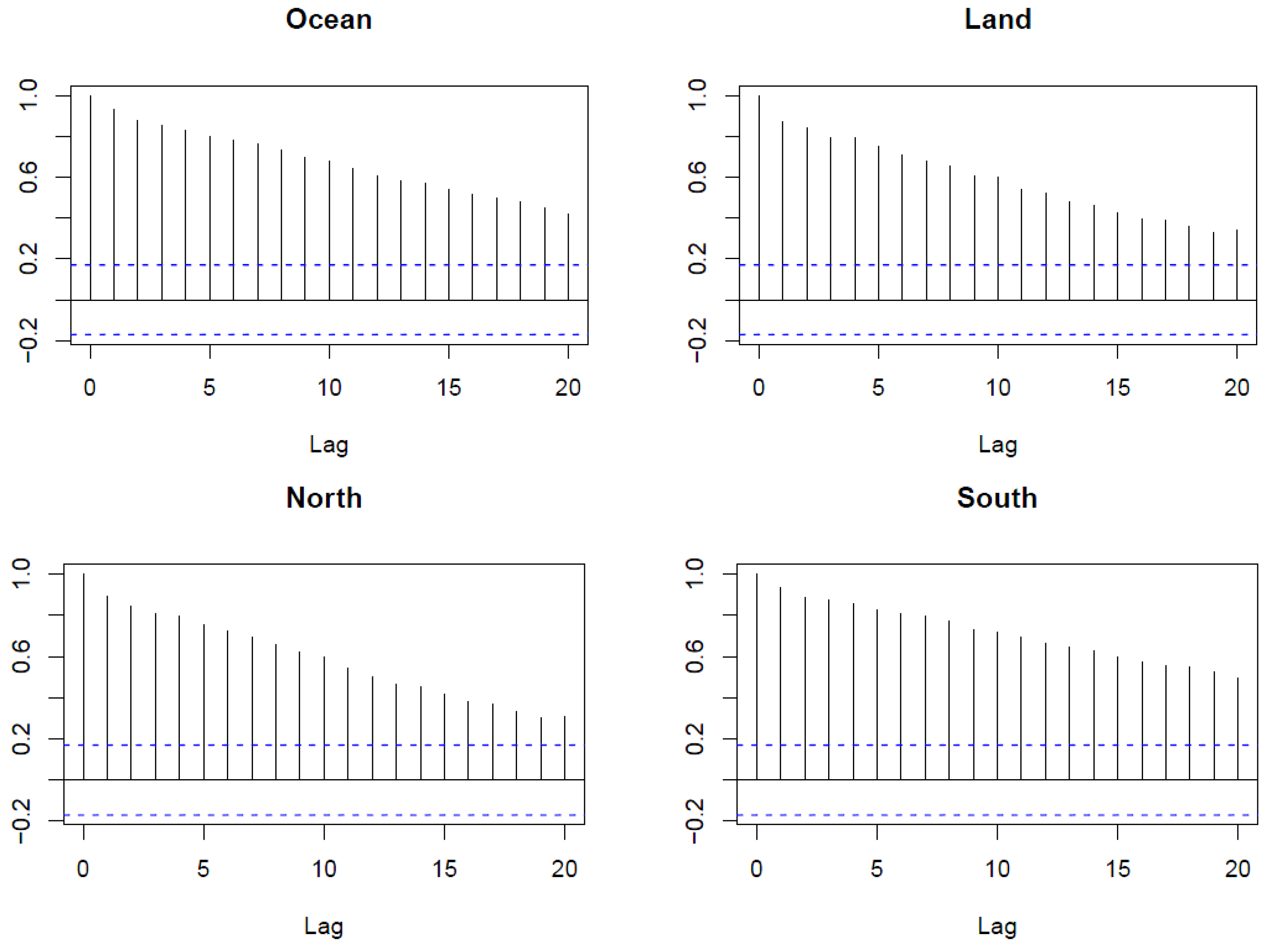
These global temperature anomaly data, with respect to the 20th century average, come from the Global Historical Climatology Network-Monthly (GHCN-M) data set and International Comprehensive Ocean-Atmosphere Data Set (ICOADS). The data span is from 1980 to 2012. These time series, shown in Figure 1, are available at [21]. Various subsets of this data set have been used in a number of studies (see, for example, [22,23]). The Auto Correlation Functions (ACFs) of the series and the Cross Correlation Functions (CCFs) are presented in Figure 2 and Figure 3, respectively. The ACF plots indicate that the series are nonstationary, since the ACFs decay very slowly.

We will build portfolios of ARMA models for these four series, and hence, by estimating the models for each portfolio, an estimate of the Hausdorff distance H among our time series will be obtained. Preliminarily, we have used the augmented Dickey Fuller (ADF) test in order to establish whether the considered series are stationary or non-stationary. We concluded that all four temperature time series are integrated of order one. These results are consistent with those obtained by Stern and Kaufmann ([24]), Liu and Rodriguez ([25]) and Mills ([26]). Now, in order to build a model portfolio for the considered time series, we identify ARMA models for the first differences of our time series. Bayesian Information Criterion (BIC) has been used to find the appropriate orders p and q of the AR and MA polynomials respectively.

The BIC values has been calculated for the ARMA($p,q$) models with $p,q\le 3$.

Table 1. Selection of the orders ($p,q$) of autoregressive moving average (ARIMA)($p,1,q$) models.

Series	O	L	N	S
Order	(2, 0)	(0, 1)	(0, 1)	(2, 0)

shows the orders ($p,q$) of ARMA models (for each time series) for which the value of the BIC, has been found to be minimum. The residual plots, reported in Figure 4, indicate no presence of serial correlation on the error term. The obtained portfolios of ARMA models for the four differenced series are:

• $P\left(O\right)=\left\{AR\left(2\right),MA\left(2\right)\right\}$,
• $P\left(S\right)=\left\{AR\left(2\right),MA\left(2\right),AR\left(3\right)\right\}$,
• $P\left(N\right)=\left\{MA\left(1\right),AR\left(3\right)\right\}$,
• $P\left(L\right)=\left\{MA\left(1\right)\right\}$.

By estimating the models for each portfolio, an estimate of the Hausdorff distance H is obtained.

Table 2. Estimates of the Hausdorff distance H.

Differenced Series	O	S	N	L
O	0.000	0.199	0.908	1.128
S	0.199	0.000	0.911	1.153
N	0.908	0.911	0.000	0.344
L	1.128	1.153	0.344	0.000

summarizes the results.

According to our notion of distance, the dynamic structure of the ocean temperature (O) and the dynamic structure of the southern temperature (S) seem to be very similar. On the contrary, both the series, O and S, seem to be very distant by the land temperature (L) and by the northern hemisphere temperature (N). Instead, a smaller distance separates the series L and N. The big thermal inertia of oceans, together with the uneven distribution of the land and sea (the Southern Hemisphere contains 80.9 percent water and 19.1 percent land, while the Northern Hemisphere is 60.7 percent water and 39.3 percent land) represents a possible explanation of our results. This conclusion is attractive since it links a statistical result to a physical mechanism.

5. Conclusions

This manuscript focuses on measuring the distance between two finite sets of invertible ARMA processes using the Hausdorff distance. In order to make this distance operative, a dissimilarity measure between two single ARMA processes (the AR metric) is considered. Of course other dissimilarity measures, e.g., the Mahalanobis distance between autoregressive models or the cepstral distance, could be used. We have chosen the AR metric since it is simple to compute and it is robust with respect to the presence of anomalous behavior in the data. Further, it is implemented for both stationary and non-stationary time series.

In order to show the usefulness of the proposed distance, two specific applications have been described. The first application consists of measuring the distance between two single ARMA series, let’s say x and y, by means of the Hausdorff distance between portfolios of ARMA models providing reasonably good fits of x and y. The second application uses the Hausdorff distance to compute distances between two VAR processes once these models are properly represented in terms of univariate ARMA processes. An empirical application is also presented.

References

- E.A. Maharaj. “Clusters of time series.” J. Classif. 17 (2000): 297–314. [Google Scholar] [CrossRef]
- T. Liao. “Clustering time series data—A survey.” Pattern Recognit. 38 (2005): 1857–1874. [Google Scholar] [CrossRef]
- R. Agrawal, C. Faloutsos, and A. Swami. “Efficient similarity search in sequence databases.” In Proceedings of the 4th International Conference on Data Organization and Algorithms FODO ’93, Chicago, IL, USA, 13–15 October 1993; New York, NY, USA: Springer Verlag, 1993. Number 730 in Lecture Notes in Computer Science. pp. 69–84. [Google Scholar]
- J. Caiado, N. Crato, and D. Peña. “A periodogram-based metric for time series classification.” Comput. Stat. Data Anal. 50 (2006): 2668–2684. [Google Scholar] [CrossRef] [Green Version]
- E. Otranto, and U. Triacca. “Measures to evaluate the discrepancy between direct and indirect model-based seasonal adjustment.” J. Off. Stat. 18 (2002): 551–530. [Google Scholar]
- F. Di Iorio, and U. Triacca. “Testing for Granger non-causality using the autoregressive metric.” Econ. Model. 33 (2013): 120–125. [Google Scholar] [CrossRef] [Green Version]
- L. Jin. “Comparing autocorrelation structures of multiple time series via the maximum distance between two groups of time series.” J. Stat. Comput. Simul. 85 (2015): 3535–3548. [Google Scholar] [CrossRef]
- P.J. Thomson, and P. de Souza. “Speech recognition using LPC distance measures.” In Handbook of Statistics 5 Time Series in the Time Domain. Edited by E.J. Hannan, P.R. Krishnaiah and M.M. Rao. Amsterdam, The Netherlands: North Holland, 1985, pp. 389–412. [Google Scholar]
- D. Piccolo. “A distance measure for classifying ARIMA models.” J. Time Ser. Anal. 11 (1990): 153–164. [Google Scholar] [CrossRef]
- M. Corduas, and D. Piccolo. “Time series clustering and classification by the autoregressive metric.” Comput. Stat. Data Anal. 52 (2008): 1860–1872. [Google Scholar] [CrossRef]
- E.A. Maharaj. “A significance test for classifying ARMA models.” J. Stat. Comput. Simul. 54 (1996): 305–331. [Google Scholar] [CrossRef]
- R.J. Martin. “A metric for ARMA processes.” IEEE Trans. Signal Proces. 48 (2000): 1164–1170. [Google Scholar] [CrossRef]
- P. Brockwell, and R. Davies. Time Series: Theory and Methods, 2nd ed. New York, NY, USA: Springer-Verlag, 1991. [Google Scholar]
- D.S. Poskitt, and A.R. Tremayne. “Determining a portfolio of linear time series models.” Biometrika 74 (1987): 125–137. [Google Scholar] [CrossRef]
- C. Chatfield. Time-Series Forecasting. London, UK: Chapman & Hall, 2000. [Google Scholar]
- G.E.P. Box, and G.M. Jenkins. Time Series Analysis: Forecasting and Control. San Francisco, CA, USA: Holden-Day, 1970. [Google Scholar]
- D. Faranda, B. Dubrulle, F. Daviaud, and F.M.E. Pons. “Probing turbulence intermittency via autoregressive moving-average models.” Phys. Rev. E 90 (2014): 061001. [Google Scholar] [CrossRef] [PubMed]
- D. Faranda, F.M.E. Pons, E. Giachino, S. Vaienti, and B. Dubrulle. “Early warnings indicators of financial crises via auto regressive moving average models.” Commun. Nonlinear Sci. Numer. Simul. 29 (2015): 233–239. [Google Scholar] [CrossRef]
- A. Sims. “Macroeconomics and reality.” Econometrica 48 (1980): 1–48. [Google Scholar] [CrossRef]
- A. Zellner, and F. Palm. “Time series analysis and simultaneous equation econometric models.” J. Econom. 2 (1974): 17–54. [Google Scholar] [CrossRef]
- “Climate at a Glance.” NOAA. Available online: http://www.ncdc.noaa.gov/cag/time-series/global (accessed on 10 June 2016).
- K.E. Trenberth. “Has there been a hiatus? ” Science 6249 (2015): 691–692. [Google Scholar] [CrossRef] [PubMed]
- U. Triacca, A. Pasini, and A. Attanasio. “Measuring persistence in time series of temperature anomalies.” Theor. Appl. Climatol. 118 (2014): 491–495. [Google Scholar] [CrossRef]
- D.I. Stern, and R.K. Kaufmann. “Econometric analysis of global climate change.” Environ. Model. Softw. 14 (1999): 597–605. [Google Scholar] [CrossRef]
- H. Liu, and G. Rodríguez. “Human activities and global warming: A cointegration analysis.” Environ. Model. Softw. 20 (2005): 761–773. [Google Scholar] [CrossRef] [Green Version]
- T.C. Mills. “Breaks and unit roots in global and hemispheric temperatures: An updated analysis.” Clim. Chang. 118 (2013): 745–755. [Google Scholar] [CrossRef]
© 2016 by the author; licensee MDPI, Basel, Switzerland. This article is an open access article distributed under the terms and conditions of the Creative Commons Attribution (CC-BY) license ( http://creativecommons.org/licenses/by/4.0/).