A Fast Algorithm for the Computation of HAC Covariance Matrix Estimators ^†

Abstract

This paper considers the algorithmic implementation of the heteroskedasticity and autocorrelation consistent (HAC) estimation problem for covariance matrices of parameter estimators. We introduce a new algorithm, mainly based on the fast Fourier transform, and show via computer simulation that our algorithm is up to 20 times faster than well-established alternative algorithms. The cumulative effect is substantial if the HAC estimation problem has to be solved repeatedly. Moreover, the bandwidth parameter has no impact on this performance. We provide a general description of the new algorithm as well as code for a reference implementation in R.

1. Introduction

This paper considers the heteroskedasticity and autocorrelation consistent (HAC) estimation of covariance matrices. This estimation problem arises in the construction of large-sample tests for the parameters in linear and nonlinear models. The HAC estimator for the covariance matrix of parameter estimators applies to a variety of model frameworks and estimation methods. Some examples are ordinary least squares (OLS), maximum likelihood, generalized method of moments (GMM) or instrumental variables (see Andrews [1], and Zeileis [2]). It also corresponds to the so-called sandwich estimator in the context of quasi-maximum likelihood (QML) estimation technique (cf. White [3], Chapter 8.3). In this connection we combine two essential topics to applied econometrics: robust covariance matrix estimation and fast computation of covariance matrix estimators.

In the last decades, several techniques for HAC covariance matrix estimation have been proposed in the literature, e.g., Andrews [1], Newey and West [4], White [5], MacKinnon and White [6]. These statistical methods go back to earlier literature, such as Jowett [7], Hannan [8], Brillinger [9]. Nowadays, these methods are widely used in econometric analysis. Beyond that, researchers require covariance matrices not only for the purpose of some hypothesis tests, but also as stand-alone functions which can be used in various statistical methods. This is becoming more and more relevant as pointed out in Cribari-Neto and Zarkos [10]. In spite of the vast econometric literature on this subject, little econometric software is available for the computation of HAC covariance matrix estimators.

The aim of this paper is to show that the computing time for HAC covariance matrix estimators can be decreased massively by using given information about the structure of the HAC covariance matrix estimators together with some matrix algebra. Particularly, we exploit the evaluation of a circulant matrix product, which can be efficiently calculated using the fast Fourier transform. The same calculation idea is employed by Wood and Chan [11] for the simulation of stationary Gaussian processes with prescribed covariance matrix as well as by Jensen and Nielsen [12] for the calculation of fractional differences.

We compare our new algorithm with two popular statistic algorithms: the algorithm by Roncalli [13], which is written for the statistical software GAUSS (cf. Aptech Systems [14]) and the algorithm by Zeileis [15] written for R (cf. R Development Core Team [16]), as well as with the lesser-known algorithm by Kyriakoulis [17] for MATLAB (cf. MathWorks [18]). According to our results, our new algorithm is up to ~20 times faster than the algorithms by Roncalli and Zeileis. The saved time can increase up to a few minutes for only one HAC estimation depending on the settings of the estimation problem. This is particularly relevant for the QML estimation of generalized autoregressive conditional heteroskedastic (GARCH) models (cf. Zivot [19]) and the estimation of stochastic volatility (SV) models via QML (cf. Ruiz [20]) or GMM (cf. Renault [21]) based on large financial datasets with high frequency sampling or multivariate structure. Another application area is the GMM estimation of multifractal volatility models (cf. Bacry et al. [22], Lux [23]), which proves to be a time consuming issue even in the univariate case with daily data. Thus reliable estimation results for the Multifractal Random Walk model require a data sample of size N > 2000, all the more the asymptotic normality of the GMM estimates can be reached only for sample sizes not less than ca. 16,000 data points (cf. Bacry et al. [24]). The cumulative effect is substantial if the HAC estimation problem has to be solved repeatedly (e.g., in the case of an iterated GMM estimation or for the purpose of simulation and forecast studies.).

Moreover, our algorithm does not employ the bandwidth parameter explicitly. Its performance is independent of the value of the bandwidth parameter as contrasted with the algorithms by Roncalli and Zeileis.

The paper is organized as follows. In Section 2 we give an overview on the HAC estimation problem and some of its application fields and introduce the notation we use. Section 3 combines some matrix algebra results and the structure of HAC estimators in order to introduce the new algorithm. In Section 4 we discuss the alternative algorithms. Section 5 investigates the performance issues of our new algorithm as compared with the alternative algorithms. We replicate the HAC computation steps in Chaussé and Xu [25] for the estimation of a SV model with high frequency data as well as in Lux et al. [26] for the purpose of a forecast study and report the computing time. We show that the new algorithm outperforms the other algorithms in the majority of cases we analyse. There are some isolated cases where our algorithm performs more slowly. However the computational cost is below 1 millisecond, which should be irrelevant in practice. The R-Codes for the different HAC covariance matrix estimators are given in the Appendix.

2. HAC Covariance Matrix Estimation

2.1. The Estimation Problem

We consider ${\left(a_t\right)}_{t\in \mathbb{Z}}$ a stationary ergodic q-dimensional stochastic process of mean zero and ${\left({\mathsf{\Gamma }}_{\tau }\right)}_{\tau \in \mathbb{Z}}$ its autocovariance matrices

$${\mathsf{\Gamma }}_{\tau }=\mathrm{E}\left[a_t{a}_{t+\tau }^{\prime }\right].$$

(1)

We want to estimate the quantity

$$S_N=\frac{1}{N}\sum _{s=1}^N\sum _{t=1}^N\mathrm{E}\left[a_t{a}_s^{\prime }\right],$$

(2)

where N denotes the number of given observations. $S_N$ can be also written as (cf. Smith [27])

$$S_N={\mathsf{\Gamma }}_0+\sum _{\tau =1}^{N-1}\frac{N-\tau }{N}\left({\mathsf{\Gamma }}_{\tau }+{\mathsf{\Gamma }}_{-\tau }\right).$$

(3)

This estimation problem can be solved in the limit for $N\to \infty$, i.e.,

$$S=\underset{N\to \infty }{lim}{S}_N=\sum _{\tau =-\infty }^{\infty }{\mathsf{\Gamma }}_{\tau }=f\left(0\right)$$

(4)

with $f\left(0\right)$ the spectral density matrix of the process $\left(a_t\right)$ in 0. The estimation of S is a nonparametric spectral estimation problem with the corresponding lag window spectral estimator

$${\widehat{S}}_N={\widehat{\mathsf{\Gamma }}}_0+\sum _{\tau =1}^{N-1}{\omega }_{\tau ,N}\left({\widehat{\mathsf{\Gamma }}}_{\tau }+{\widehat{\mathsf{\Gamma }}}_{\tau }^{\prime }\right).$$

(5)

${\widehat{\mathsf{\Gamma }}}_{\tau }$ denotes the empirical autocovariance matrix of lag τ

$${\widehat{\mathsf{\Gamma }}}_{\tau }=\frac{1}{N}\sum _{t=1}^{N-\tau }{a}_t{a}_{t+\tau }^{\prime }$$

(6)

with $0\le \tau \le N-1$ and ${\omega }_{\tau ,N}$ is a function of weights (cf. Newey and West [4]). ${\widehat{S}}_N$ is weakly consistent for given choice of ${\omega }_{\tau ,N}$ and it is called a Heteroskedasticity and Autocorrelation Consistent (HAC) covariance matrix estimator for reasons to be explained below.

Let the bandwidth parameter $b_N$ control the number of nonzero weights, ${\omega }_{\tau ,N}=0$ for $\tau >b_N$. Then we can also write Equation (5) as follows

$${\widehat{S}}_N={\widehat{\mathsf{\Gamma }}}_0+\sum _{\tau =1}^{b_N}{\omega }_{\tau ,N}\left({\widehat{\mathsf{\Gamma }}}_{\tau }+{\widehat{\mathsf{\Gamma }}}_{\tau }^{\prime }\right).$$

(7)

Note that the algorithm considered in this paper does not require the specification of a bandwidth parameter. In the following we suppress the index N for reasons of simplicity and write ${\omega }_{\tau }$ and b, respectively.

2.2. Application

This estimation problem can be applied to various econometric fields depending on the choice of $\left(a_t\right)$. Its main interest resides in the construction of large-sample tests. Many parameter estimators ${\widehat{\theta }}_N$ in nonlinear dynamic models satisfy

$$\sqrt{N}\left({\widehat{\theta }}_N-{\theta }_0\right)\stackrel{d}{\to }\mathcal{N}\left(0,MS{M}^{\prime }\right)$$

(8)

with ${\theta }_0$ the true parameter value to be estimated, M a non-random matrix and S given in (4). See Andrews [1] on the estimation of M. One can construct tests about the value of ${\theta }_0$ based on the approximate distribution of ${\widehat{\theta }}_N$ in large samples

$${\widehat{\theta }}_N\stackrel{·}{\sim }\mathcal{N}\left({\theta }_0,\frac{1}{N}MS{M}^{\prime }\right)$$

(9)

where S can be estimated by ${\widehat{S}}_N$ in (5). It is now obvious why we call ${\widehat{S}}_N$ a covariance matrix estimator.

2.3. The Case of the OLS Estimator

Consider the linear model $Y=X\theta +u$ with the OLS estimator $\widehat{\theta }={\left(X^{\prime }X\right)}^{-1}{X}^{\prime }Y$ and

$$\begin{array}{cc}\hfill \mathrm{Cov}\left[\widehat{\theta }\right]& ={\left(X^{\prime }X\right)}^{-1}{X}^{\prime }\mathrm{Cov}\left[Y\right]X{\left(X^{\prime }X\right)}^{-1}\hfill \end{array}$$

(10)

$$\begin{array}{cc}& ={\left(X^{\prime }X\right)}^{-1}{X}^{\prime }\mathrm{E}\left[u{u}^{\prime }\right]X{\left(X^{\prime }X\right)}^{-1}.\hfill \end{array}$$

(11)

In the case of homoskedastic and uncorrelated errors, $\mathrm{E}\left[u{u}^{\prime }\right]={\sigma }^{2}I$, the covariance matrix of $\widehat{\theta }$ simplifies to

$$\mathrm{Cov}\left[\widehat{\theta }\right]={\sigma }^2{\left(X^{\prime }X\right)}^{-1}$$

(12)

and it can be easily estimated by

$$\widehat{\mathrm{Cov}}\left[\widehat{\theta }\right]=s^2{\left(X^{\prime }X\right)}^{-1}$$

(13)

with $s^2$ an unbiased estimator for ${\sigma }^2$. In the general case of heteroskedasticity and dependence of unknown forms of the error term u one can estimate the following asymptotic covariance matrix

$$\begin{array}{cc}\hfill \underset{N\to \infty }{lim}\mathrm{Cov}\left[\sqrt{N}\left({\widehat{\theta }}_N-{\theta }_0\right)\right]& =\underset{N\to \infty }{lim}N{\left(X^{\prime }X\right)}^{-1}{X}^{\prime }\mathrm{E}\left[u{u}^{\prime }\right]X{\left(X^{\prime }X\right)}^{-1}\hfill \end{array}$$

(14)

$$\begin{array}{cc}& =\underset{N\to \infty }{lim}{\left(\frac{1}{N}{X}^{\prime }X\right)}^{-1}{S}_N{\left(\frac{1}{N}{X}^{\prime }X\right)}^{-1}\hfill \end{array}$$

(15)

$$\begin{array}{cc}& =\underset{N\to \infty }{lim}{\left(\frac{1}{N}{X}^{\prime }X\right)}^{-1}S\underset{N\to \infty }{lim}{\left(\frac{1}{N}{X}^{\prime }X\right)}^{-1}\hfill \end{array}$$

(16)

with

$$S=\underset{N\to \infty }{lim}{S}_N=\underset{N\to \infty }{lim}\frac{1}{N}{X}^{\prime }\mathrm{E}\left[u{u}^{\prime }\right]X=\underset{N\to \infty }{lim}\frac{1}{N}\sum _{t=1}^N\sum _{s=1}^N\mathrm{E}\left[X_t^{\prime }{u}_t{\left(X_s^{\prime }{u}_s\right)}^{\prime }\right].$$

(17)

This estimation can be performed using the HAC covariance matrix estimator (cf. formula (5)) based on the process $\left(a_t\right)=\left(X_t^{\prime }{u}_t\right)$.

The OLS estimator satisfies

$$\sqrt{N}\left({\widehat{\theta }}_N-{\theta }_0\right)\stackrel{d}{\to }\mathcal{N}\left(0,Q^{-1}S{Q}^{-1}\right)$$

(18)

with $Q={lim}_{N\to \infty }\frac{1}{N}{X}^{\prime }X$ a finite nonsingular matrix and respectively in large samples

$${\widehat{\theta }}_N\stackrel{·}{\sim }\mathcal{N}\left({\theta }_0,\frac{1}{N}{Q}^{-1}S{Q}^{-1}\right).$$

(19)

2.4. The Case of the GMM Estimator

Consider the model-free GMM estimation of ${\theta }_0$ using q moment conditions. In this case, the process $\left(a_t\right)$ contains the q-dimensional deviation of the empirical moments $m_t={\left(m_{i,t}\right)}_{1\le i\le q}$ from their theoretical counterparts $M_t\left(\theta \right)={\left(M_{i,t}\right)}_{1\le i\le q}$ with

$$a_t\left(\theta \right)=M_t\left(\theta \right)-m_t.$$

(20)

The GMM estimator is given by

$$\widehat{\theta }=\underset{\theta \in \mathsf{\Theta }}{argmin}\left(\frac{1}{N}\sum _t{a}_t^{\prime }\left(\theta \right)\right)W\left(\frac{1}{N}\sum _t{a}_t\left(\theta \right)\right)$$

(21)

with W some weighting matrix (Hall [28]). Under some regularity conditions the GMM estimator is weakly consistent and asymptotically normally distributed

$$\sqrt{N}\left({\widehat{\theta }}_N-{\theta }_0\right)\stackrel{d}{\to }\mathcal{N}(0,MS{M}^{\prime }),$$

(22)

where M is a non-random matrix and

$$\begin{array}{cc}\hfill S& =\underset{N\to \infty }{lim}N·\mathrm{Cov}\left[\frac{1}{N}\sum _{q=1}^N{a}_t\right]\hfill \end{array}$$

(23)

$$\begin{array}{cc}& =\underset{N\to \infty }{lim}N·\mathrm{E}\left[\frac{1}{N^2}\sum _{t=1}^N{a}_t\sum _{s=1}^N{a}_s^{\prime }\right]\hfill \end{array}$$

(24)

$$\begin{array}{cc}& =\underset{N\to \infty }{lim}\frac{1}{N}\sum _{t=1}^N\sum _{s=1}^N\mathrm{E}\left[a_t{a}_s^{\prime }\right].\hfill \end{array}$$

(25)

Again we employ the HAC covariance matrix estimator (cf. formula (5)) in order to estimate S.

3. The Algorithm

In this paper, we introduce a fast algorithm for the computation of the HAC covariance matrix estimator ${\widehat{S}}_N$ in (5). This is based on the equivalent representation (cf. Kyriakoulis [17])

$${\widehat{S}}_N=\frac{1}{N}{A}^{\prime }T\left(\omega \right)A$$

(26)

with $A\in {\mathbb{R}}^{N\times q}$ and

$$A=\left(\begin{array}{c}{a}_1^{\prime }\\ a_2^{\prime }\\ ⋮\\ a_N^{\prime }\end{array}\right).$$

(27)

The matrix $T\left(\omega \right)$ denotes the symmetric $N\times N$ Toeplitz matrix with first column ω given by the weights

$$\omega ={\left(\begin{array}{ccccc}1& {\omega }_1& {\omega }_2& \dots & {\omega }_{N-1}\end{array}\right)}^{\prime }.$$

(28)

For a more memory space-efficient computation of the matrix product $T\left(\omega \right)A$ we are using a special circulant matrix (cf. Van Loan [29]). Therefore, we embed the Toeplitz matrix $T\left(\omega \right)$ in a symmetric circulant matrix $C\left({\omega }^{*}\right)\in {\mathbb{R}}^{2N\times 2N}$ with

$${\omega }^{*}={\left(\begin{array}{cccccccccc}1& {\omega }_1& {\omega }_2& \dots & {\omega }_{N-1}& 0& {\omega }_{N-1}& {\omega }_{N-2}& \dots & {\omega }_1\end{array}\right)}^{\prime }.$$

(29)

Furthermore, we construct the $2N\times q$ matrix $A^{*}$

$$A^{*}=\left(\begin{array}{c}A\\ 0_{N\times q}\end{array}\right)$$

(30)

by adding a $N\times q$ matrix containing only zeros at the bottom of A.

Remark 1.

• The Toeplitz matrix $T\left(\omega \right)$ is given by the first N rows and first N columns of $C\left({\omega }^{*}\right)$, i.e.,

  $$T\left(\omega \right)=C_{1:N,1:N}\left({\omega }^{*}\right).$$

  (31)

  Generally we denote with $M_{a:b,c:d}\in {\mathbb{R}}^{m\times n}$ a sub-matrix of M containing the rows from a to b and the columns from c to d ($a,b,c,d\in \mathbb{N}$, $1\le a\le b\le m$ and $1\le c\le d\le n$).
• The necessary product $T\left(\omega \right)A$ is given by

  $$C_{1:N,•}\left({\omega }^{*}\right)A^{*}=C_{1:N,1:N}\left({\omega }^{*}\right)A=T\left(\omega \right)A.$$

  (32)

  Thus, the fast evaluation of $C\left({\omega }^{*}\right)A^{*}$ permits fast evaluation of $T\left(\omega \right)A$.

The following theorem explains how the matrix product $T\left(\omega \right)A$ (cf. formula (26)) can be computed in a fast way by means of the discrete Fourier transform (DFT) and its inverse transform. It provides the basis for our new algorithm.

Theorem 1 (Circulant matrix and its eigenvalues and eigenvectors).

Let $C\left(c\right)\in {\mathbb{R}}^{n\times n}$ be a circulant matrix with first column $c={\left(\begin{array}{ccc}{c}_1& \dots & c_n\end{array}\right)}^{\prime }$ and let $V\mathsf{\Lambda }{V}^{*}$ be the matrix decomposition of $C\left(c\right)$, i.e.,

$$C\left(c\right)=V\mathsf{\Lambda }{V}^{*}.$$

(33)

Thereby, ${\lambda }_k$ ($k=1,\dots ,n$) are the eigenvalues of $C\left(c\right)$ and $v_k$ ($k=1,\dots ,n$) the corresponding eigenvectors. The matrix Λ is diagonal with $\mathsf{\Lambda }=diag({\lambda }_1,\dots ,{\lambda }_n)$ and V is a matrix containing the eigenvectors, i.e., $V=\left(\begin{array}{ccc}{v}_1& \dots & v_n\end{array}\right)$. The matrix $V^{*}$ is the complex conjugate of V. Then, the following properties hold true:

1.

The eigenvalues ${\lambda }_k$ are the discrete Fourier transform (DFT) of the column vector c, i.e.,

$${\lambda }_k=\sum _{j=1}^{n}exp\left(-\frac{2(j-1)k\pi i}{n}\right)c_j$$

(34)

for $k=1,\dots ,n$.

2.

The orthornomal left eigenvectors $v_k$ ($k=1,\dots ,n$) are given by

$$v_k=n^{-\frac{1}{2}}\left(\begin{array}{ccccc}1& r_k& r_k^2& \dots & r_k^{n-1}\end{array}\right)$$

(35)

with $r_k=exp\left(\frac{2(k-1)\pi i}{n}\right)$.

3.

The product $V^{*}x$, for any $x\in {\mathbb{R}}^n$, is given by the DFT of x.

4.

The product $y=Vx\in {\mathbb{R}}^n$, for any $x\in {\mathbb{R}}^n$, is given by the inverse discrete Fourier Transform (IDFT) of x, i.e.,

$$y_k=\frac{1}{n}\sum _{j=1}^{n}exp\left(-\frac{2(j-1)k\pi i}{n}\right)x_j$$

(36)

for $k=1,\dots ,n$.

Proof. 

See Brockwell and Davis [30], Gray [31] or Golub and Van Loan [32]. ☐

We now introduce the new algorithm (cf. Algorithm 1) for the computation of HAC covariance matrix estimators on the basis of Theorem 1. In the following we assume that the weights ${\omega }_{\tau }$ ($\tau =1,\dots ,N-1$) are known.

Algorithm 1.

The algorithm is given in five steps while step three is subdivided into three steps.

1.

Compute the eigenvalues ${\lambda }_i$ ($i=1,\dots ,2N$) of $C\left({\omega }^{*}\right)$ using Equation (34) with

$${\omega }^{*}={\left(\begin{array}{cccccccccc}1& {\omega }_1& {\omega }_2& \dots & {\omega }_{N-1}& 0& {\omega }_{N-1}& {\omega }_{N-2}& \dots & {\omega }_1\end{array}\right)}^{\prime }.$$

(37)

2.

Construct the matrix $A^{*}$ with dimension $2N\times q$ from

$$A^{*}=\left(\begin{array}{c}A\\ 0_{N\times q}\end{array}\right)$$

(38)

using A from Equation (27).

3.

For all $j\in \{1,\dots ,q\}$ compute the columns of the matrix $C\left({\omega }^{*}\right)A^{*}$. These columns are written as $C\left({\omega }^{*}\right)A_j^{*}=V\mathsf{\Lambda }{V}^{*}{A}_j^{*}$ while $A_j^{*}$ is the j-th column of $A^{*}$. This computation is done in three steps:

(a) 

Determine $V^{*}{A}_j^{*}$ given by the DFT of $A_j^{*}$.

(b) 

Multiply for all $i\in \{1,\dots ,2N\}$ the i-th entry of the vector $V^{*}{A}_j^{*}$ with the eigenvalue ${\lambda }_i$, in order to construct $\mathsf{\Lambda }{V}^{*}{A}_j^{*}$.

(c) 

Determine $C\left({\omega }^{*}\right)A_j^{*}=V\mathsf{\Lambda }{V}^{*}{A}_j^{*}$ given by the IDFT of $\mathsf{\Lambda }{V}^{*}{A}_j^{*}$.

4.

Select the upper $N\times q$ block of $C\left({\omega }^{*}\right)A^{*}$. This upper block results in $T\left(\omega \right)A$, i.e.,:

$${\left(C\left({\omega }^{*}\right)A^{*}\right)}_{1:N,•}=T\left(\omega \right)A$$

(39)

5.

Determine ${\widehat{S}}_N=\frac{1}{N}{A}^{\prime }T\left(\omega \right)A$.

4. Alternative Algorithms

In this paper, we compare our new algorithm with three alternative algorithms currently used. The first algorithm that we consider was developed by Roncalli [13] and can be found in the time series library TSM (Time Series and Wavelets for Finance) for the statistical software GAUSS (cf. Aptech Systems [14]). Here the computation of HAC estimators ${\widehat{S}}_N$ is implemented by means of a for-loop according to expression (7) combined with an ingenious matrix product, which enables the fast computation of the autocovariance matrices ${\widehat{\mathsf{\Gamma }}}_{\tau }$:

$${\widehat{\mathsf{\Gamma }}}_{\tau }=\frac{1}{N}{A}^{\prime }\left(\begin{array}{c}{0}_{\tau \times q}\\ A(1:(N-\tau \left)\right)\end{array}\right)$$

(40)

Algorithm 2 (Roncalli).

1.

Determine ${\widehat{\mathsf{\Gamma }}}_0=\frac{1}{N}{A}^{\prime }A$ and set $L={\widehat{\mathsf{\Gamma }}}_0$.

2.

For τ from 1 to b determine ${\widehat{\mathsf{\Gamma }}}_{\tau }$ according to (40) and update $L=L+{\omega }_{\tau }\left({\widehat{\mathsf{\Gamma }}}_{\tau }+{\widehat{\mathsf{\Gamma }}}_{\tau }^{\prime }\right)$.

3.

Determine ${\widehat{S}}_N=L$.

The second algorithm by Zeileis [15] is part of the “sandwich” package for the statistical software R (cf. R Development Core Team [16]). This algorithm is similar to Roncalli’s algorithm except for the calculation procedure for ${\widehat{\mathsf{\Gamma }}}_{\tau }$ in Step 2. His procedure is less efficient than Roncalli’s as it requires the sequential updating of two matrices instead of one.

Algorithm 3 (Zeileis).

1.

Determine ${\widehat{\mathsf{\Gamma }}}_0=\frac{1}{N}{A}^{\prime }A$ and set $L={\widehat{\mathsf{\Gamma }}}_0$.

2.

For τ from 1 to b determine ${\widehat{\mathsf{\Gamma }}}_{\tau }=\frac{1}{N}{\left(A((\tau +1):N)\right)}^{\prime }A(1:(N-\tau ))$ and update $L=L+{\omega }_{\tau }\left({\widehat{\mathsf{\Gamma }}}_{\tau }+{\widehat{\mathsf{\Gamma }}}_{\tau }^{\prime }\right)$.

3.

Determine ${\widehat{S}}_N=L$.

Finally, the algorithm by Kyriakoulis [17] for MATLAB (cf. MathWorks [18]) excels in terms of its elegance and simplicity. This algorithm avoids the resource-intensive recursive summations employed above using instead expression (26) and is the basis for the new algorithm introduced in the previous section. It consists of only two steps:

Algorithm 4 (Kyriakoulis).

1.

Construct the symmetric Toeplitz matrix $T\left(\omega \right)$ with the first column

$$\omega ={\left(\begin{array}{ccccc}1& {\omega }_1& {\omega }_2& \dots & {\omega }_{N-1}\end{array}\right)}^{\prime }.$$

(41)

2.

Determine ${\widehat{S}}_N=\frac{1}{N}{A}^{\prime }T\left(\omega \right)A$.

A big drawback of this algorithm is the memory space-inefficient handling of the $N\times N$ matrix $T\left(\omega \right)$. On account of this the program runs out of memory and fails to compute ${\widehat{S}}_N$ for series longer than $N=\mathrm{10,000}$ data points. This problem could be solved within the scope of our algorithm, which does not employ the matrix $T\left(\omega \right)$ explicitly.

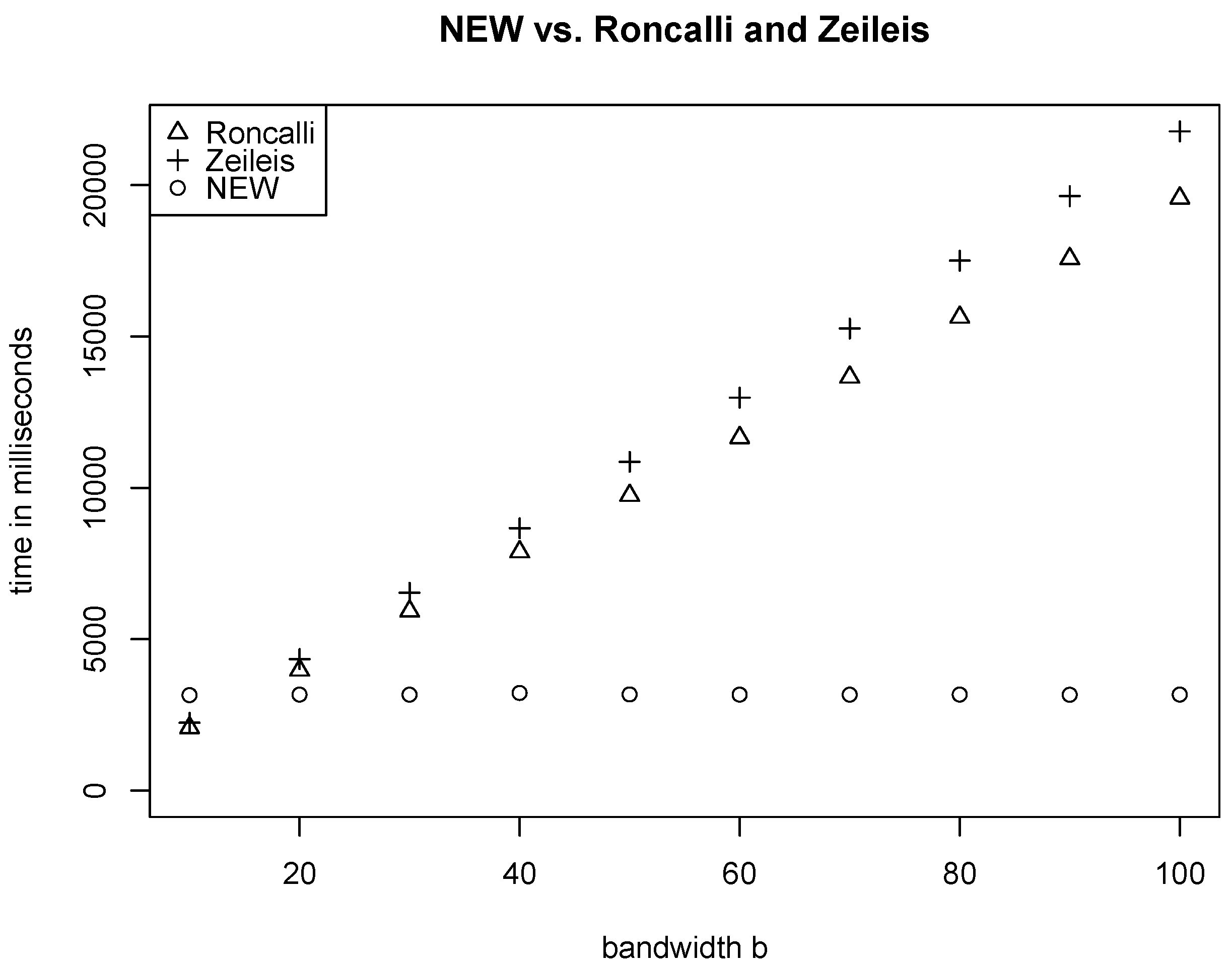
5. Comparing Different Algorithms for the Computation of HAC Covariance Matrix Estimators

In this section we present the gains in absolute and relative computing times that are achieved by our new algorithm compared with the three alternative algorithms discussed in the previous section.

All four algorithms were programmed and run in R (cf. R Development Core Team [16]) for reasons of comparability.

Remark 2.

• We used the “fftwtools”-package of R for the fft-function. The four algorithms run a little bit faster when using the “compiler”-package of R , but relative computing times are nearly the same.
• There is a little difference in the results between the algorithms {Roncalli [13], Zeileis [15]} and {NEW, Kyriakoulis [17]}. The difference is somewhere near machine precision ($\sim exp\left(-16\right)$) and the practical relevance should be very little.

We used the following hard- and software:

• Intel i5 2.90 GHz
• 8GB RAM
• R 3.3.2
• Windows 10 Professional 64bit

We measured the computing time for different values of b, N and q. The matrix A was randomly generated for every set of $(b,N,q)$, using a normally distributed random number generator with mean 0 and standard deviation 10. Nonetheless neither the distribution nor the parameters of the random number generator influenced the results significantly. All four algorithms were applied to the same matrix A (given b, N and q). After each application all variables in R except for A, b, N and q were deleted.

We used the weights ${\omega }_{\tau }$ for the quadratic spectral kernel function, since this kernel function is probably most frequently used in the literature (cf. Zeileis [15]). An overview of different weights can be found in Andrews [1]. The results of the computing times are given in

Table 1. Absolute computing time (in milliseconds) for different values of b, N and q (Note: R runs out of memory in the “blank”-cases.).

		New Algorithm			Roncalli			Zeileis			Kyriakoulis
	N	q			q			q			q
		10	20	30	10	20	30	10	20	30	10	20	30
$b=30$	5000	11	24	31	21	76	156	24	89	165	1404	1603	1806
	10,000	25	54	74	49	166	334	54	173	340	5654	6827	7398
	50,000	125	319	447	267	905	1738	291	947	1797
	100,000	287	642	892	571	1893	3521	635	2066	3685
	200,000	628	1195	1768	1185	3855	7313	1280	4321	7538
	500,000	1523	3006	4485	2963	9628	18,145	3260	9849	18,929
	1,000,000	3201	6727	9809	5862	18,497	36,687	6545	19,627	37,678
$b=60$	5000	9	22	31	46	149	320	56	160	342	1388	1606	1807
	10,000	27	49	75	95	324	646	108	344	672	6067	6526	7375
	50,000	121	319	446	547	1850	3530	595	1950	3704
	100,000	330	579	851	1108	3746	6971	1238	4016	7242
	200,000	626	1254	1823	2326	7765	14,474	2550	8255	14,974
	500,000	1502	2977	4682	6081	19,021	36,469	6427	19,807	37,544
	1,000,000	3150	6398	9833	11,565	36,816	72,326	12,972	39,166	74,822
$b=100$	5000	10	25	34	78	248	512	88	266	539	1382	1609	1907
	10,000	27	52	76	156	546	1065	178	589	1148	5770	6832	7699
	50,000	121	319	454	950	2990	5917	1025	3336	6380
	100,000	331	580	927	1832	6204	11,650	2063	6532	12,068
	200,000	630	1250	1749	3884	12,687	24,201	4172	13,598	25,489
	500,000	1511	2991	4872	9763	31,210	60,453	10,753	33,047	62,455
	1,000,000	3177	6441	9855	19,424	62,593	121,815	21,667	65,241	125,517

in absolute time (in milliseconds) and in

Table 2. Relative computing times (compared to our new algorithm) for different values of b, N and q (Note: R runs out of memory in the “blank”-cases.).

		Roncalli			Zeileis			Kyriakoulis
	N	q			q			q
		10	20	30	10	20	30	10	20	30
$b=30$	5000	1.99	3.09	5.09	2.24	3.65	5.38	45.73	74.84	23.89
	10,000	1.94	3.08	4.50	2.17	3.22	4.58	76.24	140.40	44.61
	50,000	2.14	2.83	3.89	2.33	2.96	4.02
	100,000	1.99	2.95	3.95	2.21	3.22	4.13
	200,000	1.89	3.23	4.14	2.04	3.61	4.26
	500,000	1.95	3.20	4.05	2.14	3.28	4.22
	1,000,000	1.83	2.75	3.74	2.04	2.92	3.84
$b=60$	5000	4.92	6.90	10.35	6.00	7.39	11.06	44.84	35.22	12.10
	10,000	3.51	6.67	8.59	4.01	7.06	8.93	80.65	68.75	22.75
	50,000	4.54	5.80	7.92	4.94	6.11	8.31
	100,000	3.35	6.47	8.19	3.75	6.93	8.51
	200,000	3.72	6.19	7.94	4.08	6.58	8.21
	500,000	4.05	6.39	7.79	4.28	6.65	8.02
	1,000,000	3.67	5.75	7.36	4.12	6.12	7.61
$b=100$	5000	7.85	9.84	15.03	8.78	10.54	15.82	40.56	20.50	7.68
	10,000	5.70	10.58	14.08	6.48	11.42	15.17	76.24	43.68	14.11
	50,000	7.88	9.37	13.02	8.50	10.45	14.04
	100,000	5.54	10.70	12.57	6.24	11.27	13.02
	200,000	6.17	10.15	13.83	6.62	10.88	14.57
	500,000	6.46	10.44	12.41	7.11	11.05	12.82
	1,000,000	6.11	9.72	12.36	6.82	10.13	12.74

in relative time (compared with our new algorithm).

Obviously, in Table 1 one can see that our new algorithm has the advantage that the bandwidth b has no impact on its performance, while it has for the Roncalli and Zeileis algorithms. The saved time can increase up to a few minutes for only one HAC estimation depending on the settings of the estimation problem.

Figure 1 shows a plot of absolute computation times of our new algorithm against the algorithms of Roncalli [13] and Zeileis [15] for different bandwidths b ($N={10}^6$ and $q=10$). One can see again that our new algorithm is independent of the bandwidth b while the algorithms of Roncalli [13] and Zeileis [15] are not. This encouraging performance opens up new possibilities of using large bandwidths in combination with large datasets. We leave this issue for future exploration.

Let us exemplify how Table 2 needs to be read. For example consider the case $b=60$, $N={10}^5$ and $q=30$. Then the algorithm proposed by Roncalli [13] needs 8.19 times more computation time compared with our new algorithm and the algorithm proposed by Zeileis [15] needs 8.51 times more computation time compared with our new algorithm.

Table 2 can be summarized as follows:

• Compared with the algorithm proposed by Roncalli [13] our new algorithm is between 1.83 times and 15.03 times faster.
• Compared with the algorithm proposed by Zeileis [15] our new algorithm is between 2.04 and 15.82 times faster.
• Compared with the algorithm proposed by Kyriakoulis [17] our new algorithm is between 7.68 and 140.40 times faster, while the algorithm proposed by Kyriakoulis [17] runs out of memory for $N>{10}^4$.

Overall, our new algorithm is faster than any of the compared algorithms. The time saved while using the new algorithm can increase considerably, especially if the HAC estimation problem has to be solved repeatedly. For example, the iterated GMM estimation procedure requires an update of the estimated covariance matrix in each step. If we consider 50 estimation steps, then our new algorithm can save up to ~95 min compared with the algorithms proposed by Roncalli [13] or Zeileis [15] ($b=100$, $N={10}^6$ and $q=30$). Even in the case of a shorter dataset ($N={10}^5$) we would still save up to ~9 minutes as compared with the alternative algorithms ($b=100$, $N={10}^5$ and $q=30$).

Figure 2 shows different relative computing times as a function of the sample size ($N\in \{{10}^2,5·{10}^2,{10}^3,5·{10}^3,{10}^4,5·{10}^4,{10}^5,2·{10}^5,5·{10}^5,{10}^6\}$). One can see that our new algorithm outperforms in the majority of parameter constellations. Only in the case of a small N ($N\in \{100,500\}$) combined with a small bandwidth ($b=30$) and only few moment conditions ($q=10$) does our algorithm perform more slowly. This is in accordance with the performance pattern in Jensen and Nielsen [12]. However, the computational cost is below 1 millisecond, which should be irrelevant in practice. Our algorithm reaches its highest performance approximately for N between 500 and 1000. After $N=1000$ the performance of our new algorithm reduces, but still remains better than Roncalli [13] or Zeileis [15]. At the same time, the absolute computing times increase significantly, which leads to a considerable difference in computational speed between the competing algorithms. This is also illustrated below.

We replicate the HAC estimation problem in two empirical applications and report the computing time for the three competing algorithms.

Remark 3.

We used the “fftwtools”-package of R for the fft-function. Additionally, the time series was padded with zeros such that the total length of the series was a power of two.

The first empirical application is the estimation of a generalized asymmetric SV model with realized volatility (GASV-RV) in Chaussé and Xu [25] based on high frequency financial data. The estimation sample spans 5 years (2003–2008) and a total of $N=\mathrm{1,456,650}$ observations. The authors consider four different GMM estimation procedures, each of them using the HAC covariance matrix estimation and various sets of moment conditions with $q=36$ moments at most. We replicated this estimation problem and estimated only the corresponding HAC covariance matrices based on randomly generated data, so that our new algorithm can directly be compared with the other ones. According to our results in

Table 3. Computation times and gain in time in minutes for our new algorithm compared to the ones proposed by Roncalli [13] and Zeileis [15] for the empirical applications in Chaussé and Xu [25] and Lux et al. [26].

	Time in Minutes
	Chaussé and Xu		Hansen et al.		Lux et al.
	one est.	full est.	one est.	full est.	“turbulent”	“full”
Roncalli	1.38	33.03	1.67	193.40	17.31	35.80
Zeileis	1.47	35.23	1.68	195.20	19.71	40.41
NEW	0.39	9.32	0.66	76.42	10.55	22.84
gain in time NEW vs. Roncalli	0.99	23.70	1.01	116.98	6.76	12.96
gain in time NEW vs. Zeileis	1.08	25.91	1.02	118.78	9.16	17.57

the computation time is significant even for one single HAC estimation due to the large N. Altogether (four estimations, six assets), our new algorithm can save up to ~26 min as compared with Roncalli [13] or Zeileis [15]. It is important to note that Chaussé and Xu [25] use one-step GMM. The estimation problem would be all the more time consuming for iterated estimations.

The empirical application in Chaussé and Xu [25] is a comparative study between the GASV-RV model and the GARCH model with realized volatility of Hansen et al. [33]. The original dataset in Hansen et al. [33] comprises 29 assets over a time period of 6 years ($N=\mathrm{1,747,980}$). However Chaussé and Xu [25] restricted their analysis to only 6 assets and 5 years, respectively, most likely due to the enormous expenditure of time (see Table 3 for the computation times based on the original dataset).

The second empirical application is the forecast study in Lux et al. [26]. The authors consider three forecast problems with different out-of-sample periods: the “full” sample (July 2005–April 2009), the “tranquil” sample (July 2005–July 2007) and the “turbulent” sample (July 2007–April 2009) including the financial crisis. From an estimation point of view, the “tranquil” sample scenario is redundant, since the relevant estimation results can be simply borrowed from the “full” sample problem. On account of this, we replicated the estimation problem only for the “full” sample and the “turbulent” sample problem and estimated only the corresponding HAC covariance matrices based on randomly generated data. We assumed recursive estimations with rolling time window after each forecast. Consider S&P 500 over the period roughly from 1983 to 2009. Then the “turbulent” sample forecast problem requires 454 estimations with sample sizes from $N=6067$ to $N=6520$ whereas the “full” sample problem requires 949 estimations with sample sizes from $N=5572$ to $N=6520$. In each estimation step three models (the Binomial Markov-switching multifractal (MSM) model, the Log-normal MSM model and the Log-normal MSM model with realized volatility) were considered together with the iterated GMM procedure (approx. 30 iterations with $q=9$ and $b=30$). The gain in time as well as the overall computation time for the case of S&P 500 is given in Table 3. This time saving cumulates rapidly when considering a number of five assets, as in Lux et al. [26].

References

1. D.W.K. Andrews. “Heteroskedasticity and Autocorrelation Consistent Covariance Matrix Estimation.” Econometrica 59 (1991): 817–858. [Google Scholar] [CrossRef]
2. A. Zeileis. “Object-oriented Computation of Sandwich Estimators.” J. Stat. Softw. 16 (2006): 1–16. [Google Scholar] [CrossRef]
3. H. White. Estimation, Inference and Specification Analysis, 1st ed. Cambridge, UK: Cambridge University Press, 1994. [Google Scholar]
4. W.K. Newey, and K.D. West. “A Simple, Positive Semi-Definite, Heteroskedasticity and Autocorrelation Consistent Covariance Matrix.” Econometrica 55 (1987): 703–708. [Google Scholar] [CrossRef]
5. H. White. “A Heteroskedasticity-Consistent Covariance Matrix Estimator and a Direct Test for Heteroskedasticity.” Econometrica 48 (1980): 817–838. [Google Scholar] [CrossRef]
6. J.G. MacKinnon, and H. White. “Some heteroskedasticity-consistent covariance matrix estimators with improved finite sample properties.” J. Econom. 29 (1985): 305–325. [Google Scholar] [CrossRef]
7. G.H. Jowett. “The Comparison of Means of Sets of Observations from Sections of Independent Stochastic Series.” J. R. Stat. Soc. 17 (1955): 208–227. [Google Scholar]
8. E.J. Hannan. “The Variance of the Mean of a Stationary Process.” J. R. Stat. Soc. 19 (1957): 282–285. [Google Scholar]
9. D.R. Brillinger. “Confidence Intervals for the Crosscovariance Function.” Sel. Stat. Can. 5 (1979): 1–16. [Google Scholar]
10. F. Cribari-Neto, and S.G. Zarkos. “Econometric and Statistical Computing Using Ox.” Comput. Econ. 21 (2003): 277–295. [Google Scholar] [CrossRef]
11. A.T.A. Wood, and G. Chan. “Simulation of Stationary Gaussian Processes in [0, 1]d.” J. Comput. Graph. Stat. 3 (1994): 409–432. [Google Scholar] [CrossRef]
12. A.N. Jensen, and M.O. Nielsen. “A Fast Fractional Difference Algorithm.” J. Time Ser. Anal. 35 (2014): 428–436. [Google Scholar] [CrossRef]
13. T. Roncalli. TSM–Time Series and Wavelets for Finance. Paris, France: Ritme Informatique, 1996. [Google Scholar]
14. Aptech Systems. GAUSS. Chandler, AZ, USA: Aptech Systems Inc., 2014. [Google Scholar]
15. A. Zeileis. “Econometric Computing with HC and HAC Covariance Matrix Estimators.” J. Stat. Softw. 11 (2004): 1–17. [Google Scholar] [CrossRef]
16. R Development Core Team. R: A Language and Environment for Statistical Computing. Vienna, Austria: R Foundation for Statistical Computing, 2016. [Google Scholar]
17. K. Kyriakoulis. The GMM Toolbox. 2005. Available online: http://personalpages.manchester.ac.uk/staff/Alastair.Hall/GMMGUI.html (accessed on 13 January 2017).
18. MathWorks. MATLAB. Natick, MA, USA: The MathWorks Inc., 2014. [Google Scholar]
19. E. Zivot. “Practical Issues in the Analysis of Univariate GARCH Models.” In Handbook of Financial Time Series. Edited by T.G. Andersen, R.A. Davis, J.P. Kreiß and T. Mikosch. Berlin/Heidelberg, Germany: Springer-Verlag, 2009, pp. 113–155. [Google Scholar]
20. E. Ruiz. “Quasi-Maximum Likelihood Estimation of Stochastic Volatility Models.” J. Econom. 63 (1994): 289–306. [Google Scholar] [CrossRef] [Green Version]
21. E. Renault. “Moment-Based Estimation of Stochastic Volatility Models.” In Handbook of Financial Time Series. Edited by T.G. Andersen, R.A. Davis, J.P. Kreiß and T. Mikosch. Berlin/Heidelberg, Germany: Springer-Verlag, 2009, pp. 269–311. [Google Scholar]
22. E. Bacry, A. Kozhemyak, and J.F. Muzy. “Continuous Cascade Models for Asset Returns.” J. Econ. Dyn. Control 32 (2008): 156–199. [Google Scholar] [CrossRef]
23. T. Lux. “The Markov-Switching Multifractal Model of Asset Returns: GMM Estimation and Linear Forecasting of Volatility.” J. Bus. Econ. Stat. 26 (2008): 194–210. [Google Scholar] [CrossRef]
24. E. Bacry, A. Kozhemyak, and J.F. Muzy. “Log-Normal Continuous Cascade Model of Asset Returns: Aggregation Properties and Estimation.” Quant. Finance 13 (2013): 795–818. [Google Scholar] [CrossRef]
25. P. Chaussé, and D. Xu. “GMM Estimation of a Realized Stochastic Volatility Model: A Monte Carlo Study.” Econom. Rev., 2016. [Google Scholar] [CrossRef]
26. T. Lux, L. Morales-Arias, and C. Sattarhoff. “Forecasting Daily Variations of Stock Index Returns with a Multifractal Model of Realized Volatility.” J. Forecast. 33 (2014): 532–541. [Google Scholar] [CrossRef]
27. R.J. Smith. “Automatic positive semidefinite HAC covariance matrix and GMM estimation.” Econom. Theory 21 (2005): 158–170. [Google Scholar] [CrossRef]
28. A.R. Hall. Generalized Method of Moments, 1st ed. Advanced Texts in Econometrics; Oxford, UK: Oxford University Press, 2005. [Google Scholar]
29. C.F. Van Loan. Computational Frameworks for the Fast Fourier Transform. Frontiers in Applied Mathematics; Philadelphia, PA, USA: Society for Industrial and Applied Mathematics, 1992. [Google Scholar]
30. P.J. Brockwell, and R.A. Davis. Time Series: Theory and Methods, 2nd ed. Springer Series in Statistics; New York, NY, USA: Heidelberg, Germany: Springer, 2006. [Google Scholar]
31. R.M. Gray. “Toeplitz and Circulant Matrices: A review.” Found. Trends Commun. Inf. Theory 2 (2006): 155–239. [Google Scholar] [CrossRef]
32. G.H. Golub, and C.F. van Loan. Matrix Computations, 3rd ed. Johns Hopkins Series in the Mathematical Sciences; Baltimore, MD, USA: Johns Hopkins University Press, 1996. [Google Scholar]
33. P.R. Hansen, Z. Huang, and H.H. Shek. “Realized GARCH: A Joint Model for Returns and Realized Measures of Volatility.” J. Appl. Econom. 27 (2012): 877–906. [Google Scholar] [CrossRef]
Figure 1. Absolute computation times of our new algorithm against the algorithms of Roncalli [13] and Zeileis [15] as a function of the bandwidth b. The parameter set was N = 10 6 and q = 10 .
Econometrics 05 00009 g001
Figure 2. Relative computing times of Roncalli [13] and Zeileis [15] compared with our new algorithm for different parameter constellations (parameter N reaches from 10 2 to 10 6 ). The green line is at “ y = 1 ”. The x-axis is logarithmic. Reading example: In the comparison of “Zeileis vs. NEW” with the parameter set N = 10 3 , q = 30 and b = 100 (blue dotted line) the NEW algorithm is about 20 times faster compared to the algorithm proposed by Zeileis [15].
Econometrics 05 00009 g002