
Bayesian Treatments for Panel Data Stochastic Frontier Models with Time Varying Heterogeneity

1
Enterprise Risk Solutions, Moody’s Analytics Inc., San Francisco, CA 94105, USA
2
Department of Economics, Rice University, Houston, TX 77005, USA
3
Department of Economics, Lancaster University Management School, Lancaster LA14YX, UK
*
Author to whom correspondence should be addressed.
Econometrics 2017, 5(3), 33; https://doi.org/10.3390/econometrics5030033
Submission received: 22 May 2017
/
Revised: 12 June 2017
/
Accepted: 21 June 2017
/
Published: 28 July 2017
(This article belongs to the Special Issue Recent Developments in Panel Data Methods)
Abstract
:This paper considers a linear panel data model with time varying heterogeneity. Bayesian inference techniques organized around Markov chain Monte Carlo (MCMC) are applied to implement new estimators that combine smoothness priors on unobserved heterogeneity and priors on the factor structure of unobserved effects. The latter have been addressed in a non-Bayesian framework by Bai (2009) and Kneip et al. (2012), among others. Monte Carlo experiments are used to examine the finite-sample performance of our estimators. An empirical study of efficiency trends in the largest banks operating in the U.S. from 1990 to 2009 illustrates our new estimators. The study concludes that scale economies in intermediation services have been largely exploited by these large U.S. banks.
Keywords:
panel data; time-varying heterogeneity; Bayesian econometrics; banking studies; productivityJEL Classification:
C23; C11; G21; D241. Introduction
In this paper, we consider two panel data models with unobserved heterogeneous time-varying effects; one with individual effects treated as random functions of time, and the other with common factors whose number is unknown and whose effects are firm-specific. This paper has two distinctive features and can be considered as a generalization of traditional panel data models. First, the individual effects that are assumed to be heterogeneous across units, as well as to be time varying, are treated non-parametrically, following the spirit of the models of Bai (2009, 2013), Li et al. (2011), Kneip et al. (2012), Ahn et al. (2013), and Bai and Carrion-i-Silverstre (2013). Second, we develop methods that allow us to interpret the effects as measures of technical efficiency in the spirit of the structural productivity approaches of Olley and Pakes (1996) and non-structural approaches from the stochastic frontier literature (Kumbhakar and Lovell 2000; Fried et al. 2008). Levinsohn and Petrin (2003), Kim et al. (2016), and Ackerberg et al. (2015) have provided rationales for various treatments for the endogeneity of inputs and the appropriate instruments or control functions to deal with the potential endogeneity of inputs and of technical change based on variants of the Olley-Pakes basic model set up. Although we do not explicitly address entry/exit in this paper, we do address dynamics, as well as the potential endogeneity of inputs and the correlation of technical efficiency with input choice (Amsler et al. 2016). The general factor structure we utilize can pick up potential nonlinear selection effects that may be introduced when using a balanced panel of firms. Our dynamic heterogeneity estimators could be interpreted as general controls for any mis-specified factors, such as selectivity due to entry/exit, that are correlated with the regressors and could ultimately bias slope coefficients. Olley and Pakes (1996) utilize series expansions and kernel smoothers to model such selectivity. Our second estimator instead utilizes a general factor structure, which is a series expansion with a different set of basis functions than those used in the polynomial expansions employed by Olley-Pakes. Alternatively, we can interpret the effects based on a panel stochastic frontier production specification that formally models productive efficiency as a stochastic shortfall in production, given the input use. Van den Broeck et al. (1994) formulate a Bayesian approach under a random effects composed error model, while Koop et al. (1997) and Osiewalski and Steel (1998) provided extensions to the fixed effect model utilizing Gibbs sampling and Bayesian numerical methods, but these studies assumed that the individual effects were time invariant. Comparisons between the Bayes and classical stochastic frontier estimators have been made by Kim and Schmidt (2000). The estimators we consider are specified in the same spirit as Tsionas (2006), who assumed that the effects evolve log-linearly. We do not force the time-varying effects to follow a specific parametric functional form and utilize Bayesian integration methods and a Markov chain-based sampler to provide the slope parameter and heterogeneous individual effects inferences based on estimators of the posterior means of the model parameters.
The paper is organized as follows. Section 2 describes the first model setup and parameter priors. Section 3 introduces the second model and the corresponding Bayesian inferences, followed by Section 4, presenting the Monte Carlo simulations results. The estimation of the translog distance function is briefly discussed and the empirical application results of the Bayesian estimation of the multi-output/multi-input technology employed by the U.S. banking industry in providing intermediation services are presented in Section 5. Section 6 provides the concluding remarks.
2. Model 1: A Panel Data Model with Nonparametric Time Effects
Our first model is based on a balanced design with T observations for n individual units. Observations in the panel can be represented in the form , where the index i denotes the ith individual unit, and the index t denotes the tth time period.
A panel data model with heterogeneous time-varying effects is:
where is the response variable, is a vector of the explanatory variables, is a vector of the parameters, and is a nonconstant and unknown individual effect. We make a standard assumption that the measurement error . The time-varying heterogeneity is assumed to be independent across units. This assumption is quite reasonable in many applications, particularly in production/cost stochastic frontier models where the effects are measuring technical efficiency levels. A firm’s efficiency level primarily relies on its own factors such as its executives’ managerial skills, the firm size, and the operational structure, etc., and should thus be heterogeneous across firms. These factors usually change over time, as does the firm’s efficiency level.
For the ith unit, the model is:
where , and contain the stacked vectors of dimension T for cross-section i.
When interpreting the effects as firm efficiencies, as is done in stochastic frontier analysis (Pitt and Lee 1981; Schmidt and Sickles 1984), the estimation of time-varying technical efficiency levels is as important as that of the slope parameters.
A difference between our model and many other Bayesian approaches in the literature is that no functional form for the prior distribution of the unobserved heterogeneous individual effects is imposed. Instead of resorting to the classical nonparametric regression techniques (Kneip et al. 2012), a Markov chain Monte Carlo (MCMC) algorithm is implemented to estimate the model. We can consider this to be a generalization of Koop and Poirier (2004) in the case of panel data, including both individual-specific and time-varying effects. Moreover, our model does not rely on the restrictive conjugate prior formulation for the time varying individual-effects.
A Bayesian analysis of the panel data model set up above requires specification of the prior distributions over the parameters (γ, β, σ) and computation of the posterior using a Bayesian learning process:
The prior for the individual effect is not assumed to follow a normal distribution; instead, it is only assumed that the first-order or second-order difference of γi follows a normal prior.
A non-informative distribution is assumed for the joint prior of the slope parameter β and the unknown variance term σ2.
With the assumptions of the priors above, the joint prior of the model parameters is:
The corresponding sample likelihood function is:
The likelihood is formed by the product of the nT independent disturbance terms, which follow the normal distribution for the idiosyncratic error, assumed to be NID (0, σ2). Applying Bayes’ theorem, the probability density function is updated utilizing the information from the data and to form the joint posterior distribution given by:
The model in (1) and (2) is identified provided we have a proper prior for the . To accomplish this, we use (4) with a proper prior for : (see (17) below), where is the sum of squares with observations. The “non-informative” case is to let , . We use and following standard practice (Geweke 1993). The posterior is well-defined and integrable. Such issues have been dealt with by Koop and Poirier (2004), whose spline method is equivalent to the difference prior we adopt.
To proceed with further inference, we need to solve this analytically. However, the joint posterior distribution does not have a standard form and taking draws directly from it is problematic. Therefore, we utilize Gibbs sampling to perform Bayesian inference. The Gibbs sampler is commonly used in such situations because of the desirable result that iterative sampling from the conditional distributions will lead to a sequence of random variables converging to the joint distribution. A general discussion on the use of Gibbs sampling is provided by Gelfand and Smith (1990), who compare the Gibbs sampler with alternative sampling-based algorithms. A more detailed discussion is given in Gelman et al. (2003). Gibbs sampling is well-adapted to sampling the posterior distributions for our model since it is possible to derive the collection of distributions.
The Gibbs sampling algorithm we employ generates a sequence of random samples from the conditional posterior distributions of each block of parameters, in turn conditional on the current values of the other blocks of parameters, and it thus generates a sequence of samples that constitute a Markov Chain, where the stationary distribution of that Markov chain is the desired joint distribution of all the parameters.
In order to derive the conditional posterior distributions of β, γ, and σ, we first rewrite the joint posterior in (8) as:
where .
The joint posterior can be rewritten as:
From (10), the conditional distribution of β can be shown to follow the multivariate normal distribution with the mean and covariance matrix.
In order to derive the conditional distribution of the individual effect , we rewrite the joint posterior distribution as:
Under the assumption that the effects, the are independent across units, the conditional posterior distribution of is the same as that of , and is distributed as a multivariate normal.
The conditional posterior distribution for is given below in (15). It is clear that the sum of the squared residuals has a conditional chi-squared distribution with nT degrees of freedom, as shown in (16):
If the smoothing parameter ω is also assumed to follow its own prior instead of being treated as a constant, then its conditional posterior distribution can also be derived. Suppose that , where are hyper-parameters that control the prior degree of smoothness that is imposed on the . Then, the conditional posterior distribution of is derived as:
Generally, small values of the prior “sum of squares” correspond to smaller values of and thus a higher degree of smoothness. Alternatively, we can choose the smoothing parameter using cross validation, which in a Bayesian context is similar to cross validation for tuning parameters in classical nonparametric regression. We choose the smoothing parameter ω so that the marginal likelihood (obtained as in Perrakis et al. 2014) is maximized.
A Gibbs sampler is then used to draw observations from the conditional posteriors based on (11) through (17). Draws from these conditional posteriors will eventually converge to the joint posterior in (8). Since the conditional posterior distribution of β follows the multivariate normal distribution displayed in (12), it will be straightforward to sample from it. For the individual effects , sampling is also straightforward since its conditional posterior follows a multivariate normal distribution with a mean vector and covariance matrix , as expressed in (14).
Finally, to draw samples from the conditional posterior distribution function for the unobserved variance of the measurement error σ term, we have two simple steps. First, we draw samples directly from , which is shown in (16) to follow a chi-squared distribution with the degree of freedom nT. Next, we assign the values of to , where is the random generated variable that follows a in the first step.
3. Model 2: A Panel Data Model with Factors
We next consider a somewhat different specification for the panel data model, wherein the effects are treated as a linear combination of unknown basis functions or factors:
Here, is a vector of common factors, is a vector of individual-specific factor loadings, and represents the firm-specific and time invariant effects. For these effects, we retain the Schmidt and Sickles (1984) interpretation of the fixed effects as measures of unit specific time invariant productivity (inefficiency), but we embed it in a Bayesian framework using the Bayesian Fixed Effects Specification (BFES) of Koop et al. (1997). Following their model specification, the BFES is characterized by marginal prior independence between the individual effects. Therefore, the effects are assumed not to be linked across firms, as would be the case for the spatial stochastic frontier considered by Glass et al. (2016).
As for measuring the inefficiency, the essence of the Schmidt and Sickles (1984) device in the Bayesian context is that, during the sth of the total S (MCMC) iterations or paths, inefficiency is constructed as the difference of the individual effect from the maximum effect across firms: . Thus, one counts the most efficient firm in the sample as 100% efficient. However, there is uncertainty as to which firm we should use for benchmarking and this is resolved by averaging: to account for both the parameter uncertainty, as well as the uncertainty regarding the best performing firm. The efficiency level of the most efficient firm in the sample approaches 1 when S → ∞. This method has much in common with the Cornwell et al. (1990) (CSS) estimator of time and firm specific productivity effects. The difference is that at each path of the Gibbs sampler, we have new draws for the , a new value for , and thus a new value for . While CSS have one set of estimates and therefore a single firm to use as the benchmark, in the Bayesian approach, we have draws from the posterior of the . There is also uncertainty as to which firm is the benchmark since we are simulating from the finite sample distribution of the and thus, we re-compute and the value of each time.
The method can be extended to the case in which the time effects are nonlinear, e.g., where . With this specification, we can allow for a firm-specific polynomial trend, where represents the firm-specific coefficients. Of course other covariates can also be included in the time effects if so desired.
The model can be written for the ith unit as:
or for the th time period as:
where , and . If we set then acts as an individual-specific intercept. Effectively, the first column of contains ones. The model for all observations can be written as , where and .
This model setting follows that in Kneip et al. (2012), and it satisfies the following structural assumption, which is Assumption 1 from Kneip et al:
Assumption 1:
For some fixed , there exists an L-dimensional space , where, such that the time-varying individual effect holds with probability 1.
We define the priors similarly to Model 1. Regarding the slope parameter and variance of the noise term , we continue to assume a non-informative prior: . For the common factors, it is reasonable to assume that:
This prior is consistent with the presence of common factors that evolve smoothly over time. The degree of smoothness is controlled by the parameter and by setting Smoothness in this context then comes from the specification of the random walk prior above as essentially a spline.
For the loadings, we assume . An alternative that we do not pursue but which may attenuate the proliferation of factors would be to stochastically constrain the loadings to approach zero in the following sense: if , then , , for , where are parameters between zero and one. The posterior kernel distribution is:
where denotes any hyper-parameters that are present in the prior of . When , we have:
where denotes the prior on the hyper-parameters. A reasonable choice is the constant and , which leads to:
where .
In order to proceed with Bayesian inference, we again use the Gibbs Sampling algorithm. For our model 2 specification, the implementation of Gibbs sampling is rather straightforward since we can analytically derive the conditional posteriors for the parameters in which we are interested. In what follows, we use the notation . The conditional posteriors are:
where , , for each
where for each .
Using a Gibbs sampler, we draw observations from the conditional posteriors from (25) to (29). Draws from the conditional posteriors will eventually converge to the joint posterior (24). The conditional posterior distribution of β follows the multivariate normal (25) and it is straightforward to sample from that distribution. To draw samples from the conditional posterior distribution function for the unobserved variance of the measurement error σ term, we first draw samples directly from the distribution of , which is shown in (26) to follow a chi-squared distribution with the degree of freedom nT, and then assign the values of to , where is the generated random variable that follows in the first step.
For the mean parameter , sampling is also straightforward since its conditional posterior follows a multivariate normal distribution. The variance matrix follows an inverted Wishart distribution. For the unknown common factors and the corresponding factor loadings we can draw directly from multivariate normal distribution following (28) and (29). Finally, the individual firm effects can be drawn using the procedure in Koop et al. (1997). This involves standard computations as the Bayesian fixed effects are drawn for normal posterior conditional distributions. The difficult distributional issues involved in deriving the analytical finite sample distribution of the parameters and estimates of relative efficiency are resolved through the MCMC procedure used to generate , a fact that has been mentioned by Koop et al. (1997). can be calculated from the posterior of and and thus can also be calculated.
In our discussion of Model 2, we have treated the number of finite factors (G) as known. However, we can also utilize Bayesian techniques to develop inferences on G. Classical inferential approaches have been proposed by Bai and Ng (2007), Onatski (2009), and Kneip et al. (2012). We consider models with at most L finite factors G = 1, 2,…,L. Suppose and denote the prior and likelihood, respectively, of a model with G factors, where is the vector of parameters common to all models (such as β and σ) and denotes a vector of parameters related to the factors and their loadings, φ and γ. The marginal likelihood is . For models with different numbers of factors, say G and G’, we can consider the Bayes factor in favor of the first model and against the second:
Computation of the marginal likelihood requires the computation of the integral in the numerator with respect to and . As this is not available analytically, we adopt the following approach.
We first specify:
where is a convenient importance sampling density. We factor the importance density as , where and are univariate densities. The densities are chosen to be univariate Student’s t-distributions with five degrees of freedom, with parameters matched to the posterior mean and standard deviation of MCMC draws for and γ, respectively. The integral is then calculated using standard importance sampling, which is quite robust. The standard deviations are multiplied by constants and , which are selected so that the importance weights are as close to uniform as possible. We use 100 random pairs in the interval 0.1 to 10 and select the values of h for which the Kolmogorov-Smirnov test is the lowest. We truncate the weights to their 99.5% confidence interval, but in very few instances was this found necessary as extreme values are rarely observed. There is evidence that changing the degrees of freedom of the Student’s t provides some improvement, but we did not pursue this further as the final results for the Bayes factors were not found to differ significantly.
Given marginal likelihoods , , the posterior model probabilities can be estimated as1:
The posterior model probabilities summarize the evidence in favor of a model with a given number of factors.
4. Monte Carlo Simulations
In order to illustrate the model and examine the finite sample performance of the new Bayesian estimators with nonparametric individual effects (BE1) and with the factor model specification for the individual effects (BE2), we carry out a series of Monte Carlo experiments. The performance of the Bayesian estimator is compared with the parametric time-variant estimator of Battese and Coelli (1992) (BC), the estimators proposed by (Cornwell et al. 1990)—within (CSSW) and random effects GLS (CSSG)—and the Kneip et al. (2012) estimator that utilizes a combination of nonparametric regression techniques (smoothing splines) and factor analysis (Bada and Liebl 2014) to model the time-varying unit specific effects. The BC estimates are based on the model (1) where the time-varying effects are given by The temporal pattern of firm-specific effects depends on the sign of . The time-invariant case corresponds to . The disturbances are i.i.d. and are assumed to follow a non-negative truncated normal distribution. Estimation of the BC model is carried out by parametric MLE. The CSSW and CSSG estimates are also based on model (1) and specify the time varying effects as . Derivations of the within, GLS, and efficient Hausman-Taylor type IV estimators can be found in Cornwell et al. (1990). The KSS estimator requires a bit more discussion. They assume that is a linear combination of some basis functions In the first step of their three step procedure, they obtain estimates of the slope parameters and nonparametric approximations to by a least squares regression of Y on X and an approximation of the effects using smoothing splines. In the second step, they obtain the empirical covariance matrix of residuals and in the third step they determine the basis functions and corresponding coefficients. Details can be found in Kneip et al. (2012). Point estimates and standard errors for BE1 and BE2 are posterior moments whose derivation we detailed in Section 2 and Section 3. We averaged the point estimates and the standard deviations of the parameter estimates from all of the simulated paths.
We consider a panel data model with two regressors written as We generate samples of size n = 50, 100, 200, with T = 20, 50. In each experiment, the regressors are randomly drawn from a standard multivariate normal distribution N(0,Ip) The i.i.d. disturbance term is drawn from a standardized . Time-varying individual effects are generated by four different DGPs, which specify the effects as following a unit specific quadratic function of a time trend (DGP1), random walk (DGP2) oscillating function given by a linear combination of sine and cosine functions (DGP3), and finally a simple additive mixture of the previous three data generating processes (DGP4). The parameterizations are:
Here and are i.i.d , , and
Gibbs sampling was implemented using 55,000 iterations with a burn-in period of 5000 samples. We only consider every other 10th draw to mitigate the impact of autocorrelation from successive samples from the Markov chain. With regard to the selection of the number of factors, Gibbs samplers for all DGPs rely on an MCMC simulation from models with a G value ranging from one to eight. The true number of factors is 3, 2, 1, and 6 for the four respective DGPs.
The simulation results for all the DGPs are displayed in Table 1, Table 2, Table 3 and Table 4. Estimates and standard errors of the slope coefficients β1 and β2 are presented in the upper panel of each table, while estimates of the individual effects γit and their normalized MSE are displayed in the lower panel of each table. The normalized MSE of the individual effects γit is calculated as:
Since we have not analyzed the role of correlated effects in these experiments, estimates of the slope parameters should be consistent for CSSW, CSSG, and KSS. Moreover, the BC model utilizes parametric MLE based on i.i.d. normally distributed random disturbances and thus should also yield consistent slope parameter estimates. Results from the four different specifications of the effects clearly demonstrate that point estimates of the slope coefficients for BC, CSSW, CSSG, and KSS are comparable across the various dgps, although variances will of course be smaller for estimators that do a better job of modeling the effects. The BC estimator does a poor job of estimating the effects since the specification we utilize assumes that the effects have the same temporal pattern for the different units. Generalizations of the BC estimator are available that allow the effects to be functions of selected regressors that may change over units, but we do not utilize these extensions in our experiments. Since DGP1 is consistent with the assumptions for the time-varying effects in the CSS model (we use the version of the CSS estimator utilized in the Cornwell et al. (1990) application wherein the unit specific effects were given by a second-order polynomial in the time trend), it is no surprise that the CSSW and CSSG estimators have the best performance compared with the other estimators for this dgp. However, it is also clear from the results of Table 1 that the Bayesian estimators are comparable to those of the CSSW, CSSG, and KSS estimators in terms of the estimates of individual effects. Moreover, for the sample sizes of n = 50, T = 50, and n = 100, T = 50, the Bayesian estimators provide more accurate estimates of individual effects than the KSS estimator. This implies that the performance of the Bayesian estimators is quite effective in estimating the time-varying effects of the smoothed-curve forms, like the second-order polynomials. It is not surprising that the mean squared errors of the Bayesian estimators are consistently much lower than those of the BC estimator for all sample sizes.
DGP2 considers the case where the individual effects are generated by a random walk and the results for these experiments are shown in Table 2. CSSW and CSSG are over-parameterized as they assume that the individual effects are quadratic functions of the time trend and have relatively poorer performances for this dgp. BE1 and BE2 are mostly data driven and impose no functional forms on the temporal pattern of the individual effects. For this relatively simple random walk specification, they outperform the other estimators that rely on functional form assumptions and also have a better estimation performance in terms of the MSE of individual effects than KSS. DGP3 characterizes significant time variations in the individual effects. As we can see from Table 3, the BE1 and BE 2 estimators have a comparable performance to the KSS estimator and outperform it again for experiments with relatively large panels such as (n = 100 and 200). The other estimators, whose effects rely on parametric assumptions of simple functional forms, are largely dominated by the Bayesian estimators.
DGP4 is a mixture of the scenarios for the time varying effects used in DGP1–DGP4. Table 4 indicates that that BE1 and BE2 outperform the BC, CSSW, and CSSG estimators in terms of the MSE of the individual effects and are comparable to KSS.
As we have pointed out, for all the DGPs, the slope parameter estimates are comparable across the six different estimators. However, this is not the case for the individual effects. This is a drawback for the estimation of technical or efficiency change since such measures are usually based on an unobserved latent variable that is estimated using some function of the model residuals. For example, the individual effects correspond to the technical efficiencies in stochastic frontier analysis. Our new Bayesian estimators for the stochastic frontier would appear to be excellent candidates among competing estimators for modeling a production or cost frontier and it is to topic that we now turn to in our empirical model of banking efficiency.
5. Empirical Application: Efficiency Analysis of the U.S. Banking Industry
5.1. Empirical Models
In this section, the two Bayesian estimators we have introduced are used to estimate temporal changes in the efficiency levels of 40 of the top 50 banks in the U.S. ranked by their book value of assets. We consider only 40 of these banks due to missing observations and other data anomalies. The empirical model is borrowed from Inanoglu et al. (2015), who use a suite of econometric specifications, including time-invariant panel data models, time-variant models, and quantile regression methods, to examine issues of “too big to fail” in the banking industry. In our illustration of the new Bayesian estimators, we will only compare the results across the different time-varying stochastic frontier panel estimators we discussed in the last section, along with modifications in the Bayesian estimators, to deal with potential issues of endogeneity. The estimators we utilize are based on different assumptions on the functional form of the time varying effects and provide various treatments for the unobserved heterogeneity, but they are all based on (1), which characterizes a single output with panel data assuming unobserved individual effects.
We will estimate a second order approximation in logs (the translog specification) to a multi-output/multi-input distance function (Caves et al. 1982). The output-distance function is non-decreasing, homogeneous, and convex in multiple outputs and non-increasing and quasi-convex in multiple inputs . The translog output distance function takes the following form:
Here , , and the normalization results from the homogeneity property of the output distance function in outputs. If we denote then the model can be written as a simple re-parameterized version of (1):
To allow for the endogeneity of the regressors in z we use the model:
where . That is, we complete the model with a panel VAR reduced form for the potentially endogenous variables. The likelihood and the posterior distributions are straightforward to derive using the methods we discussed in Section 2 and Section 3. Moreover, since the output distance function is bounded from above by 1, the logarithmic transformation used in specifying the estimating equation in (34) provides a natural justification for the bounded support of the unobserved technical efficiency term specified in the stochastic frontier literature for the unit specific time varying effects .
The elasticities of the distance function with respect to the input and output variables are:
The individual effects are transformed into relative efficiency levels using the standard order statistics device in Schmidt and Sickles (1984):
For the BC estimator, technical efficiency levels can differ, but parsimony is achieved by assuming that all firms have the same temporal pattern.
Clearly, the levels of efficiency can vary substantially for the methods that use the order statistics (the firm with the largest effect) to benchmark the most efficient firm and thus the relative efficiencies of the remaining firms. Typically, this impact is mitigated by data trimming, but with only 40 firms in our study, we decided to avoid doing so when presenting the results below. The BC estimator has no such potential drawback.
5.2. Data
The dataset analyzed is a balanced panel of 40 out of the top 50 U.S. commercial banks based on the yearly data of their Book Value of Assets from 1990 through 2009. The panel size is thus 40 by 20. Missing observations and data anomalies reduced the sample from 50 to 40 firms. The data is merged on a pro-forma basis wherein the non-surviving bank’s data is represented as part of the surviving bank going back in time. The three output and six input variables used to estimate the translog output distance function are: Real Estate Loans (“REL”), Commercial and Industrial Loans (“CIL”), Consumer Loans (“CL”), Premises & Fixed Assets (“PFA”) , Number of Employees (“NOE”), Purchased Funds (“PF”), Savings Accounts (“SA”), Certificates of Deposit (“CD”), and Demand Deposits (“DD”). Additionally, three types of risk proxies are considered: Credit Risk (“CR”), which is approximated by the Gross Charge-off Ratio; Liquidity Risk (“LR”), which is proxied by the Liquidity Ratio; and Market Risk (“MR”), which is proxied by the standard deviation of Trading Returns.
5.3. Empirical Results
The input and output elasticities evaluated at the geometric mean of the sample are displayed in Table 5.2 For the BE2 estimates, the BF for two factors versus one factor is 35.12, while the BF for three versus one factor is 2.23 and the BF for four versus one factor is 1.10. For the KSS estimates, we use the procedure outlined in Kneip et al. (2012, pp. 607–8) with α = 0.05. The KSS procedure estimates two factors. Thus, we have two factors in our empirical illustration for BE2, and KSS. BE1* and BE2* are the Bayesian estimators corrected for endogeneity of the terms that are interacted with the endogenous multiple outputs. From Table 5, we can see that magnitudes and signs of the elasticity estimates across different models are comparable, except for the Demand Deposit, where CSSW gives a significantly lower estimate than all of the other estimators. All of the estimators suggest decreasing returns to scale except BC. However, the returns-to-scale estimate suggested by BC is 1.0165, which is not significantly different from 1. Alternatively, we can say that there is no evidence of increasing returns to scales based on the estimation results. The largest US banks appear to have fully exploited their scale economies in generating intermediation services.
Variations in the temporal pattern of the individual effects are displayed in Figure 1. The BC estimator provides higher efficiency estimates, but also efficiencies that decline through the sample period, while all the other estimators find efficiencies of similar magnitudes that increase slightly and then decline, anticipating the meltdowns of financial institutions beginning around 2007 that led to the Great Recession.
As we can see from the last row in Table 5 and in Figure 1, the scale of the average technical efficiency levels ranges from around 0.63 to 0.73. Turning our attention to the estimated temporal pattern of the technical efficiencies using the Bayesian estimators, we notice that the BE1 and BE2 models display similar trends, but the efficiency levels suggested by BE2 are consistently higher than those by BE1. The same pattern exists for the estimators BE1* and BE2*. The efficiencies are higher when endogeneity is considered in the model. The Bayesian estimators all display an initial slowly increasing pattern in the 1990s, and a decreasing one in the 2000s. The increasing trend in efficiency levels at the beginning of 1990s is probably because of the increased competitive pressure in the financial industry due to the deregulations introduced in the 1980s. The decreasing trend in efficiency levels started before the Great Recession, perhaps because the financial institutions were taking on riskier activities and became less focused on their traditional roles as financial intermediaries when the global pool of fixed-income securities substantially increased.
In order to evaluate the significance of endogeneity in the model, we have calculated the Bayes Factors (BF) in favor of the model with endogeneity. These results are in Table 6, along with the corresponding Bayes Factors (BF). The level of the Bayes Factor is higher in recent years than it is in early years and is clearly in favor of endogeneity as all Bayes factors exceed 3.5.
6. Conclusions
This paper has proposed a Bayesian approach to treat time-varying heterogeneity in a panel data stochastic frontier model setting. We introduce two new models: one with nonparametric time effects and one with effects that are driven by a number of unknown common factors. In both of the models, we do not impose parametric assumptions on the individual effects other than smoothness and we utilize the Gibbs sampler to implement our Bayesian inferences. The Monte Carlo experiments indicate that the new Bayesian estimators tend to outperform the non-Bayesian alternatives we consider, including the BC, CSS, and the KSS models, under various data generating processes. The new Bayesian estimators are used to analyze the temporal pattern of the technical efficiencies of the largest 40 U.S. banks from 1990 to 2009. The results indicate that the largest banks experienced a decrease in the efficiency with which they provided intermediation services around the time of the Great Recession.
Acknowledgments
The authors would like to thank seminar participants at the University of Gothenburg (Gothenburg, Sweden), the International Panel Data Conference XIX (London, 4–5 July 2013), University of Rochester (Rochester, NY, USA), NY Camp Econometrics XI (Syracuse University, 8–10 April 2016), and ETH Zurich/KOF Swiss Economic Institute and the University of Zurich (Zurich, Switzerland) for helpful comments. We are indebted to comments and criticisms from the Editors and three anonymous referees. The usual caveat applies.
Author Contributions
All authors contributed equally to the paper.
Conflicts of Interest
The authors declare no conflict of interest.
Appendix A
A.1. Detailed Derivation of the Conditional Posterior Distribution of
A.2. Derivations of the Posterior Distribution of the Smoothing Parameter ω
If the smoothing parameter is assumed to follow its prior distribution: , or equivalently:
The joint prior will take the form below:
Therefore, the conditional posterior distribution of ω can be derived through the following:
Therefore, the transformation of the smoothing parameter follows .

Table A1.
The slope parameter estimates for the translog distance function.
| Model | BC | CSSW | CSSG | KSS | BE1 | BE2 | BC | CSSW | CSSG | KSS | BE1 | BE2 | |
|---|---|---|---|---|---|---|---|---|---|---|---|---|---|
| CIL | 0.267394 | 0.211625 | 0.205296 | 0.320024 | 0.229974 | 0.262958 | PF*CD | −0.028282 | −0.023417 | −0.023420 | −0.024378 | −0.011996 | −0.012073 |
| (0.015604) | (0.014842) | (0.004009) | (0.016490) | (0.014168) | (0.013784) | (0.018853) | (0.011323) | (0.007121) | (0.009834) | (0.011182) | (0.019844) | ||
| CL | 0.102395 | 0.161658 | 0.169303 | 0.133170 | 0.151814 | 0.127101 | PF*DD | −0.114018 | −0.017305 | −0.024098 | −0.004148 | −0.015062 | −0.101234 |
| (0.012878) | (0.012244) | (0.003398) | (0.011736) | (0.010868) | (0.010493) | (0.015688) | (0.009595) | (0.006507) | (0.008484) | (0.008648) | (0.017367) | ||
| PFA | −0.126714 | −0.106713 | −0.124307 | −0.044849 | −0.122111 | −0.050466 | SA*CD | −0.141683 | −0.033535 | −0.059756 | −0.067716 | −0.055219 | −0.167241 |
| (0.031169) | (0.026743) | (0.008180) | (0.023470) | (0.024393) | (0.027912) | (0.031271) | (0.021438) | (0.012105) | (0.019169) | (0.019877) | (0.033330) | ||
| NOE | −0.151782 | −0.274994 | −0.273066 | −0.219497 | −0.152019 | −0.066570 | SA*DD | −0.006703 | 0.053747 | 0.061960 | 0.074933 | 0.036716 | 0.001257 |
| (0.035151) | (0.035071) | (0.009826) | (0.030924) | (0.028075) | (0.030319) | (0.030736) | (0.021559) | (0.011642) | (0.019549) | (0.019763) | (0.032234) | ||
| PF | −0.108846 | −0.057149 | −0.062796 | −0.067891 | −0.057049 | −0.138704 | CD*DD | −0.097991 | −0.105554 | −0.098626 | −0.057446 | −0.092207 | −0.119194 |
| (0.010370) | (0.006407) | (0.003582) | (0.007493) | (0.005713) | (0.010614) | (0.033377) | (0.020702) | (0.013151) | (0.017910) | (0.018797) | (0.036201) | ||
| SA | −0.305845 | −0.102552 | −0.141275 | −0.128912 | −0.170044 | −0.304152 | CIL*CIL | 0.239373 | 0.197944 | 0.207341 | 0.189705 | 0.227465 | 0.287373 |
| (0.023115) | (0.017762) | (0.005433) | (0.022026) | (0.014980) | (0.016878) | (0.024646) | (0.018416) | (0.006345) | (0.015932) | (0.017940) | (0.019379) | ||
| CD | −0.293822 | −0.242206 | −0.249235 | −0.152578 | −0.236288 | −0.286715 | CL*CL | 0.113335 | 0.045183 | 0.052787 | 0.016882 | 0.042151 | 0.084385 |
| (0.019988) | (0.013899) | (0.007184) | (0.014208) | (0.013410) | (0.020398) | (0.013263) | (0.010120) | (0.004141) | (0.009309) | (0.008506) | (0.012036) | ||
| DD | −0.029454 | −0.005520 | −0.029726 | −0.032132 | −0.025869 | −0.063642 | CIL*CL | −0.065016 | −0.045951 | −0.048370 | −0.040675 | −0.032145 | −0.058542 |
| (0.018062) | (0.014840) | (0.005759) | (0.014345) | (0.013910) | (0.016542) | (0.014523) | (0.011902) | (0.004307) | (0.010305) | (0.010754) | (0.012337) | ||
| PFA*PFA | −0.058407 | −0.076124 | −0.064595 | −0.027170 | 0.054452 | −0.116818 | CIL*PFA | −0.030027 | −0.040296 | −0.030441 | −0.048343 | −0.000616 | −0.046465 |
| (0.105551) | (0.081836) | (0.035034) | (0.067810) | (0.079399) | (0.097951) | (0.040094) | (0.029056) | (0.012041) | (0.025079) | (0.030007) | (0.036245) | ||
| NOE*NOE | −0.350934 | −0.263410 | −0.254762 | −0.194616 | −0.317941 | −0.647887 | CIL*NOE | 0.227956 | 0.032956 | 0.037051 | 0.068312 | 0.008093 | 0.245908 |
| (0.175695) | (0.111222) | (0.049618) | (0.096139) | (0.103994) | (0.170920) | (0.043142) | (0.032479) | (0.016995) | (0.028018) | (0.031391) | (0.046998) | ||
| PF*PF | −0.030317 | −0.017777 | −0.021905 | −0.019072 | −0.028032 | −0.050570 | CIL*PF | 0.036991 | 0.066231 | 0.066914 | 0.042524 | 0.044617 | 0.053115 |
| (0.009275) | (0.005224) | (0.003626) | (0.004633) | (0.004308) | (0.009989) | (0.011928) | (0.007423) | (0.004722) | (0.006691) | (0.007033) | (0.013064) | ||
| SA*SA | 0.057266 | 0.111105 | 0.088612 | 0.116956 | 0.037492 | 0.051178 | CIL*SA | −0.197701 | −0.045638 | −0.058945 | −0.056339 | −0.043310 | −0.213425 |
| (0.039891) | (0.031775) | (0.015405) | (0.030207) | (0.026234) | (0.043752) | (0.021737) | (0.015992) | (0.007671) | (0.014339) | (0.016593) | (0.020533) | ||
| CD*CD | 0.018957 | 0.063958 | 0.076793 | 0.104556 | 0.065066 | 0.034873 | CIL*CD | 0.033169 | 0.040877 | 0.040902 | 0.019851 | 0.036181 | 0.021669 |
| (0.054680) | (0.033776) | (0.020720) | (0.028297) | (0.027536) | (0.057257) | (0.022888) | (0.013701) | (0.009409) | (0.011750) | (0.012349) | (0.025882) | ||
| DD*DD | 0.008094 | 0.002895 | −0.012089 | −0.012085 | −0.001555 | −0.083644 | CIL*DD | −0.106948 | −0.048120 | −0.056765 | −0.016793 | −0.042321 | −0.137545 |
| (0.039544) | (0.025435) | (0.014893) | (0.021706) | (0.020225) | (0.043597) | (0.022452) | (0.016474) | (0.008142) | (0.014246) | (0.014006) | (0.021770) | ||
| PFA*NOE | −0.112425 | 0.086399 | 0.043034 | 0.070533 | 0.000583 | 0.082582 | CL*PFA | 0.048747 | 0.037970 | 0.032106 | 0.039504 | 0.007060 | 0.066231 |
| (0.102859) | (0.079549) | (0.036284) | (0.066471) | (0.071651) | (0.102329) | (0.027867) | (0.020247) | (0.010162) | (0.017601) | (0.021441) | (0.028297) | ||
| PFA*PF | −0.023871 | 0.001925 | 0.005802 | 0.014807 | 0.032413 | 0.004723 | CL*NOE | −0.134762 | −0.080639 | −0.079836 | −0.073912 | −0.026040 | −0.121342 |
| (0.024511) | (0.014311) | (0.009119) | (0.012065) | (0.012272) | (0.025037) | (0.033544) | (0.023290) | (0.012057) | (0.020149) | (0.026992) | (0.034329) | ||
| PFA*SA | 0.181100 | 0.065775 | 0.079467 | 0.056101 | 0.069803 | 0.194046 | CL*PF | 0.024490 | −0.023625 | −0.022260 | −0.016442 | −0.018719 | −0.002387 |
| (0.043433) | (0.033537) | (0.015360) | (0.029335) | (0.032844) | (0.043665) | (0.009238) | (0.005687) | (0.003329) | (0.004883) | (0.005182) | (0.009809) | ||
| PFA*CD | −0.191012 | −0.036207 | −0.035895 | −0.098737 | −0.156555 | −0.235290 | CL*SA | 0.052008 | 0.062364 | 0.064640 | 0.063839 | 0.044966 | 0.064692 |
| (0.053517) | (0.035121) | (0.020674) | (0.029706) | (0.032240) | (0.055515) | (0.014866) | (0.011813) | (0.005851) | (0.010214) | (0.010948) | (0.015289) | ||
| PFA*DD | 0.079834 | −0.017070 | −0.019489 | −0.060602 | −0.022135 | 0.000665 | CL*CD | 0.014655 | 0.001993 | 0.006427 | 0.000114 | 0.006044 | −0.007961 |
| (0.048869) | (0.030405) | (0.016956) | (0.026224) | (0.027307) | (0.049371) | (0.017719) | (0.011504) | (0.006786) | (0.009937) | (0.011207) | (0.017886) | ||
| NOE*PF | 0.137728 | 0.098342 | 0.099405 | 0.059733 | 0.049369 | 0.116370 | CL*DD | −0.057972 | 0.025662 | 0.021266 | 0.027790 | −0.001980 | −0.044490 |
| (0.031395) | (0.019230) | (0.012957) | (0.016994) | (0.016952) | (0.035380) | (0.015838) | (0.011538) | (0.005404) | (0.009853) | (0.008936) | (0.016080) | ||
| NOE*SA | −0.121524 | −0.118107 | −0.112644 | −0.115822 | −0.068949 | −0.119951 | CR | 0.217115 | 0.697573 | 0.622777 | 0.661193 | 0.650641 | 0.273590 |
| (0.065179) | (0.049241) | (0.024082) | (0.042867) | (0.042545) | (0.067800) | (0.207247) | (0.113233) | (0.089828) | (0.096325) | (0.074863) | (0.232643) | ||
| NOE*CD | 0.417943 | 0.145744 | 0.148929 | 0.183621 | 0.245112 | 0.478729 | LR | 1.103688 | 0.272672 | 0.303568 | 0.359501 | 0.601731 | 1.185407 |
| (0.083620) | (0.050044) | (0.029691) | (0.042715) | (0.045040) | (0.084171) | (0.174812) | (0.176180) | (0.057171) | (0.158809) | (0.152083) | (0.191323) | ||
| NOE*DD | 0.179106 | 0.083529 | 0.084223 | 0.057347 | 0.098175 | 0.329448 | MR | −0.002988 | −0.001070 | −0.000878 | −0.000466 | 0.000008 | −0.004905 |
| (0.064194) | (0.037821) | (0.022992) | (0.032270) | (0.031018) | (0.067150) | (0.002167) | (0.001070) | (0.000974) | (0.000906) | (0.000728) | (0.002496) | ||
| PF*SA | 0.031111 | −0.034051 | −0.028221 | −0.022330 | −0.012928 | 0.021033 | |||||||
| (0.016180) | (0.010140) | (0.006517) | (0.008749) | (0.009524) | (0.017828) |
References
- Ackerberg, Daniel A., Kevin Caves, and Garth Frazer. 2015. Identication properties of recent production function estimators. Econometrica 83: 2411–51. [Google Scholar] [CrossRef]
- Ahn, Seung C., Young H. Lee, and Peter Schmidt. 2013. Panel data models with multiple time-varying individual effects. Journal of Econometrics 174: 1–14. [Google Scholar] [CrossRef]
- Amsler, Christine, Artem Prokhorov, and Peter Schmidt. 2016. Endogeneity in stochastic frontier models. Journal of Econometrics 190: 280–88. [Google Scholar] [CrossRef]
- Bada, Oualid, and Dominik Liebl. 2014. Phtt: Panel data analysis with heterogeneous time trends in R. Journal of Statistical Software 59: 1–33. [Google Scholar] [CrossRef]
- Bai, Jushan. 2009. Panel data models with interactive fixed effects. Econometrica 77: 1229–79. [Google Scholar]
- Bai, Jushan. 2013. Fixed-effects dynamic panel models, a factor analytical method. Econometrica 81: 285–314. [Google Scholar]
- Bai, Jushan, and Josep Lluís Carrion-i-Silverstre. 2013. Testing panel cointegration with dynamic common factors that are correlated with the regressors. Econometric Journal 16: 222–49. [Google Scholar] [CrossRef] [Green Version]
- Bai, Jushan, and Serena Ng. 2007. Determining the number of primitive shocks in factor models. Journal of Business and Economic Statistics 25: 52–60. [Google Scholar] [CrossRef]
- Battese, G.E., and T.J. Coelli. 1992. Frontier production functions, technical efficiency and panel data: With application to paddy farmers in India. Journal of Productivity Analysis 3: 153–69. [Google Scholar] [CrossRef]
- Caves, Douglas W., Laurits R. Christensen, and W. Erwin Diewert. 1982. The economic theory of index numbers and the measurement of input, output, and productivity. Econometrica 50: 1393–414. [Google Scholar] [CrossRef]
- Cornwell, Christopher, Peter Schmidt, and Robin C. Sickles. 1990. Production frontiers with cross-sectional and time-series variation in efficiency levels. Journal of Econometrics 46: 185–200. [Google Scholar] [CrossRef]
- Fried, Harold O., C. A. Knox Lovell, and Shelton S. Schmidt. 2008. The Measurement of Productive Efficiency and Productivity Growth. New York: Oxford University Press. [Google Scholar]
- Gelfand, Alan E., and Adrian F.M. Smith. 1990. Sampling-based approaches to calculating marginal densities. Journal of the American Statistical Association 85: 398–409. [Google Scholar] [CrossRef]
- Gelman, Andrew, John B. Carlin, Hal S. Stern, David B. Rubin, Aki Vehtari, and Donald B. Rubin. 2003. Bayesian Data Analysis. Boca Raton: Chapman & Hall/CRC. [Google Scholar]
- Geweke, John. 1993. Bayesian treatment of the independent student-t linear model. Journal of Applied Econometrics 8: S19–S40. [Google Scholar] [CrossRef]
- Glass, Anthony J., Karligash Kenjegalieva, and Robin C. Sickles. 2016. Spatial autoregressive and spatial Durbin stochastic frontier models for panel data. Journal of Econometrics 190: 289–300. [Google Scholar] [CrossRef] [Green Version]
- Inanoglu, Hulusi, Michael Jacobs Jr., Junrong Liu, and Robin C. Sickles. 2015. Analyzing bank efficiency: Are "too-big-to-fail" banks efficient? In Handbook of Post-Crisis Financial Modeling. Edited by Emmanuel Haven, Philip Molyneux, John O. S. Wilson, Sergei Fedotov and Meryem Duygun. London: Palgrave MacMillan Handbook, pp. 110–46. [Google Scholar]
- Kim, Yangseon, and Peter Schmidt. 2000. A review and empirical comparison of Bayesian and classical approaches to inference on efficiency levels in stochastic frontier models with panel data. Journal of Productivity Analysis 14: 91–8. [Google Scholar] [CrossRef]
- Kim, Kyoo il, Amil Petrin, and Suyong Song. 2016. Estimating production functions with control functions when capital is measured with error. Journal of Econometrics 190: 267–79. [Google Scholar] [CrossRef]
- Kneip, Alois, Robin C. Sickles, and Wonho Song. 2012. A new panel data treatment for heterogeneity in time trends. Econometric Theory 28: 590–628. [Google Scholar] [CrossRef]
- Koop, Gary, Jacek Osiewalski, and Mark F.J. Steel. 1997. Bayesian efficiency analysis through individual effects: Hospital cost frontiers. Journal of Econometrics 76: 77–105. [Google Scholar] [CrossRef]
- Koop, Gary, and Dale J. Poirier. 2004. Bayesian variants of some classical semiparametric regression techniques. Journal of Econometrics 123: 259–82. [Google Scholar] [CrossRef] [Green Version]
- Kumbhakar, Subal C., and C. A. Knox Lovell. 2000. Stochastic Frontier Analysis. New York: Cambridge University Press. [Google Scholar]
- Levinsohn, James, and Amil Petrin. 2003. Estimating production functions using inputs to control for unobservables. The Review of Economic Studies 70: 317–41. [Google Scholar] [CrossRef]
- Li, Degui, Jia Chen, and Jiti Gao. 2011. Non-parametric time-varying coefficient panel data models with fixed effects. Econometrics Journal 14: 387–408. [Google Scholar] [CrossRef]
- Olley, G. Steven, and Ariel Pakes. 1996. The dynamics of productivity in the telecommunications equipment industry. Econometrica 64: 1263–97. [Google Scholar] [CrossRef]
- Onatski, Alexei. 2009. Testing hypotheses about the number of factors in large factor models. Econometrica 77: 1447–79. [Google Scholar]
- Osiewalski, Jacek, and Mark F.J. Steel. 1998. Numerical tools for the Bayesian analysis of stochastic frontier models. Journal of Productivity Analysis 10: 103–17. [Google Scholar] [CrossRef]
- Perrakis, Konstantinos, Ioannis Ntzoufras, and Efthymios G. Tsionas. 2014. On the use of marginal posteriors in marginal likelihood estimation via importance-sampling. Computational Statistics and Data Analysis 77: 54–69. [Google Scholar] [CrossRef]
- Pitt, Mark M., and Lung-Fei Lee. 1981. The measurement and sources of technical inefficiency in Indonesian weaving industry. Journal of Development Economics 9: 43–64. [Google Scholar] [CrossRef]
- Schmidt, Peter, and Robin C. Sickles. 1984. Production frontiers and panel data. Journal of Business and Economic Statistics 2: 367–74. [Google Scholar] [CrossRef]
- Tsionas, Efthymios G. 2006. Inference in dynamic stochastic frontier models. Journal of Applied Econometrics 21: 669–76. [Google Scholar] [CrossRef]
- Van den Broeck, Julien, Gary Koop, Jacek Osiewalski, and Mark F.J. Steel. 1994. Stochastic frontier models: A Bayesian perspective. Journal of Econometrics 61: 273–303. [Google Scholar] [CrossRef]
| 1 | Prior model probabilities are assumed to be equal so that the Bayes factor is equal to the posterior odds ratio. As pointed out by an anonymous referee, one could consider how prior model probabilities may favor a small g, and we find this issue an interesting question to study in future work. An exponential prior can be used, for example, with p(g) proportional to exp(-ag) for a = 1. |
| 2 | The estimation results for all first-order and second-order terms are displayed in Table A1 in Appendix A. Since our dataset is geometric mean corrected (each of the data points have been divided by their geometric sample mean), the second-order term in the elasticities expressed in (37) and (38) will diminish to zero when evaluated at the geometric mean of the sample. |
Figure 1.
Temporal pattern of changes in the average efficiencies (%) for all estimators
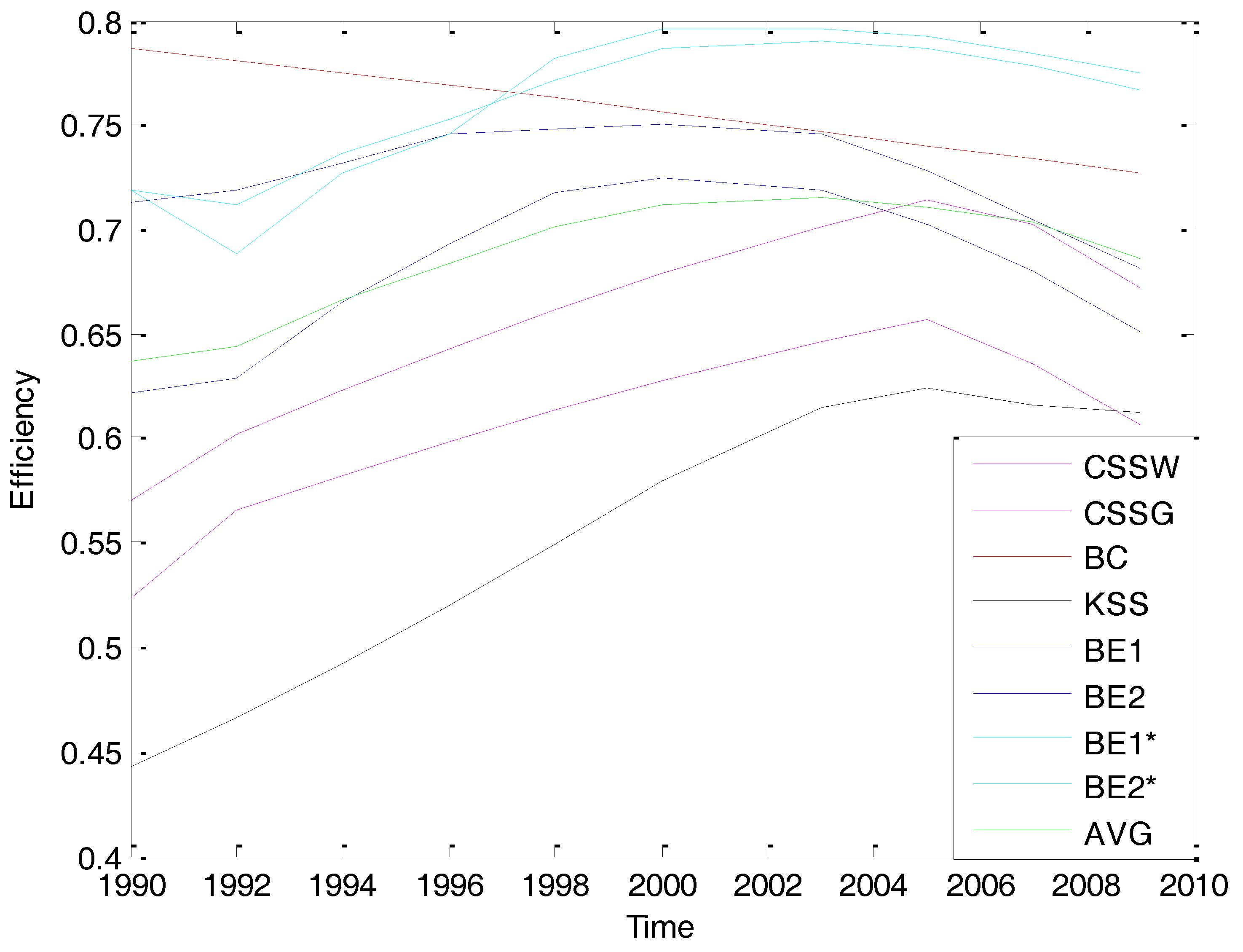
Table 1.
Monte Carlo simulations for DGP1.
| Mean Squared Error for the Individual Effects | |||||||||||||||
| n | T | BC | CSSW | CSSG | KSS | BE1 | BE2 | ||||||||
| 50 | 20 | 0.7284 | 0.0012 | 0.0012 | 0.0039 | 0.0053 | 0.0671 | ||||||||
| 50 | 0.9371 | 0.0005 | 0.0005 | 0.1255 | 0.0021 | 0.0323 | |||||||||
| 100 | 20 | 0.8222 | 0.0008 | 0.0008 | 0.0033 | 0.0031 | 0.0183 | ||||||||
| 50 | 0.8245 | 0.0003 | 0.0003 | 0.0220 | 0.0018 | 0.0115 | |||||||||
| 200 | 20 | 0.8451 | 0.0008 | 0.0008 | 0.0023 | 0.0027 | 0.0101 | ||||||||
| 50 | 0.8823 | 0.0003 | 0.0003 | 0.0021 | 0.0011 | 0.0083 | |||||||||
| Estimate and Standard Error for the Slope Coefficients | |||||||||||||||
| T = 20 | T = 50 | ||||||||||||||
| BC | CSSW | CSSG | KSS | BE1 | BE2 | BC | CSSW | CSSG | KSS | BE1 | BE2 | ||||
| n = 50 | |||||||||||||||
| EST1 | 0.5250 | 0.4961 | 0.4965 | 0.4954 | 0.4981 | 0.5017 | 0.5105 | 0.4991 | 0.4992 | 0.4999 | 0.5013 | 0.4998 | |||
| SE1 | 0.0130 | 0.0033 | 0.0032 | 0.0029 | 0.0057 | 0.0042 | 0.0073 | 0.0021 | 0.0020 | 0.0019 | 0.0035 | 0.0027 | |||
| EST2 | 0.4856 | 0.4949 | 0.4948 | 0.4919 | 0.4985 | 0.5020 | 0.4969 | 0.5048 | 0.5047 | 0.5053 | 0.5001 | 0.5002 | |||
| SE2 | 0.0139 | 0.0035 | 0.0033 | 0.0031 | 0.0055 | 0.0041 | 0.0073 | 0.0020 | 0.0020 | 0.0018 | 0.0032 | 0.0024 | |||
| n = 100 | |||||||||||||||
| EST1 | 0.4973 | 0.5018 | 0.5013 | 0.5045 | 0.5023 | 0.5002 | 0.4843 | 0.4999 | 0.4998 | 0.4991 | 0.4999 | 0.5001 | |||
| STD1 | 0.0099 | 0.0023 | 0.0022 | 0.0021 | 0.0032 | 0.0027 | 0.0066 | 0.0014 | 0.0014 | 0.0014 | 0.0023 | 0.0018 | |||
| EST2 | 0.5047 | 0.5009 | 0.5012 | 0.5022 | 0.5016 | 0.5001 | 0.4995 | 0.5001 | 0.5000 | 0.4990 | 0.5003 | 0.5001 | |||
| STD2 | 0.0098 | 0.0022 | 0.0022 | 0.0020 | 0.0032 | 0.0028 | 0.0066 | 0.0014 | 0.0014 | 0.0013 | 0.0022 | 0.0017 | |||
| n = 200 | |||||||||||||||
| EST1 | 0.4936 | 0.5013 | 0.5015 | 0.5009 | 0.5000 | 0.4981 | 0.5000 | 0.5007 | 0.5007 | 0.5000 | 0.5012 | 0.5001 | |||
| STD1 | 0.0071 | 0.0016 | 0.0016 | 0.0016 | 0.0027 | 0.0022 | 0.0042 | 0.0010 | 0.0010 | 0.0010 | 0.0019 | 0.0015 | |||
| EST2 | 0.4983 | 0.5016 | 0.5020 | 0.5019 | 0.5002 | 0.4993 | 0.5027 | 0.4972 | 0.4972 | 0.4969 | 0.5003 | 0.5004 | |||
| STD2 | 0.0071 | 0.0016 | 0.0016 | 0.0016 | 0.0027 | 0.0022 | 0.0042 | 0.0010 | 0.0010 | 0.0010 | 0.0018 | 0.0014 | |||
Table 2.
Monte Carlo simulations for DGP2.
| Mean Squared Error for the Individual Effects | |||||||||||||||
| n | T | BC | CSSW | CSSG | KSS | BE1 | BE2 | ||||||||
| 50 | 20 | 0.9202 | 0.1266 | 0.1266 | 0.0182 | 0.0071 | 0.0048 | ||||||||
| 50 | 0.9052 | 0.2996 | 0.2996 | 0.0238 | 0.0053 | 0.0025 | |||||||||
| 100 | 20 | 0.8588 | 0.4553 | 0.4553 | 0.0531 | 0.0040 | 0.0037 | ||||||||
| 50 | 0.9884 | 0.1065 | 0.1065 | 0.0046 | 0.0028 | 0.0013 | |||||||||
| 200 | 20 | 0.9183 | 0.6376 | 0.6375 | 0.0706 | 0.0022 | 0.0027 | ||||||||
| 50 | 0.9526 | 0.0616 | 0.0616 | 0.0028 | 0.0009 | 0.0008 | |||||||||
| Estimate and Standard Error for the Slope Coefficients | |||||||||||||||
| T = 20 | T = 50 | ||||||||||||||
| BC | CSSW | CSSG | KSS | BE1 | BE2 | BC | CSSW | CSSG | KSS | BE1 | BE2 | ||||
| n = 50 | |||||||||||||||
| EST1 | 0.4786 | 0.4857 | 0.4904 | 0.5059 | 0.5010 | 0.4993 | 0.4820 | 0.4811 | 0.4938 | 0.4972 | 0.5052 | 0.4983 | |||
| SE1 | 0.0460 | 0.0308 | 0.0298 | 0.0136 | 0.0262 | 0.0037 | 0.0243 | 0.0230 | 0.0227 | 0.0059 | 0.0177 | 0.0029 | |||
| EST2 | 0.4664 | 0.4414 | 0.4854 | 0.4599 | 0.5031 | 0.4992 | 0.4840 | 0.4660 | 0.4848 | 0.4988 | 0.5001 | 0.4999 | |||
| SE2 | 0.0491 | 0.0326 | 0.0314 | 0.0146 | 0.0261 | 0.0035 | 0.0241 | 0.0226 | 0.0225 | 0.0059 | 0.0174 | 0.0028 | |||
| n = 100 | |||||||||||||||
| EST1 | 0.4854 | 0.4818 | 0.4898 | 0.5065 | 0.4997 | 0.5002 | 0.5137 | 0.5360 | 0.5089 | 0.4950 | 0.5101 | 0.4987 | |||
| STD1 | 0.0200 | 0.0195 | 0.0188 | 0.0075 | 0.0163 | 0.0028 | 0.0415 | 0.0257 | 0.0254 | 0.0055 | 0.0128 | 0.0018 | |||
| EST2 | 0.5005 | 0.4996 | 0.5115 | 0.5101 | 0.4993 | 0.5001 | 0.4482 | 0.5283 | 0.5143 | 0.5127 | 0.5002 | 0.4992 | |||
| STD2 | 0.0198 | 0.0189 | 0.0186 | 0.0073 | 0.0164 | 0.0029 | 0.0415 | 0.0256 | 0.0254 | 0.0055 | 0.0130 | 0.0018 | |||
| n = 200 | |||||||||||||||
| EST1 | 0.5051 | 0.4995 | 0.5015 | 0.4864 | 0.4927 | 0.5013 | 0.4274 | 0.5097 | 0.4968 | 0.5018 | 0.5032 | 0.5011 | |||
| STD1 | 0.0169 | 0.0175 | 0.0171 | 0.0067 | 0.0120 | 0.0021 | 0.0527 | 0.0202 | 0.0200 | 0.0032 | 0.0078 | 0.0013 | |||
| EST2 | 0.4895 | 0.4898 | 0.5147 | 0.4951 | 0.4901 | 0.5020 | 0.3996 | 0.4930 | 0.5015 | 0.5042 | 0.5021 | 0.5031 | |||
| STD2 | 0.0170 | 0.0175 | 0.0171 | 0.0067 | 0.0121 | 0.0020 | 0.0531 | 0.0204 | 0.0202 | 0.0033 | 0.0077 | 0.0014 | |||
Table 3.
Monte Carlo simulations for DGP3.
| Mean Squared Error for the Individual Effects | |||||||||||||||
| n | T | BC | CSSW | CSSG | KSS | BE1 | BE2 | ||||||||
| 50 | 20 | 3.3477 | 0.8816 | 0.8816 | 0.0130 | 0.0244 | 0.0356 | ||||||||
| 50 | 3.3639 | 0.8469 | 0.8468 | 0.0082 | 0.0134 | 0.0152 | |||||||||
| 100 | 20 | 3.5102 | 0.8309 | 0.8303 | 0.0123 | 0.0116 | 0.0282 | ||||||||
| 50 | 3.7625 | 0.8357 | 0.8356 | 0.0072 | 0.0028 | 0.0053 | |||||||||
| 200 | 20 | 3.8433 | 0.8335 | 0.8333 | 0.0121 | 0.0083 | 0.0116 | ||||||||
| 50 | 3.8513 | 0.8393 | 0.8392 | 0.0063 | 0.0014 | 0.0019 | |||||||||
| Estimate and Standard Error for the Slope Coefficients | |||||||||||||||
| T = 20 | T = 50 | ||||||||||||||
| BC | CSSW | CSSG | KSS | BE1 | BE2 | BC | CSSW | CSSG | KSS | BE1 | BE2 | ||||
| n = 50 | |||||||||||||||
| EST1 | 0.5277 | 0.5250 | 0.4994 | 0.4989 | 0.5012 | 0.5002 | 0.4868 | 0.4871 | 0.4976 | 0.5005 | 0.4991 | 0.5001 | |||
| SE1 | 0.0188 | 0.0203 | 0.0197 | 0.0029 | 0.0081 | 0.0038 | 0.0122 | 0.0122 | 0.0120 | 0.0018 | 0.0041 | 0.0025 | |||
| EST2 | 0.4905 | 0.4998 | 0.5062 | 0.4930 | 0.4981 | 0.4997 | 0.5259 | 0.5255 | 0.5207 | 0.5052 | 0.4994 | 0.5003 | |||
| SE2 | 0.0198 | 0.0215 | 0.0207 | 0.0031 | 0.0078 | 0.0035 | 0.0121 | 0.0120 | 0.0119 | 0.0018 | 0.0042 | 0.0023 | |||
| n = 100 | |||||||||||||||
| EST1 | 0.4816 | 0.4768 | 0.4998 | 0.5030 | 0.4961 | 0.4992 | 0.4877 | 0.4863 | 0.4972 | 0.4986 | 0.4995 | 0.5002 | |||
| STD1 | 0.0132 | 0.0139 | 0.0134 | 0.0021 | 0.0058 | 0.0025 | 0.0076 | 0.0077 | 0.0076 | 0.0013 | 0.0022 | 0.0017 | |||
| EST2 | 0.4907 | 0.4816 | 0.5088 | 0.5028 | 0.4971 | 0.4985 | 0.5024 | 0.5118 | 0.5089 | 0.4993 | 0.4990 | 0.5004 | |||
| STD2 | 0.0131 | 0.0135 | 0.0133 | 0.0021 | 0.0057 | 0.0024 | 0.0076 | 0.0077 | 0.0076 | 0.0013 | 0.0023 | 0.0018 | |||
| n = 200 | |||||||||||||||
| EST1 | 0.5120 | 0.5103 | 0.5110 | 0.5016 | 0.5012 | 0.5011 | 0.4976 | 0.5012 | 0.4962 | 0.4999 | 0.4981 | 0.5052 | |||
| STD1 | 0.0088 | 0.0091 | 0.0089 | 0.0016 | 0.0042 | 0.0013 | 0.0055 | 0.0054 | 0.0054 | 0.0010 | 0.0015 | 0.0011 | |||
| EST2 | 0.4885 | 0.4892 | 0.5019 | 0.5029 | 0.5015 | 0.5014 | 0.4874 | 0.4883 | 0.4957 | 0.4973 | 0.4992 | 0.4994 | |||
| STD2 | 0.0088 | 0.0091 | 0.0089 | 0.0016 | 0.0041 | 0.0012 | 0.0055 | 0.0055 | 0.0054 | 0.0010 | 0.0016 | 0.0012 | |||
Table 4.
Monte Carlo simulations for DGP4.
| Mean Squared Error for the Individual Effects | |||||||||||||||
| n | T | BC | CSSW | CSSG | KSS | BE1 | BE2 | ||||||||
| 50 | 20 | 0.8042 | 0.2161 | 0.2161 | 0.0030 | 0.0130 | 0.0445 | ||||||||
| 50 | 0.9478 | 0.2056 | 0.2056 | 0.0890 | 0.0045 | 0.0141 | |||||||||
| 100 | 20 | 0.8770 | 0.1382 | 0.1382 | 0.0026 | 0.0112 | 0.0291 | ||||||||
| 50 | 0.8626 | 0.1337 | 0.1337 | 0.0193 | 0.0028 | 0.0055 | |||||||||
| 200 | 20 | 0.8764 | 0.1301 | 0.1301 | 0.0020 | 0.0098 | 0.0108 | ||||||||
| 50 | 0.9111 | 0.1445 | 0.1445 | 0.0015 | 0.0015 | 0.0021 | |||||||||
| Estimate and Standard Error for the Slope Coefficients | |||||||||||||||
| T = 20 | T = 50 | ||||||||||||||
| BC | CSSW | CSSG | KSS | BE1 | BE2 | BC | CSSW | CSSG | KSS | BE1 | BE2 | ||||
| n =50 | |||||||||||||||
| EST1 | 0.5521 | 0.5250 | 0.5329 | 0.4995 | 0.4922 | 0.4951 | 0.5031 | 0.4871 | 0.4901 | 0.4999 | 0.5051 | 0.5010 | |||
| SE1 | 0.0233 | 0.0203 | 0.0197 | 0.0030 | 0.0039 | 0.0031 | 0.0148 | 0.0122 | 0.0120 | 0.0019 | 0.0032 | 0.0025 | |||
| EST2 | 0.4788 | 0.4998 | 0.5014 | 0.4907 | 0.5011 | 0.4977 | 0.5201 | 0.5255 | 0.5246 | 0.5053 | 0.5001 | 0.5003 | |||
| SE2 | 0.0248 | 0.0215 | 0.0207 | 0.0031 | 0.0036 | 0.0032 | 0.0147 | 0.0120 | 0.0119 | 0.0018 | 0.0031 | 0.0028 | |||
| n = 100 | |||||||||||||||
| EST1 | 0.4732 | 0.4768 | 0.4713 | 0.5017 | 0.5001 | 0.5052 | 0.4720 | 0.4863 | 0.4867 | 0.4985 | 0.5003 | 0.5001 | |||
| STD1 | 0.0169 | 0.0139 | 0.0134 | 0.0022 | 0.0031 | 0.0027 | 0.0103 | 0.0077 | 0.0076 | 0.0014 | 0.0021 | 0.0017 | |||
| EST2 | 0.4880 | 0.4816 | 0.4836 | 0.5018 | 0.5000 | 0.5041 | 0.5077 | 0.5118 | 0.5117 | 0.4998 | 0.5002 | 0.5003 | |||
| STD2 | 0.0167 | 0.0135 | 0.0133 | 0.0021 | 0.0032 | 0.0025 | 0.0103 | 0.0077 | 0.0076 | 0.0014 | 0.0020 | 0.0015 | |||
| n = 200 | |||||||||||||||
| EST1 | 0.5029 | 0.5103 | 0.5112 | 0.5011 | 0.5032 | 0.5001 | 0.4891 | 0.5012 | 0.5012 | 0.5003 | 0.4991 | 0.5002 | |||
| STD1 | 0.0116 | 0.0091 | 0.0089 | 0.0016 | 0.0028 | 0.0020 | 0.0069 | 0.0054 | 0.0054 | 0.0010 | 0.0018 | 0.0014 | |||
| EST2 | 0.4892 | 0.4892 | 0.4934 | 0.5021 | 0.5013 | 0.5020 | 0.4940 | 0.4883 | 0.4886 | 0.4970 | 0.4987 | 0.5013 | |||
| STD2 | 0.0116 | 0.0091 | 0.0089 | 0.0016 | 0.0025 | 0.0022 | 0.0070 | 0.0055 | 0.0054 | 0.0010 | 0.0017 | 0.0013 | |||
Table 5.
Estimation results.
| Model | BC | CSSW | CSSG | KSS | BE1 | BE2 | BE1* | BE2* |
|---|---|---|---|---|---|---|---|---|
| PFA | −0.1267 | −0.1067 | −0.1243 | −0.0448 | −0.1221 | −0.0505 | −0.0972 | −0.0555 |
| NOE | −0.1518 | −0.2750 | −0.2731 | −0.2195 | −0.1520 | −0.0666 | −0.1145 | −0.0424 |
| PF | −0.1088 | −0.0571 | −0.0628 | −0.0679 | −0.0570 | −0.1387 | −0.0930 | −0.1003 |
| SA | −0.3058 | −0.1026 | −0.1413 | −0.1289 | −0.1700 | −0.3042 | −0.1030 | −0.2542 |
| CD | −0.2938 | −0.2422 | −0.2492 | −0.1526 | −0.2363 | −0.2867 | −0.1541 | −0.2012 |
| DD | −0.0295 | −0.0055 | −0.0297 | −0.0321 | −0.0259 | −0.0636 | −0.0715 | −0.0335 |
| REL | 0.6302 | 0.6267 | 0.6254 | 0.5468 | 0.6182 | 0.6099 | 0.4103 | 0.4242 |
| CIL | 0.2674 | 0.2116 | 0.2053 | 0.3200 | 0.2300 | 0.2630 | 0.2415 | 0.2208 |
| CL | 0.1024 | 0.1617 | 0.1693 | 0.1332 | 0.1518 | 0.1271 | 0.1013 | 0.1212 |
| RTS | 1.0165 | 0.7891 | 0.8804 | 0.6459 | 0.7634 | 0.9102 | 0.6333 | 0.6871 |
| Avg.TE | 0.7576 | 0.6094 | 0.6608 | 0.5552 | 0.4584 | 0.6937 | 0.7944 | 0.7889 |
Table 6.
Estimated efficiencies (evaluated at means) and Bayes factor in favor of endogeneity.
| Without Endogeneity | With Endogeneity | BF† | |||
|---|---|---|---|---|---|
| BE1 | BE2 | BE1* | BE2* | ||
| 1990 | 0.6216 | 0.7125 | 0.7189 | 0.7192 | 3.672 |
| 1992 | 0.5915 | 0.7317 | 0.6179 | 0.7003 | 3.855 |
| 1994 | 0.6718 | 0.7106 | 0.7283 | 0.7146 | 3.781 |
| 1996 | 0.7103 | 0.7325 | 0.7781 | 0.7613 | 4.038 |
| 1998 | 0.7317 | 0.7716 | 0.7925 | 0.7845 | 4.129 |
| 2000 | 0.7612 | 0.7815 | 0.8105 | 0.8006 | 4.217 |
| 2003 | 0.7120 | 0.7451 | 0.8023 | 0.7942 | 5.333 |
| 2005 | 0.7101 | 0.7222 | 0.7945 | 0.7943 | 5.885 |
| 2007 | 0.6787 | 0.7104 | 0.7824 | 0.7745 | 6.452 |
| 2009 | 0.6513 | 0.6817 | 0.7748 | 0.7663 | 6.812 |
†BF calculation, see Perrakis et al. (2014).
© 2017 by the authors. Licensee MDPI, Basel, Switzerland. This article is an open access article distributed under the terms and conditions of the Creative Commons Attribution (CC BY) license (http://creativecommons.org/licenses/by/4.0/).
Share and Cite
MDPI and ACS Style
Liu, J.; Sickles, R.C.; Tsionas, E.G. Bayesian Treatments for Panel Data Stochastic Frontier Models with Time Varying Heterogeneity. Econometrics 2017, 5, 33. https://doi.org/10.3390/econometrics5030033
AMA Style
Liu J, Sickles RC, Tsionas EG. Bayesian Treatments for Panel Data Stochastic Frontier Models with Time Varying Heterogeneity. Econometrics. 2017; 5(3):33. https://doi.org/10.3390/econometrics5030033
Chicago/Turabian StyleLiu, Junrong, Robin C. Sickles, and E. G. Tsionas. 2017. "Bayesian Treatments for Panel Data Stochastic Frontier Models with Time Varying Heterogeneity" Econometrics 5, no. 3: 33. https://doi.org/10.3390/econometrics5030033
Note that from the first issue of 2016, this journal uses article numbers instead of page numbers. See further details here.