
Building News Measures from Textual Data and an Application to Volatility Forecasting


1
Department of Statistical Sciences, University of Padova/via Cesare Battisti, 241, 35121 Padova PD, Italy
2
Department of Economics and Management, University of Padova/via del Santo, 33, 35123 Padova PD, Italy
*
Author to whom correspondence should be addressed.
Econometrics 2017, 5(3), 35; https://doi.org/10.3390/econometrics5030035
Submission received: 5 April 2017
/
Revised: 2 August 2017
/
Accepted: 14 August 2017
/
Published: 19 August 2017
(This article belongs to the Special Issue Big Data in Economics and Finance)
Abstract
:We retrieve news stories and earnings announcements of the S&P 100 constituents from two professional news providers, along with ten macroeconomic indicators. We also gather data from Google Trends about these firms’ assets as an index of retail investors’ attention. Thus, we create an extensive and innovative database that contains precise information with which to analyze the link between news and asset price dynamics. We detect the sentiment of news stories using a dictionary of sentiment-related words and negations and propose a set of more than five thousand information-based variables that provide natural proxies for the information used by heterogeneous market players. We first shed light on the impact of information measures on daily realized volatility and select them by penalized regression. Then, we perform a forecasting exercise and show that the model augmented with news-related variables provides superior forecasts.
JEL Classification:
C55; C52; C58; C221. Introduction
Traditional “efficient markets” thinking suggests that asset prices should completely and instantaneously reflect movements in underlying fundamentals, while an opposite view indicates that asset prices and fundamentals are continuously disconnected. One hypothesis that explains the success of the GARCH class of models is the mixture of distributions hypothesis (MDH). (See Clark 1973; Epps and Epps 1976; Tauchen and Pitts 1983; and Lamoureux and Lastrapes 1990, among many others.) According to the MDH, a serially correlated mixing variable that measures the rate at which information arrives to the market explains the GARCH effects on asset returns. The validity of the MDH remains an open debate; there is no agreement about how quickly and in what form responses to news occur. We shed light on the link between news information and volatility, focusing on three questions: What is the relative importance of types of news? Are investors more influenced by the volume of information or by variations if it? Do news and an index of investors’ attention help to forecast volatility?
Our first contribution is to create an extensive and innovative database that contains information useful in answering the three questions. From two news providers, Factset-StreetAccount and Thomson Reuters-Thomson One, we retrieve news stories and earnings announcements of the S&P 100 constituents, along with ten macroeconomic announcements. Both news providers assign news stories a topic—Thomson Reuters also gives its news stories a level of importance—while earnings and macro-announcements report both released figures and consensus forecasts, allowing diversions from expectations to be computed. In addition, we gather Google Trends1 information about the assets and use them as a proxy for retail investors’ attention. Google restricts access to daily data for intervals longer than ten months but allows daily data to be gathered for shorter intervals. Exploiting the series of daily data associated with each month and the series of monthly data associated with the whole sample, we reconstruct the daily relative search volume for the whole sample. The collected news reports are dated with to-the-minute precision, while Google Trends are aggregated by day, so the dataset has to-the-minute precision for news and daily precision for Google Trends. The sample contains data for the ten-year period from February 2005 to February 2015.
As a second contribution, we detect the sentiment of news stories using the sentiment-related word lists developed by Loughran and McDonald (2011) and introduce a set of negations, both with the aim of creating a method that can be used to extract the sentiment of a financial text with more confidence and independent of its type, length, and audience.
Our third contribution is to propose a set of news measures that provide natural proxies for retail investors’ attention and for the information heterogeneous market players use. This study goes beyond how information has been used so far: starting from the reasoning that investors’ perception and, as a consequence, their reaction to news disclosures can differ based on how information varies over time and the reasoning that investors digest and react to news at differing speeds, we look at how the information stream fluctuates over the day and across days, weeks, and months. We end with a large set of news measures, each representing a different type of information that can cause a different market reaction.
As final contribution, we shed light on the impact of news on volatility and address the three questions posed above using the information-related variables we develop. We perform an application using the database to explain realized volatility and selecting the most important indicators with LASSO (least absolute shrinkage and selection operator), an estimation method for linear models that is commonly employed in big data analysis which performs variable selection and shrinks coefficients. Then we employ news and Google Trends to forecast volatility in an out-of-sample analysis.
Empirical analyses favor the MDH and show that earnings announcements and news stories are the most important drivers of daily realized volatility, followed by macroeconomic news and Google Trends, and that earnings and upgrades/downgrades are the topics of news stories that are most relevant to explaining volatility. In addition, the analyses show that it is important both to look at variations of the volume of information across time and to build measures based on the aggregation of information over various time horizons since the measures imply varying reactions from market players. By including news-based information, we can improve volatility forecasting substantially.
2. Literature Review
2.1. Mixture of Distributions Hypothesis
The MDH is a classic topic in the finance literature. Clark (1973), Epps and Epps (1976), and Tauchen and Pitts (1983) use different approaches to test the relationship between returns variance and trading volume for the same interval of time. Lamoureux and Lastrapes (1990) show that trading volume can be used as a proxy for information arrival, that it has significant explanatory power regarding the variance of the daily returns, and that ARCH effects tend to disappear when volume is included in the variance equation. More recently, Kalev et al. (2004) find results that are consistent with the MDH by employing firm-specific announcements and lagged volume as a proxy for information flows and investigating the information-volatility relationship using high-frequency data from the Australian Stock Exchange. Martens et al. (2009) evaluate the forecasting performance of time series models for realized volatility and account for the effects of macroeconomic news announcements, arguing that allowing volatility to differ on days that contain news releases can disentangle calendar and announcement effects. McMillan and García (2013) forecast intra-day volatility for the IBEX 35 Index futures using volume and the number of transactions as proxies for information flows and show that introducing the proxy improves the volatility forecast for several volatility models at various frequencies. Zhang et al. (2014) employ the number of news stories that appeared in Baidu News2 as a proxy for information arrival and use a sample of SME Price Index3 in China to validate the MDH. Their empirical results reveal a positive impact of internet information on the conditional volatility of stock returns. This link has also been documented for the US stock market (Kim and Kon 1994; Gallo and Pacini 2000), the UK stock market (Omran and McKenzie 2000), and the Australian stock market (Brailsford 1996).
More generally with regard to the relationship between news flows and asset price dynamics, the last few decades of research have produced a tremendous number of empirical studies, but these studies have by no means reached consensus. While some of these papers focus on the impact of macroeconomic news, others explore the idea that assets react to firm-specific news releases.
2.2. Macroeconomic News
The finance literature began analyzing the relationship between news and market movements with studies like Cutler et al. (1989), who report a faint relationship among macroeconomic news, world political events, and stock market activity, and Schwert (1989), who finds weak evidence that macroeconomic volatility can explain stock return volatility. A stream of the literature addresses the volatility reaction to news released on announcement days, focusing on the dynamics of conditional volatility based on the ARCH/GARCH framework introduced by Engle (1982) and Bollerslev (1986). For example, Li and Engle (1998) compare the degree of persistence associated with scheduled macroeconomic announcement days and non-announcement days in the Treasury futures market and find heterogeneous persistence. Jones et al. (1998) present a similar analysis for the Treasury bond market, and show U-shaped day-of-the-week effects and calm-before-the-storm effects for bond returns’ volatility. In contrast to Li and Engle (1998), Jones et al. (1998) find that announcement-day shocks do not persist at all, as they are purely transitory. Flannery and Protopapadakis (2002) also use a GARCH model to detect a consistent influence of monetary and macroeconomic variables on stock market indices. Bomfim (2003), whose work is based on Jones et al. (1998)’s framework, examines the effect of monetary policy announcements on the volatility of stock returns, finding that unexpected monetary policy decisions tend to boost volatility significantly in the short run. Using conditional variance modelling, Janssen (2004) demonstrates an intertemporal relationship between the arrival of public information (measured as the daily number of economic news headlines) and volatility persistence of US stocks, Treasury bills, bonds, and the dollar. Engle and Rangel (2008) find a strong relationship between the low-frequency component of market volatility, represented by an exponential spline, and macroeconomic variables like inflation, growth, and macroeconomic volatility. Vrugt (2009) analyzes the impact of US and Japanese macroeconomic news on stock market volatility in Japan, Hong Kong, South Korea, and Australia and employ a GARCH model that allows for multiplicative announcement effects and asymmetries to find that overnight conditional variances are higher on announcement days than on days before and after announcements, especially for US news, while the impact of announcements on implied volatilities is weak. Brenner et al. (2009) find that US macroeconomic information drives the level, volatility, and co-movement of the US stock, Treasury, and corporate bond markets. Hautsch et al. (2011) find that the arrival of macroeconomic news has an impact on the bid and ask dynamics of the German Bund futures. Rangel (2011) examines the effect of macroeconomic releases on stock market volatility through a Poisson-Gaussian-GARCH process with time-varying jump intensity, which is allowed to respond to information, and finds that macroeconomic surprises impact both volatility and jump intensity. Birz and Lott (2011) choose newspaper stories about GDP and unemployment as a measure of news and find that macroeconomic news affects S&P 500 returns. Savor and Wilson (2013) document higher average excess market returns on days with important macroeconomic news releases compared to non-announcement days.
2.3. Firm-Specific News and Sentiment
With regard to firm-specific news, Mitchell and Mulherin (1994), Berry and Howe (1994) and Roll (1988) are among the first to report a weak relationship between stock market activity and news. Kalev et al. (2004) document a positive relationship between the number of intraday news articles and the Australian stock market volatility, and in another intraday study Busse and Green (2002) consider the impact of news released via television on more than 300 stocks to test market efficiency. However, both studies show that the impact of news on intraday trading activity is weak, that it disappears altogether if earnings announcements are discarded, and that news stories have to be aggregated to reduce the influence of noisy and non-informative news. Fang and Peress (2009) explore news coverage and predictability of returns and find that stocks with no media coverage earn higher returns than do stocks with high media coverage. Baklaci et al. (2011) explore the relationship between intraday firm-specific news announcements and return volatility in the Turkish stock market and find that the persistence of volatility diminishes with the inclusion of news, suggesting that news is rapidly incorporated into prices.
Several studies investigate the relationship between news sentiment and changes in asset price dynamics. Antweiler and Frank (2004) are the first to develop news sentiment measures to explain stock returns. Using a Naive Bayes algorithm based on the number of times certain words occur, they infer trading signals from posts on internet message boards and find that, while such signals can predict market volatility, their effect on stock returns is small. Zhang et al. (2012) incorporate several methodological improvements and create news sentiment indices that are significant directional indicators. Tetlock (2007) undertakes the so-called bag-of-words approach, which has become widespread in the literature. This approach consists of building lists (bags) of words and associating each list with a category (e.g., positive or negative). Classifying words based on categories from the Harvard Psychosocial Dictionary, Tetlock quantifies optimism and pessimism from the Wall Street Journal’s “Abreast of the Market” column and reports that high levels of media pessimism predict declining market prices, which are followed by price reversals. Using a similar technique, Tetlock et al. (2008) use the Harvard IV-4 Psychological Dictionary and find that the fraction of negative words in Dow Jones News Service and Wall Street Journal stories forecasts firm earnings because the linguistic content of news messages captures the hard-to-quantify aspects of fundamentals that are quickly incorporated into stock prices. Thanks to recent advances in technology, software packages like Reuters NewsScope Sentiment Engine, the more recent Thomson Reuters News Analytics4, and Ravenpack News Analytics5 have been developed. These packages use advanced algorithms and assign sentiment indicators to firm-specific newswire releases, enabling investors who pay for the service to employ “real-time” trading signals from textual analysis in quantitative trading strategies. Gloß-Klußmann and Hautsch (2011) employ the trading signals from Reuters NewsScope Sentiment Engine to find that high-frequency responses in market activity and volatility are significant, especially after the release of intraday company-specific news, and that classifying news according to relevance helps to filter noise and identify significant effects. Using sentiment scores generated at high frequency by RavenPack News Analytics, Ho et al. (2013) find a significant impact of firm-specific news sentiment on intraday volatility persistence, even after controlling for the potential effects of macroeconomic news. Firm-specific news sentiment apparently accounts for a greater proportion of overall volatility persistence than macroeconomic news sentiment does, and negative news has a greater impact on volatility than positive news does. Riordan et al. (2013) suggest that negative newswire messages from Reuters NewsScope Sentiment Engine, compared to positive ones, are associated with higher adverse selection costs, are more informative, and have a more significant impact on high-frequency asset price discovery and liquidity. Smales (2015) use Thomson Reuters News Analytics sentiment scores to create aggregate daily news sentiment indicators and find that positive and negative news result in above and below average returns, respectively, and that neutral news days are indistinguishable from days without news. Allen et al. (2017) use the Thomson Reuters News Analytics data set to construct a series of daily sentiment scores for the Dow Jones Industrial Average (DJIA) stock index component companies, and study the relationship between these financial news sentiment scores and the stock prices of these companies using entropy metrics, which permit an analysis of the amount of information within the sentiment series, its relationship to the DJIA and an indication of how the relationship changes over time. Allen et al. (2015a, 2015b) explore the impact of the Thomson Reuters News Analytics series on the DJIA constituents asset pricing and volatility. The relation between news and price dynamics has been studied for other types of assets, as well. For instance, Borovkova and Mahakena (2015) investigate the impact of news sentiment on returns, price jumps and volatility of natural gas futures. They find significant relationships between news sentiment and the dynamic characteristics of natural gas futures prices and document, among other findings, an asymmetric effect of (positive vs negative) news on volatility. In the books Mitra and Mitra (2011) and Mitra and Yu (2016), several articles deal with many related research questions. In the field of bag-of-words methods in financial contexts, Loughran and McDonald (2011) show that word lists developed for other disciplines misclassify common words in financial texts and develop alternative positive and negative word lists and four other word lists that reflect tone in financial texts. They show that the proportion of negative words in annual 10-Ks reports6 is associated with lower returns.
Differently from previous studies that use or focus on only macroeconomic or firm-specific information, Bajgrowicz et al. (2016) consider macro, pre-scheduled company-specific announcements and stories from news agencies like Reuters and Dow Jones News Service and relate them to jumps in the US stock market.
2.4. Google Trends
Quantitative data on internet use will soon be an invaluable source for economic analysis since they capture investors’ attention and information demand. Ginsberg et al. (2009), in the first article to use Google data, estimate the weekly influenza activity in the US using an index of health-seeking behavior that is equal to the incidence of influenza-related internet queries. Since then, the use of internet search data has been extended rapidly in estimating economic variables. For instance, Baker and Fradkin (2011) develop a job-search activity index to analyze the reaction of job-search intensity to changes in the duration of unemployment benefits in the US, and D’Amuri and Marcucci (2012) suggest that the Google index (GI), based on internet job searches performed through Google, is the best leading indicator of the US monthly unemployment rate. Recent studies have shown that online search activity is also associated with volatility and returns in the financial, commodity, and exchange-rate markets. (See Da et al. (2011) and Vlastakis and Markellos (2012) for individual stocks; Andrei and Hasler (2015), Dimpfl and Jank (2016), and Hamid and Heiden (2015) for stock indexes; Vozlyublennaia (2014) for stock and bond indices, gold, and crude oil; Da et al. (2015) for stock indices, the VIX volatility index, and equity and Treasury bonds mutual funds; Guo and Ji (2013) for crude oil; and Smith (2012) and Goddard et al. (2015) for exchange rates.)
3. Database Construction
Our first contribution lies in the extraction of information collected from two news providers, FactSet-StreetAccount and Thomson Reuters-Thomson One, and from Google Trends. Here we describe our novel dataset and the procedures used to extract the data.
3.1. Dataset
A large set of firm-specific and macroeconomic news is available from the two news providers FactSet-StreetAccount and Thomson Reuters-Thomson One. As Gloß-Klußmann and Hautsch (2011) point out, recording and analyzing the overall news flow for a specific asset is challenging since the amount of news, the number of news sources, and the speed of information dissemination are all rapidly increasing. Because of the huge amount of information published in all modern media, news are overlaid with substantial noise from irrelevant information. Since we rely on two professional news providers that provide only firm-specific news classified by their professionals as relevant to the firm, we assume that relevant news stories are effectively disentangled from irrelevant ones and that the impact of noise is adequately reduced. Our approach differs substantially in this regard from work that analyzes newspapers articles that are not selected a priori.7
StreetAccount, owned by the financial data and software company FactSet, is a news provider that supplies investment professionals with news summaries. StreetAccount data includes real-time company updates, portfolio and sector filtering, email alerts, and market summaries. Content can be customized for portfolio, index, sector, market, time of day (e.g., overnight summaries), and category (e.g., top stories, market summaries, economic stories, M&A stories). Writers, all of whom are financial professionals, include former portfolio managers, traders, analysts, and economists who use their collective market expertise to scan all possible sources for corporate news and report only those stories that they consider new and material. Comprehensive U.S. and European company coverage and coverage of a smaller but relevant list of Canadian and Asia Pacific companies extend to thousands of companies. Firm-specific and macroeconomic news are available in StreetAccount.
Thomson Reuters is a world-leading source of information for businesses and professionals, and Thomson One, one of its core products, is a database that provides financial market news from Reuters and leading third-party sources. Thomson One data results from the incorporation of 400 real-time global sources and newswires and more than 6,000 global and regional sources, including The Economist, Barron’s, Le Monde, The Washington Post, PR Newswire, Business Wire, and The Wall Street Journal. Comprehensive global coverage of 57,000 publicly listed companies spanning more than 120 markets tracked and corresponding to 99 percent of global market capitalization includes the constituents of all major indices and extends to the frontier/emerging markets of Central and Eastern Europe, Asia, the Middle East, and Africa. Firm-specific news is available in a variety of formats, each corresponding to a type of information: Significant Developments, Company Events, and Earnings Surprises. Macroeconomic news is available as well from Thomson One.
Following the growing popularity of the internet as a search tool, the use of such sources as Google to find information on a certain stock seems to be closely linked to stock market participation. (See, e.g., Preis et al. (2010).) However, as Da et al. (2011) point out, Google is likely to be representative of general internet search behavior, so the quantity of queries for a term is a measure for retail investors’ activity, rather than for professional investors’ activity. Therefore, we use Google Trends’ public data as a proxy for retail investors’ attention.
We gather news about ten US macroeconomic indicators and firm-specific news and Google Trends for the S&P 100 Index companies since they are highly capitalized and attention-grabbing companies. We excluded from the database: (1) stocks whose news stories were not available from either provider for the period February 2005–February 2015, and (2) stocks that entered the S&P 100 Index or were created after February 2005. Eleven stocks were excluded, and the remaining eighty-nine stocks are listed in Table A1 in Appendix A.
The information that constitutes the database can be classified into five types:
- StreetAccount news stories: firm-specific news stories released by StreetAccount
- Thomson Reuters news stories: firm-specific news stories released by Thomson Reuters
- Earnings announcements: firm-specific EPS earnings per share (announcement and forecast) released by StreetAccount
- Macro-announcements: ten macroeconomic indicators (announcement and forecast) released by Thomson Reuters
- Google Trends: firm-specific relative indicators of internet search volume available from Google
Firm-specific StreetAccount news stories include trading-floor conjectures, court rulings, FDA and EU drug approvals, FTC antitrust decisions, SEC filings, brokerage firm upgrades and downgrades, newspaper and television stories, stories released by social media, and company press releases, including perspectives, corporate conference calls, and presentations. News are classified along eleven topics, which are listed in Table A2 in Appendix A. News are filtered for relevancy and redundancy so each news story is included only once.
Firm-specific Thomson Reuters news stories are available from Significant Developments, a news analysis, tagging, and filtering service of Thomson One that screens press releases and provides concise summaries and categorizations of important company events on a near real-time basis. Customized reports can be created for a portfolio of companies, regions, industries, and news topics. Each story is organized into one or more of thirty-six topics and is given one of four levels of significance/importance: low, medium, high, and top, where each level implies a filter which eliminates all news stories with a lower significance; for instance, low corresponds to all news stories, while medium corresponds to news stories from medium to top. The thirty-six topics are listed in Table A2 in Appendix A. Assignment of degree of significance is based on the expected effect that the event will have on the company’s operational and/or financial performance. As for StreetAccount news, Thomson Reuters news stories are also filtered for relevance and redundancy. Firm-specific company events are also available from Thomson One and consist of a comprehensive list of current and past events—primarily earnings releases, conference calls, news conferences, and shareholders’ meetings. While they are not categorized by topic, they are short descriptions of the events that do not allow sentiment to be extracted. For these reasons we do not use company events to construct news measures, but they are part of our database and are reported here.
Firm-specific earnings announcements incorporate both the company’s reported actual EPS and the consensus forecast figure, given as the mean of a set of surveys at the time of reporting, so investors and analysts can determine whether the company has met, exceeded, or fallen short of the street’s expectations. Earnings announcements are recovered by StreetAccount news stories that contain the quarterly EPS announcements and their consensus forecast, which we compare to compute earnings surprises. Thomson One reports earnings surprises too; although the figures are highly reliable since they are computed by the provider, data are available with day precision instead of minute precision and are limited to the period July 2013 – June 2015. As a consequence of these limitations, we do not use Thomson Reuters earnings surprises in this study.
Ten US macroeconomic indicators are available from Thomson One, and they are listed in Table 1.
Google Trends summarizes the searches performed through the Google website and shows how many web searches have been done for a particular keyword in a particular period of time in a particular geographical area relative to the total number of web searches performed through Google in the same period and area. Absolute values of the index are not publicly available since Google normalizes the index to 100 in the period in which it reaches the maximum level. Data are gathered using IP addresses only if the number of searches exceeds a certain threshold. Repeated queries from a single IP address within a short time are eliminated. Google Trends have been available almost in real time since the end of January 2004. For each stock, we look at the number of search queries for the name of the company but do not include search queries for the company’s products or other related expressions since it is likely that investors search for the company’s name when they look for information about it. We also exclude search queries for tickers since, in many cases, they correspond to acronyms for other institutions or have other meanings. Google restricts the access to daily data for intervals longer than ten months but allows daily data (relative to the maximum) to be gathered for shorter intervals. For the ten-year period, we reconstruct the daily search volume for the whole sample from the set of the daily series for each month and the monthly aggregated series for the whole sample, following a procedure detailed in Section 5.3.
The dataset’s time range is 4 February 2005 to 25 February 2015, and all data is available with minute precision, except for Google Trends, which are daily.
News is available in various data formats, depending on the provider. Using the software , we extracted from each news story a set of elements that depend on the type of news, its data format, and its provider. For StreetAccount and Thomson Reuters news stories we obtain stock, date with minute precision time, headline, topic (also importance for Thomson Reuters news stories), and text. For company events we derive stock, date, time, and event description. For earnings announcements we extrapolate stock, date, time, actual EPS, and consensus forecast EPS. For macro-announcements we isolate type of macro-indicator (e.g., GDP), date, time, actual figure, and consensus forecast. With regard to Google Trends, we collect for each stock the set of the daily series for each month and the monthly aggregated series for the whole sample.
3.2. Topics and Importance for News Classification
StreetAccount news stories are classified into six of the eleven available topics—earnings-related, litigation (court disputes), M&A, newspapers, regulatory, and upgrades/downgrades—or all (all news, no filter by topic). The other topics were discarded because they lacked in either importance or frequency.8
Thomson Reuters news stories are classified by both importance and topic. We use all four levels of importance (low, medium, high, and top) and build six topics from the thirty-six available: all, earnings pre-announcements, financial, litigation, M&A, and regulatory/company investigation (events concerning regulatory agencies, internal investigations, and any type of charges brought by regulatory bodies). The earnings pre-announcements topic merges three topics: positive earnings pre-announcements (higher than expected), negative earnings pre-announcements (lower than expected), and other earnings pre-announcements (neutral with respect to expectations). The financial topic merges equity issues, bond issues, share repurchases, and equity investments, all of which are events that have an impact on the company’s balance sheet. The other topics were discarded for reasons similar to those that led to our discarding some of StreetAccount news’ topics. By jointly exploiting topics and importance, we get (n. importance) × (n. topics) = 4 × 6 = 24 classifications for Thomson Reuters news stories.
Topics from different providers that appear to have the same meaning usually have similarities but can also differ significantly because they depend on the criteria the analysts use for news categorization, and topics often have different meanings. For instance, StreetAccount’s earnings-related news is a more broad concept than Thomson Reuters’ earnings pre-announcements, since the former is comprehensive of earnings pre-announcements released by the company, consensus forecasts released by the provider, and EPS announcements, while the latter consists only of the company’s earnings pre-announcements. As another example, StreetAccount’s regulatory news topic apparently does not include company-internal investigations, unlike Thomson Reuters’ regulatory/company investigation.
Table 2 lists the topics that are included in our dataset for each data provider.
3.3. News stories’ Summary Stats and Provider Comparison
Table 3 presents the summary statistics of the basic variables number of news stories per day and number of words per day; for StreetAccount’s news stories the all topic, and for Thomson Reuters news stories the all topic with low importance. (Low importance means that there is no filter; that is, all news categorized from low to top is included.) The tables report the cross-sectional median of min, 5% quantile, median, 95% quantile, max, mean, standard deviation for each measure. StreetAccount releases more news than Thomson Reuters on average—more than one news story every five days versus one news story every ten days. StreetAccount and Thomson Reuters news stories have, roughly, the same length.
In order to understand to what degree the information supplied by the two providers is similar, we compute, for a series of topics (pooling all stocks), the ratio between the number of days in which both providers report at least one news story and the number of days in which at least one provider reports at least one news story, naming the result Coincident/Total Ratio. The higher the ratio, the greater the similarity of the information released by the two providers. We compare the topics all (no filter), earnings (StreetAccount’s earnings-related vs. Thomson Reuters’ earnings pre-announcements), litigation, M&A, and regulatory (StreetAccount’s regulatory vs. Thomson Reuters’ regulatory/company investigation). Table 4 reports the Coincident/Total Ratio, the percentage of days with at least one news release by StreetAccount, and the percentage of days with at least one news release by Thomson Reuters. Even when the news occurrence is aggregated on a daily level, it is clear that StreetAccount and Thomson Reuters supply different information. Therefore, we use news stories released by both providers in the rest of this study.
4. Sentiment Detection
Our second contribution consists of detecting the sentiment of news stories. Sentiment indicates whether the content of a document—in our case, a news story—is good, bad, or neutral in relation to the issue it addresses. We use the sentiment-related word lists developed by Loughran and McDonald (2011) and introduce a set of negations, with the aim of creating a method for extracting the sentiment of a financial text with more confidence and independent of its type, length, and audience.
Loughran and McDonald (2011) develop six word lists (negative, positive, uncertainty, litigious, strong modal, and weak modal) and show that a higher proportion of negative words is associated with lower returns. Their lists are tailored for financial texts; for example, they do not contain words like liability, earnings, and tax, which are expected to appear in both positive and negative contexts. The authors account for negation with six words (no, not, none, neither, never, and nobody), but only if they precede words that are classified as positive. The methodology is applied to US companies’ 10-K filings and these texts have a formal tone and are unlikely to contain many negations. We deal instead with news created by news providers, which we expect to be less limited in the use of language compared to company filings of 10-Ks. Loughran and McDonald (2011)’s procedure is not adequate for extracting the sentiment of news stories from news providers because, unlike 10-Ks that are given to the SEC, news stories do not necessarily have a formal tone; in addition, 10-Ks are long enough that, if negated words occur and their sentiment is incorrectly identified, the effect is negligible in the whole, long document. We deal, instead, with news stories that are seldom longer than a few dozen words.
Negations can appear in various forms and can invert the meaning of whole phrases, as well as single words. The phrase whose meaning is changed is called the negation scope. Negations can also flip the meaning of sentences, as in “the company has invented a new product for the first and last time.” Identifying negation scopes, implicit negations, and linguistic peculiarities like sarcasm and irony still presents many problems. Approaches like heuristic rules and machine-learning that perform natural language processing can bring significant improvements, but they are out of the scope of the present work.
Remaining in the field of the bag-of-words and avoiding the numerical complexities implied by the aforementioned approaches, we invert the sentiment each time a word, whether positive or negative, is preceded by a negation; and in place of the short negations list of six single words, we use twenty-eight single words, twenty-four sequences of two words, and six sequences of three words. We believe that this modification allows the sentiment of a financial text to be extracted with more confidence and independent of its type, length, and audience:
- single words: no, not, none, never, nothing, nobody, nowhere, neither, nor, hardly, scarcely, seldom, barely, few, little, rarely, instead, can’t, cannot, don’t, doesn’t, didn’t, mustn’t, won’t, despite, overly, too, less
- two-word sequences: can not, do not, did not, short of, not every, not all, not much, not many, not always, not so, instead of, far from, not to, never to, no way, out of, not very, not enough, too few, too little, no big, not big, no significant, not significant
- three-word sequences: not at all, by no means, in no way, in place of, in spite of, in lieu of
The procedure we develop works as follows:
- Positive words are given a value of 1 and negative words a value of ; the value is inverted in case of negation.
- The values of all words with a sentiment are summed to get the sentiment sum (Sent_Sum):where i is the word index, N is the number of words with a sentiment in a text, and is the sentiment of the word indexed by i.
- Sent_Sum is divided by the number of words with a sentiment to obtain a standardized quantity that we call relative sentiment (Rel_Sent) and that is between −1 and 1 by construction:
- If Rel_Sent is larger than 0.05 or smaller than , we associate a positive (1) or a negative sentiment () to the news, respectively; otherwise a neutral sentiment (0) is given. News sentiment is therefore neutral when a significant number of positive and negative words are detected and their proportion is roughly the same:
Different from the mainstream of text-analysis techniques, which look either only at headlines or only at text, we use both headlines and text by applying the sentiment extraction to the headline. The procedure stops if a positive or negative sentiment is detected; otherwise, the whole text is analyzed. This method is more complete than looking at headlines only while also being more efficient than looking directly at the text since it allows us to use small pieces of text rather than long ones when it is possible to infer sentiment from headlines only.
5. Creating News Measures
Our third contribution consists of going beyond the standard techniques to assign numbers to textual information, as we identify a set of concepts/events that are based on how news is released over various time horizons with the aim of identifying the portions of information on which market players base their decisions. In our view, explaining price dynamics using only news measures based on a single time horizon creates an omitted-variable bias.
The following subsections describe the procedures we followed to build news-related variables from the dataset, and consist of: (1) the concepts to be used to build variables from news stories, (2) the standardized surprises obtained from earnings and macro-announcements, (3) the daily Google Search Index reconstruction for the whole sample, and (4) the news measures we propose for a daily analysis of asset price dynamics.
5.1. Concepts for Variables Related to News Stories
We built the variables using unique concepts in terms of the reaction the concept may cause in the market. All concepts refer to a reference period and to previous periods of equal or longer length. For instance, if the reference period is day t, the variables built depend on the information released during day t, day t-1, last week, and so on. We consider nine concepts:
- Standard measures: number of news stories, number of words, sentiment. Number of news stories and number of words are proxies for the amount of information.
- Abnormal quantity: number of news stories above a certain threshold. Investors’ reaction could be triggered by the release of an unusual amount of information.
- Uncertainty: occurrence of news stories with opposite sentiments during the reference period. Information is released, but investors are likely unable to detect whether it is good or bad.
- News burst index: a measure of the amount of information released during the reference period that takes into account the possibility that a sudden, abnormal burst of information can affect market activity differently from the same information released gradually. Developed from the notion of realized volatility of an asset’s intraday returns, the news burst index is computed as the sum of the k-th power of the number of news stories (or words) disclosed over a series of time intervals:where t is the time period over which the measure is computed, M is the number of subintervals into which t can be split, and is the number of news stories disclosed within (t-1 + (j-1)/M) and (t-1 + j/M)—that is, in each subinterval. t can range from few minutes to a day or a series of days. If t is a day, it will be split in a series of intraday intervals, such as five minutes, ten minutes, or fifteen minutes. If t is a longer period—say, a week or a month—it is reasonable to divide it into a series of days, such as one-day, two-day, or five-day intervals.
- Quantity variation: variation across periods of the quantity of news stories (or words). This concept takes into account the chance that investors’ reactions are triggered not only by the release of information, but more generally by increases in the quantity of information. The market can become accustomed to news releases such that it perceives them as informative only when they are released at a higher (lower) rate than usual, in which case they wait for the rate of information arrival to increase (decrease) before making a decision.
- News persistence/interaction: when the quantity of news is above a threshold in each of two consecutive periods. Since providers do not supply redundant news9, this event denotes persistence in the release of news stories that are related in each period to a different issue.
- Sentiment inversion: when the sentiment of the reference period is opposite to that of previous periods.
- Quantity variation conditional on sentiment: positive quantity variation conditional on the sentiment of the reference period and negative quantity variation conditional on the sentiment of the previous period. The sentiment of the period with a higher quantity of information is likely to have the greater influence on investors’ attention.
- Sentiment conditional on quantity: sentiment of the reference period conditional on the quantity of information released during the same and during longer periods. Investors may base their decisions on the sentiment of the reference period, but their attention may depend on the quantity of information that is released during periods of the same duration or during longer periods.
5.2. Standardized Surprises of Earnings and Macro-Announcements
Earnings and macro-surprises are constructed using techniques widespread in the literature.
With regard to earnings announcements, from actual and consensus forecasts of EPS we compute the Standardized Unexpected Earnings score (SUE), which measures the number of standard deviations by which the reported actual earnings per share differ from the consensus forecast.
where is the standard deviation of .
With regard to macro-announcements, we compute from actual and consensus forecasts of the indicators the standardized surprise, Std_Macro, as we did for earnings.
where Macro generically stands for any of the ten indicators listed in Table 1 and is the standard deviation of .
5.3. Google Search Index
Google restricts access to daily data for intervals longer than ten months but allows daily data to be gathered for shorter intervals. The series covering our sample period of ten years is available with a monthly aggregation only. We reconstruct the daily search volume series for the whole sample, which we call Google Search Index10 (GSI), where all observations are rescaled in order to be comparable to each other and the maximum observation over the series is equal to 100. In reconstructing this series, we use:
- The set of daily series for each month (121 series, one for each month from February 2005 to February 2015, with the observations in each series equaling the number of days in the month), where for each series the observations are relative to the maximum of 100 during the month. Therefore, observations are not comparable across different months.
- The monthly-aggregated series for the whole sample (one series having 121 observations), where the observations are relative to the maximum of 100.
We employ a three-step procedure:
- Compute the relative contribution of day d to the search volume of month m , by dividing the daily observation of day d (relative to the maximum of month m) by the sum of all the daily observations of that month:11where is the number of days of month m.
- Compute the daily observations relative to the whole sample , by multiplying the relative contribution of day d to the search volume of month m by the monthly observation of month m :
- Find by dividing by the maximum and multiplying by 100:where is the max of over the series.
5.4. Proposed Measures Based on Various Time Horizons
We propose a set of news measures that can be linked to daily asset price dynamics. In order to build news-related variables that are linked to heterogeneous market players who assimilate and react to news disclosure at differing speeds, we consider the information released during four time horizons:
- Overnight: information from the market closing time of day t-1 to the market opening time of day t
- Weekly: the most recent five trading days
- Monthly: the most recent twenty-two trading days
As a last step, with the aim of identifying possible non-linearities in the relationship between market activity and the indicators, we extend the variables along a series of monotonic transformations, which are detailed in Table 5. flag if x ≠ 0 takes into account the possibility that investors react only to surprises from expectations with regard to macro-announcements and EPS, to news stories releases independently of their number or to variations of the quantity of information with regard to news stories, and to variations of the level of attention with regard to Google Trends; flag if x > 0 and flag if x < 0 are useful to catch asymmetries in the above-mentioned relationships; (signed) square root(x) and log(x) allow for market activity to rise less than proportionally to the increase of the absolute value of a variable, while square(x) does the opposite.
Based on the values the original measure x can assume, we apply either all transformations or only a subsample of them. For instance, if x can only be non-negative (e.g., n. news stories), flag if x > 0 and flag if x < 0 are not applied; if x is the sentiment, only x, flag if x > 0, and flag if x < 0 are applied; if x is the day-to-day Δ n. news stories, all transformations are applied.
Table 6, Table 7, Table 8, Table 9, Table 10 and Table 11 report the measures built from news stories. Table 6, Table 7, Table 8 and Table 9 correspond to one table for each time horizon, while Table 10 and Table 11 list the measures based on the aggregation or comparison of the information across more than one time horizon. Table 12 and Table 13 report the measures built from EPS and macro-news. Information is aggregated over daily, overnight, weekly, and monthly time horizons. EPS and macro-announcements are released with frequencies ranging from one week to several months, so measures based on their comparison across periods would either represent lagged announcements or zero. Therefore, differently from news stories’ measures, EPS and macro-news are not compared across periods. Table 14 reports the measures built from Google Trends. Summing news-related variables for StreetAccount news stories, Thomson Reuters news stories, earnings announcements, macro-announcements, and Google Trends, we have 5159 news measures for each asset.
6. Application: News Measures and Volatility Forecasting
In the previous sections we extracted news stories’ sentiment, identified a set of concepts/events to be used for the development of related variables, extracted surprises from expectations of earnings and macro-announcements, and reconstructed the daily series of the Google Search Index. Then we aggregated variables from overnight to monthly time horizons and applied monotonic transformations in order to obtain a large set of news indicators with the aim of reconstructing the portions of information on which heterogeneous market players are likely to base their decisions.
We want to verify the validity of the MDH and, more generally, to shed light on the link between news and volatility. We focus on the relative importance of the five main types of information in our database—that is, news stories from the two providers, earnings announcements, macro-announcements, and Google Trends—as well as on the relative importance of the volume and variations of news stories and their topics, and on announcements per se versus surprises from expectations of earnings and macro-announcements. We also compare the two providers with regard to the relevance of the news stories they release to explaining second order moments of price movements.
We model daily realized volatility with the LHAR-CJ linear model from Corsi and Renò (2012), and add the news measures as explanatory variables. We face a dimensionality problem and use the LASSO estimation method to solve it and to select the measures that are most useful in explaining volatility. Finally, we employ the news indicators to forecast volatility.
6.1. Methodology: Realized Volatility Modelling with News
We compute daily realized volatility (RV) from five-minute returns using the preceding or concurrent price nearest to each five-minute mark. Then we decompose the daily realized volatility into its continuous and jump components using the jump test from Corsi et al. (2010). (See Appendix B for a detailed description of realized volatility measurement and jump testing.) Realized volatility is a process characterized by a well-known strong temporal dependence. Andersen et al. (2007) model realized volatility using the HAR-CJ model, which consists of an extension of the linear HAR model from Corsi (2009). The HAR-CJ model separates the quadratic variation into its continuous part and jumps, and uses them to capture its autoregressive properties. Corsi and Renò (2012) use the corrected threshold multi-power variation measures in the HAR-CJ model, and take into account leverage by introducing negative returns over the past day, week, and month. They refer to it as the LHAR-CJ model.
Let be the day index. According to the LHAR-CJ model:13
where:
We add the news measures to the explanatory variables of the LHAR-CJ model, and refer to it as the LHAR-CJN (news-augmented LHAR-CJ) model:
where is the k× 1 vector of coefficients, denotes transposition, and is the k× 1 vector of news measures available before the market opens on day t.
Using all the measures we created in Section 5, k is equal to 5159. We face a dimensionality issue since the number of regressors is higher than the number of observations, the latter being smaller than 3000. We use LASSO to address the issue and to select the measures that are the most useful in explaining volatility.
LASSO (Tibshirani 1996) is an estimation method for linear models that performs variable selection and shrinks coefficients. By minimizing the residual sum of squares, subject to the sum of the absolute value of the coefficients being less than a constant, LASSO shrinks some coefficients and sets others to 0, thereby providing interpretable models. In addition, the coefficients it produces have potentially lower predictive errors than ordinary least squares do. Audrino and Knaus (2016) also use LASSO to model realized volatility, and find that the HAR model’s lags structure is not fully in agreement with the one identified from a model-selection perspective using LASSO on real data.
Previous studies used LASSO as a model selection tool. In this regard, it is not immune from criticism. In particular, empirical evidences show that LASSO under-performs in the case of correlated predictors, in the sense that it may select one at random from a group of highly correlated predictors, and this can affect the interpretability of the model and compromise its predictive accuracy, see Zou and Hastie (2005). In addition, coefficients estimated with LASSO are biased (James et al. 2013) and negative dependence can be problematic (LASSO could miss relevant variables with negative dependencies depending on the order of inclusion), see Castle et al. (2011). Many variants and alternatives exist, and they offer solutions to these problems. Stepwise regression is popular, but is also path dependent and does not have a high success rate of finding the correct model, see Berk (1978). Ridge regression, see Feig (1978), has been seen to perform well in scenarios with correlated predictors, but it does not perform variables selection and therefore does not help to make the model more interpretable; in addition, it is problematic in presence of noise predictors. Other variants are Elastic Net (Zou and Hastie 2005), Smoothly Clipped Absolute Deviation (Fan and Li 2001), Least Angle regression (Efron et al. 2004), Fused LASSO (Tibshirani et al. 2005), Group LASSO (Yuan and Lin 2006), Adaptive LASSO (Zou 2006), and the general-to-specific model selection procedure (Gets), see Castle et al. (2011). The majority of the classical penalized methods have a Bayesian analogue, often referred to as Bayesian regularization, see Pavlou et al. (2016) for a review. Overall, no method outperforms the others in all scenarios and the choice of method should be made based on the features of the particular data set in hand. We leave the comparison of the abovementioned methods to future work, and employ the basic LASSO in this illustrative utilization of the developed news variables.
Suppose we have data , where are the predictor variables, is the response, and N is the number of observations. It is assumed that either the observations are independent or that is conditionally independent given and that is standardized so that .
Letting , the LASSO estimate is:
where is a tuning parameter, which is selected using block cross-validation14. We use the package Glmnet for its software R, which computes the cross-validation error for each t among a set of values, and we select from a grid of 100 values the t corresponding to the most regularized model such that the error is within one standard error of the minimum.
We estimate the parameters of the LHAR-CJN model using LASSO and apply the restriction to all coefficients except the constant . Therefore, the restriction is applied to , , , , , , , , and , the latter consisting in a vector of 5,159 coefficients.
6.2. Uncovering News Impact on RV
For each asset in our set of eighty-nine stocks selected15 from the S&P 100, we compute the five-minute realized volatility and build the news measures database for the period from February 2005 to February 2015. As for the past components of realized volatility employed by the LHAR-CJ model, news measures for day t realized volatility are built on the basis of the information available until the market opening time of day t, including overnight news. All measures are centered and standardized by subtracting the mean and then dividing by the standard deviation, as prescribed by Tibshirani (1996).
We use LASSO to select the news-based measures that are most relevant to explaining volatility. Table 15 reports the ranking of the thirty most frequently selected indicators, using as the selection criterion the number of assets for which its estimated is different from zero. The table reports the percentages of positive and negative estimated coefficients, and includes the coefficients associated with the regressors of the LHAR-CJ model. Past continuous volatility components are always selected, and the coefficient is always positive. Past jumps are almost never selected, and this finding is at odds with Corsi et al. (2010) and Corsi and Renò (2012). One possible reason is that some news variables and jumps convey similar information, therefore it becomes necessary to examine more in depth their relationship, at both daily and intra-daily level. We leave this to future research. Past negative returns are selected, in decreasing order, on the basis of how recent the information they represent is; their coefficient is always negative. The types of news that are most relevant to explaining volatility are EPS and news stories.
The daily flag for an EPS announcement (58%)16 and the daily flag for a surprise different from zero (13%) both have a positive sign, indicating that a market reaction takes place the day after EPS announcements are released. Both announcements per se and surprises count, and asymmetric effects between positive and negative surprises are not evident.
Both StreetAccount and Thomson Reuters news stories appear to be useful determinants of volatility, although the measures for StreetAccount news are selected more often. As expected, earnings is the most important topic, followed by upgrades/downgrades. However, some measures are based on news that is not filtered by topic (all), indicating that news that is related to earnings and upgrades/downgrades does not exhaust the interest of market players. The level of importance assigned by Thomson Reuters does not appear to be as relevant as the topic. Indeed, the first three indicators of Thomson Reuters news that are selected belong to the earnings topic and are not filtered by importance. Nevertheless, for news with the earnings topic, all levels of importance except for top appear between the most frequently selected measures, and the coefficient is positive in all cases. Remembering that a higher level of importance corresponds to a tighter filter and that, as a consequence, news tagged with higher importance also appears among news tagged with lower importance, the positiveness of the coefficients associated with all levels of importance (among news stories on the earnings topic) suggests that filtering by importance implies additional increasing effects on volatility. Therefore, classification by importance may correspond with the news stories’ relevance to explaining volatility. With regard to the time horizon, variables based on day-to-day variations and daily aggregation of news stories dominate. Flags for variations of the quantity of information, both when the daily aggregation is proxied by the number of news stories and when the number of words is used, are all associated with a positive coefficient, suggesting that investors can become accustomed to the rate of information arrival and perceive variations as informative. Only variations that differ from zero and negative variations were selected, suggesting that, in many cases, investors wait for the rate of information to decrease to make decisions. Measures based on daily information levels play a minor role in the explanation of volatility, but they still count. Among them, the number of news stories released in a day is the most important variable. The flag for the release of at least two news stories in a day is also an important variable, appearing among the ten most frequently selected news stories measures.
Among macro-indicators, only NFP (Non-Farm Payrolls) belong to the thirty most frequently selected measures. The monthly surprise (22%) and the monthly log surprise (7%) have both a negative sign, suggesting that lower wages scare investors, who trade more actively as a consequence. With regard to this indicator, investors look at the information released during the most recent month.
Finally, the weekly log Google Search Index (9%) has a positive sign, suggesting that retail investors’ attention during the most recent week is positively related to market activity.
Summarizing the results, EPS and news stories are the most important drivers of volatility, but macro-announcements and Google Trends also play a role. EPS announcements and surprises are both important, and there is no evident asymmetric effect between positive and negative surprises. Only EPS information released during the most recent day seems relevant to explaining volatility. News stories from StreetAccount are slightly more useful than Thomson Reuters’ news stories are in explaining market reactions, especially in the form of variables based on day-to-day variations in the rate of information arrival and daily levels of information. In addition, earnings is the most important news topic in affecting volatility. Macro-announcements in the form of Non-Farm Payrolls affect market reactions, markets tend to react more strongly to negative surprises from expectations, and they consider the information released during the most recent month. Retail investors’ attention during the most recent week, as revealed by Google Trends, is positively linked to volatility.
Subsample results are reported in Table A4, Table A5 and Table A6 in Appendix C. Additional macro-indicators (Jobless Claims, Retail Sales and Consumer Price Index) are selected; they are based on the information released during several time horizons, from overnight to the most recent month. FOMC Rate Decisions, an indicator with a well-documented market reaction, surprisingly does not appear. It is possible that part of the effect of FOMC announcements is attributed to leverage (in relation to the negative returns caused by FOMC news), and it is also possible that the market reaction is limited to the same day of the FOMC announcement (or even that the announcement is anticipated). As a consequence, the reaction cannot be identified by our set of news-based indicators that, in order to explain log RV on day t, are built using the information available before the market opens on day t. In Table A5, which shows subsample results relative to the Global Financial Crisis, variables belonging to the group News Burst Index appear, highlighting the importance of this concept—an observation that, as far as we know, other studies do not highlight. Sentiment-based measures also appear in Table A5 and the sign of their coefficients supports the literature’s notion that negative news moves markets more than positive news does. Sentiment-based measures are much less significant determinants of volatility than quantity-based measures are, suggesting either that sentiment is less important than the amount of information conveyed by our news-related variables, or that the sentiment detection procedure should be improved. Finally, we point out a low robustness of the LASSO results when using it as a variable selection tool: some results significantly change if the reference model considered is (only slightly) modified by including or excluding some lags/variables. In particular, when past negative returns are omitted from the model, macro-announcements (especially FOMC) become a much more important driver of volatility. We leave these open questions to future work.
The MDH states that the rate of information arrival explains “the GARCH effects in asset returns,” so it also explains the autoregressive behavior of volatility. In order to test this idea, we perform two OLS regressions with HAC standard errors—one for the LHAR-CJ model and one for the LHAR-CJN model—employing as news variables only those that were selected, and comparing the estimated autoregressive coefficients between the two models. Table 16 presents the estimation results for the autoregressive coefficients and leverage (cross-sectional average) , , , , , , , , , and for both models and their variation after the inclusion of news17. Coefficients are consistent with the literature, except for and , and their value does not vary markedly from the LHAR-CJ and the LHAR-CJN model. We also performed an F-test for the joint significance of the news variables’ coefficients in the LHAR-CJN model, and the F-test rejects (at the 5% level) for almost all stocks the null hypothesis that the news regressors have no effect on realized volatility, highlighting the relevance of news as a driver of additional information. This result is consistent with the MDH.
6.3. Evaluating the Improvement in Forecasting Performance
Using a rolling window of 1000 observations, we iteratively estimate the LHAR-CJ and the LHAR-CJN models and apply the estimated coefficients to the information available the day following the most recent day used for estimation, obtaining the one-step-ahead forecast of realized volatility18.
The forecasting performance of the two models is compared with five metrics, the last three of which were also used in Corsi et al. (2010):
- The MAE mean absolute error:where is the ex-post value of realized variance, and is the forecast.
- The MSE mean square error:
- The QLIKE loss function:
- the R of Mincer-Zarnowitz forecasting regressions.
Results show that the inclusion of news-based measures substantially improves volatility forecasting.
Table 17 reports the cross-sectional mean over all assets of the metrics. It also includes in brackets for all metrics except the R MZ the percentage of assets for which the Diebold and Mariano (1995) test rejects at a 5% significance level the null hypothesis of equal predictive accuracy in favor of each model19, and in brackets for the R MZ, the percentage of assets for which the metric is higher (meaning a superior predictive accuracy) for each model. The LHAR-CJN model yields, on average, lower MAE, MSE, HRMSE, and QLIKE and a higher R MZ. The Diebold-Mariano test reveals that, in terms of HRMSE and QLIKE, the LHAR-CJN model’s superior forecasting power is statistically significant for 48.31% and 32.58% of stocks, respectively. In terms of MAE and MSE, instead, the Diebold-Mariano test signals a superior forecasting performance of the LHAR-CJ model, but for a very limited percentage of stocks.
Figure 1 illustrates a dynamic analysis of the metrics. After having obtained the one-step-ahead forecasts of the two models (using a rolling window of 1000 observations on the original sample of 2531 observations, we are left with a series of 1531 forecasts), we apply a rolling window of 250 days to the one-step-ahead forecasts series. The graphs report the percentage of assets for which the Diebold-Mariano test rejects (at a 5% significance level) the null hypothesis of equal predictive accuracy of the two models20, distinguishing when the best model is the LHAR-CJN and when it is the LHAR-CJ. The dynamic analysis shows that the superior predictive accuracy obtained by including the news-related variables is uncertain in the first half of the series, and neat in the second half. In the first half, the LHAR-CJ model is superior to the LHAR-CJN in terms of MAE, but in terms of HRMSE the opposite is true; in terms of MSE and QLIKE, none of the models is superior, as well as in terms of R MZ. In the second half, except for the metric MAE which yields unclear results, in terms of MSE, HRMSE, QLIKE, and R MZ the LHAR-CJ model is never superior to the LHAR-CJN model, while the LHAR-CJN model obtains a volatility forecast that is statistically superior for a relevant percentage of assets.
7. Concluding Remarks
We created an extensive and innovative database that contains macroeconomic announcements, earnings announcements, firm-specific news stories from two professional news providers, and Google Trends, all of which are useful in analyzing the asset price dynamics of the S&P 100 companies. We applied a bag-of-words approach to detect the sentiment of news stories and introduced a set of negations with the aim of generalizing the method in order to extract the sentiment of any type of financial text. Then we built a set of news measures that provide natural proxies for the information used by heterogeneous market players and for retail investors’ attention.
Our empirical results validate the MDH, showing the relevance of news in explaining volatility. EPS and news stories are the most important drivers of volatility, followed by macro-news and Google Trends. The topics of news stories that are most relevant in affecting volatility are earnings and upgrades/downgrades, but the rest of the news is also influential. Aggregating information over various time horizons and looking at variations of the volume of information across time helps to explain volatility. By including news-based information, we significantly improve volatility forecasting.
Future research should develop a more refined sentiment-detection technique and study the relationship between news and intraday asset price dynamics.
Acknowledgments
The authors thank for the comments provided the Editor, three anonymous referees, Paolo Giudici, Cecilia Mancini, Andrea Menini, Giancarlo Nicola, Amedeo Pugliese, the participants to the Summer School in Economics and Finance-Canazei 2016: Networks and Big Data Analysis in Economics, Finance, and Social Systems, Alba di Canazei, Trento, the 1st DEM Workshop in Financial Econometrics, University of Verona-Department of Economics, the 10th International Conference on Computational and Financial Econometrics (CFE 2016), Higher Technical School of Engineering, University of Seville, the Seventh Italian Congress of Econometrics and Empirical Economics (ICEEE 2017), Messina, and the Italian Statistical Society Conference SIS 2017 Statistics and Data Science: New Challenges, New Generations, University of Florence. The authors gratefully acknowledge financial support from Progetto di Ricerca di Ateneo (PRAT) Multi-jumps in financial asset prices: detection of systemic events, relation with news, and implications for pricing CPDA143827. F.P. worked on the empirical part of the paper while he was visiting the Goethe University of Frankfurt-SAFE center whose hospitality is gratefully acknowledged.
Author Contributions
Both authors contributed equally to the paper.
Conflicts of Interest
The authors declare no conflict of interest.
Appendix A. Assets, News Topics and News Summary Stats

Table A1.
Assets list: ticker symbol, complete name, sector.
| Ticker | Name | Sector |
|---|---|---|
| AAPL | Apple | Consumer Goods |
| ABT | Abbott Laboratories | Healthcare |
| ACN | Accenture plc | Technology |
| AEP | American Electric Power Co., Inc. | Utilities |
| AIG | American International Group, Inc. | Financial |
| ALL | The Allstate Corporation | Financial |
| AMGN | Amgen Inc. | Healthcare |
| AMZN | Amazon.com, Inc. | Services |
| APA | Apache Corp. | Basic Materials |
| APC | Anadarko Petroleum Corporation | Basic Materials |
| AXP | American Express Company | Financial |
| BA | The Boeing Company | Industrial Goods |
| BAX | Baxter International Inc. | Healthcare |
| BHI | Baker Hughes Incorporated | Basic Materials |
| BIIB | Biogen Inc. | Healthcare |
| BK | The Bank of New York Mellon Corporation | Financial |
| BMY | Bristol-Myers Squibb Company | Healthcare |
| BRK.B | Berkshire Hathaway Inc. | Financial |
| C | Citigroup Inc. | Financial |
| CAT | Caterpillar Inc. | Industrial Goods |
| CELG | Celgene Corporation | Healthcare |
| CL | Colgate-Palmolive Co. | Consumer Goods |
| CMCSA | Comcast Corporation | Services |
| COF | Capital One Financial Corporation | Financial |
| COP | ConocoPhillips | Basic Materials |
| COST | Costco Wholesale Corporation | Services |
| CSCO | Cisco Systems, Inc. | Technology |
| CVS | CVS Health Corporation | Healthcare |
| CVX | Chevron Corporation | Basic Materials |
| DD | E. I. du Pont de Nemours and Company | Basic Materials |
| DIS | The Walt Disney Company | Services |
| DOW | The Dow Chemical Company | Basic Materials |
| EBAY | eBay Inc. | Services |
| EMC | EMC Corporation | Technology |
| EMR | Emerson Electric Co. | Industrial Goods |
| EXC | Exelon Corporation | Utilities |
| FCX | Freeport-McMoRan Inc. | Basic Materials |
| FDX | FedEx Corporation | Services |
| GD | General Dynamics Corporation | Industrial Goods |
| GE | General Electric Company | Industrial Goods |
| GILD | Gilead Sciences Inc. | Healthcare |
| GS | The Goldman Sachs Group, Inc. | Financial |
| HAL | Halliburton Company | Basic Materials |
| HD | The Home Depot, Inc. | Services |
| HON | Honeywell International Inc. | Industrial Goods |
| HPQ | HP Inc. | Technology |
| IBM | International Business Machines Corporation | Technology |
| INTC | Intel Corporation | Technology |
| JNJ | Johnson & Johnson | Healthcare |
| JPM | JPMorgan Chase & Co. | Financial |
| KO | The Coca-Cola Company | Consumer Goods |
| LLY | Eli Lilly and Company | Healthcare |
| LMT | Lockheed Martin Corporation | Industrial Goods |
| LOW | Lowe’s Companies, Inc. | Services |
| MCD | McDonald’s Corp. | Services |
| MDLZ | Mondelez International, Inc. | Consumer Goods |
| MDT | Medtronic plc | Healthcare |
| MET | MetLife, Inc. | Financial |
| MMM | 3M Company | Industrial Goods |
| MO | Altria Group, Inc. | Consumer Goods |
| MON | Monsanto Company | Basic Materials |
| MRK | Merck & Co. Inc. | Healthcare |
| MSFT | Microsoft Corporation | Technology |
| NKE | NIKE, Inc. | Consumer Goods |
| NSC | Norfolk Southern Corporation | Services |
| ORCL | Oracle Corporation | Technology |
| OXY | Occidental Petroleum Corporation | Basic Materials |
| PEP | Pepsico, Inc. | Consumer Goods |
| PFE | Pfizer Inc. | Healthcare |
| PG | The Procter & Gamble Company | Consumer Goods |
| QCOM | QUALCOMM Incorporated | Technology |
| RTN | Raytheon Company | Industrial Goods |
| SBUX | Starbucks Corporation | Services |
| SLB | Schlumberger Limited | Basic Materials |
| SO | Southern Company | Utilities |
| SPG | Simon Property Group Inc. | Financial |
| T | AT&T, Inc. | Technology |
| TGT | Target Corp. | Services |
| TXN | Texas Instruments Inc. | Technology |
| UNH | UnitedHealth Group Incorporated | Healthcare |
| UNP | Union Pacific Corporation | Services |
| UPS | United Parcel Service, Inc. | Services |
| USB | U.S. Bancorp | Financial |
| UTX | United Technologies Corporation | Industrial Goods |
| WBA | Walgreens Boots Alliance, Inc. | Services |
| WFC | Wells Fargo & Company | Financial |
| WMB | Williams Companies, Inc. | Basic Materials |
| WMT | Wal-Mart Stores Inc. | Services |
| XOM | Exxon Mobil Corporation | Basic Materials |
Table A2.
Topics available from the news providers.
| StreetAccount | Thomson Reuters | ||
|---|---|---|---|
| 1. | Conjecture | 1. | General Products |
| 2. | Corporate Actions | 2. | Production Guidance |
| 3. | Earnings | 3. | Business Deals |
| 4. | Guidance | 4. | M & A |
| 5. | Litigation | 5. | Officer Changes |
| 6. | M & A | 6. | Divestitures |
| 7. | Management Changes | 7. | Spin-Offs |
| 8. | News | 8. | New Business/Units/Subsidiary |
| 9. | Regulatory | 9. | New Markets |
| 10. | Syndicate | 10. | Equity Investments |
| 11. | Up/Downgrades | 11. | Share Repurchases |
| 12. | General Reorganization | ||
| 13. | Layoffs | ||
| 14. | Labor Issues | ||
| 15. | Class Action Lawsuit | ||
| 16. | Bankruptcy / Related | ||
| 17. | Initial Public Offerings | ||
| 18. | Equity Financing / Related | ||
| 19. | Debt Financing / Related | ||
| 20. | Indices Changes | ||
| 21. | Exchange Changes | ||
| 22. | Name Changes | ||
| 23. | Other Accounting | ||
| 24. | Restatements | ||
| 25. | Delinquent Filings | ||
| 26. | Change in Accounting Method/Policy | ||
| 27. | Corporate Litigation | ||
| 28. | Earnings Announcements | ||
| 29. | Negative Earnings Pre-Announcement | ||
| 30. | Positive Earnings Pre-Announcement | ||
| 31. | Other Pre-Announcement | ||
| 32. | Strategic Combinations | ||
| 33. | Regulatory/Company Investigation | ||
| 34. | Dividends | ||
| 35. | Debt Ratings | ||
| 36. | Special Events | ||
Appendix B. Realized Volatility Measurement and Jump Testing
A huge literature dealing with modelling and forecasting the dynamic dependencies in financial market volatility has emerged over the past two decades. Until few years ago, most of the empirical results were based on the use of daily or coarser frequency data coupled with formulations within the GARCH or stochastic volatility model class. Then, high-frequency data started to be incorporated into longer-run volatility modelling and forecasting problems through the use of simple reduced-form time series models for non-parametric daily realized volatility measures based on the summation of intraday squared returns, see Andersen et al. (2003). Diffusive stochastic volatility models, however, have problems in explaining behaviour of asset prices, especially during market crashes and in general during turbulent periods, since they would require sometimes a volatility level too high for their formulation. As a solution, the total daily return variability has been decomposed into its continuous and discontinuous components based on the bipower variation measures developed by Barndorff-Nielsen and Shephard (2004) and Barndorff-Nielsen and Shephard (2006). The empirical results in Andersen et al. (2007) suggest that most of the predictable variation in the volatility stems from the strong own dynamic dependencies in the continuous price path variability, while the predictability of jumps is typically minor.
We assume that the scalar logarithmic asset price follows a standard jump-diffusion process:
where is predictable, is cadlag, where is a non-explosive Poisson process whose intensity is an adapted stochastic process , the times of the jumps are and are i.i.d. adapted random variables measuring the size, which is always positive, of the jump at time .
Quadratic variation of the process over a time window T, e.g. one day, is defined as:
where t indexes the day. It can be decomposed into its continuous and discontinuous component:
where and . To estimate these quantities, the time interval is divided into n subintervals of length and the evenly sampled returns are defined as:
The quadratic variation process and its separate components are, of course, not directly observable. Instead, we resort to popular model-free non-parametric consistent measures, including the familiar realized variance:
which converges in probability to as .
The theory discussed above hinges on the notion of increasingly finer sampled high-frequency returns but, in practice, the sampling frequency is limited by the actual quotation or transaction frequency and the observed prices are contaminated by market microstructure frictions, including price discreteness and bid-ask spreads, which render the assumption of a semimartingale price process invalid at the tick-by-tick level. In response to this, we follow a relevant strand of the literature and compute our daily realized variance and jump measures from five-minute returns and we use the nearest preceding or concurrent price to each five-minute mark.
In order to separately measure the jump part, we rely on the corrected threshold bipower variation C-TBPV measure, a version of the corrected threshold multipower variation C-TMPV developed by Corsi et al. (2010), which consists in turn in a modification of the realized bipower variation of Barndorff-Nielsen and Shephard (2004) and Barndorff-Nielsen and Shephard (2006):
where for .
The corrected threshold multipower variation is defined as:
the function is:
where is the standard normal cumulative function, is the upper incomplete gamma function, and is the variance of under the assumption that . Following Corsi et al. (2010), we set .
As , C-TBPV converges to
The difference between the realized variance and the corrected threshold bipower variation consistently estimates the part of the quadratic variation due to jumps:
As , the test statistic
where C-TTriPV is a quarticity estimator, see Corsi et al. (2010), is asymptotically standard normally distributed under the null hypothesis of no jumps.
Based on the above jump detection test statistic, the realized measure of the jump contribution to the quadratic variation of the logarithmic price process is then measured by:
where denotes the indicator function and refers to the appropriate critical value from the standard normal distribution.
Consequently, the realized measure for the integrated variance is:
We use a critical value of = 99.9%, in line with recent studies.
Table A3 provides the summary statistics of the distribution across all assets of the percentage of jump days, and Figure A1 shows the corresponding histogram, grouping the frequencies for graphic clarity. Frequencies range from 1.57% to 4.82%, and are close to the mean of approximately 3% for most of the assets.
Table A3.
Basic summary statistics of assets’ percentage of days with at least one jump.
| Min | Max | Mean | Median | |
|---|---|---|---|---|
| Jump days (%) | 1.57 | 4.82 | 3.02 | 2.90 |
Figure A1.
Distribution of assets’ percentage of days with at least one jump.

Appendix C. Most Selected Regressors in the LHAR-CJN Model by Subsample
Table A4.
Most selected regressors in the LHAR-CJN model. Sample: 2005–2007.
| Past Volatility Components and Leverage | % Selected | % Pos | % Neg | ||||||
|---|---|---|---|---|---|---|---|---|---|
| log | 100.00 | 100.00 | 0.00 | ||||||
| log | 100.00 | 100.00 | 0.00 | ||||||
| log | 53.93 | 53.93 | 0.00 | ||||||
| log | 0.00 | 0.00 | 0.00 | ||||||
| log | 0.00 | 0.00 | 0.00 | ||||||
| log | 1.12 | 1.12 | 0.00 | ||||||
| 30.34 | 0.00 | 30.34 | |||||||
| 8.99 | 0.00 | 8.99 | |||||||
| 16.85 | 0.00 | 16.85 | |||||||
| Macro | Firm-Specific | News | Importance | Topic | Time Aggregation | Measure | % Selected | % Pos | % Neg |
| X | EPS | day | flag for announcement | 13.48 | 13.48 | 0.00 | |||
| X | TR news | low | earnings | flow: day-to-day | flag if n. news stories | 10.11 | 10.11 | 0.00 | |
| X | SA news | earnings | flow: day-to-day | flag if n. news stories | 10.11 | 10.11 | 0.00 | ||
| X | EPS | day | flag if surp | 8.99 | 8.99 | 0.00 | |||
| X | JOBLESS | overnight | flag if surp | 7.87 | 7.87 | 0.00 | |||
| X | SA news | earnings | flow: day-to-day | flag if n. words | 7.87 | 7.87 | 0.00 | ||
| X | SA news | earnings | flow: day-to-day | flag if n. news stories | 7.87 | 7.87 | 0.00 | ||
| X | SA news | earnings | day | log n. words | 6.74 | 6.74 | 0.00 | ||
| X | TR news | medium | earnings | flow: day-to-day | flag if n. news stories | 5.62 | 5.62 | 0.00 | |
| X | TR news | low | earnings | flow: day-to-day | flag if n. words | 5.62 | 5.62 | 0.00 | |
| X | TR news | low | earnings | flow: day-to-day | flag if n. news stories | 5.62 | 5.62 | 0.00 | |
| X | SA news | earnings | day | flag if n. news stories | 5.62 | 5.62 | 0.00 | ||
| X | TR news | low | earnings | day | sqrt n. words | 4.49 | 4.49 | 0.00 | |
| X | TR news | low | earnings | day | sqrt n. news stories | 4.49 | 4.49 | 0.00 | |
| X | TR news | low | earnings | day | flag if n. news stories | 4.49 | 4.49 | 0.00 | |
| X | TR news | low | earnings | day | n. news stories | 4.49 | 4.49 | 0.00 | |
| X | SA news | earnings | day | sqrt n. words | 4.49 | 4.49 | 0.00 | ||
| X | TR news | medium | earnings | flow: day-to-day | flag if n. words | 3.37 | 3.37 | 0.00 | |
| X | TR news | medium | earnings | flow: day-to-day | flag if n. news stories | 3.37 | 3.37 | 0.00 | |
| X | TR news | medium | earnings | day | sqrt n. words | 3.37 | 3.37 | 0.00 | |
| X | TR news | medium | all | day | sqrt n. words | 3.37 | 3.37 | 0.00 | |
| X | TR news | low | earnings | flow: day-to-day | flag if n. words | 3.37 | 3.37 | 0.00 | |
| X | TR news | low | earnings | day | log n. words | 3.37 | 3.37 | 0.00 | |
| X | TR news | low | earnings | day | log n. news stories | 3.37 | 3.37 | 0.00 | |
| X | SA news | earnings | flow: day-to-day | flag if n. words | 3.37 | 3.37 | 0.00 | ||
| X | SA news | earnings | day | flag if n. news stories | 3.37 | 3.37 | 0.00 | ||
| X | SA news | earnings | day | n. news stories | 3.37 | 3.37 | 0.00 | ||
| X | SA news | all | flow: day-to-day | n. news stories | 3.37 | 0.00 | 3.37 | ||
| X | SA news | all | day | flag if n. news stories | 3.37 | 3.37 | 0.00 | ||
| X | SA news | all | day | square n. news stories | 3.37 | 3.37 | 0.00 | ||
Notes: Ranking of regressors (past volatility components plus the thirty most frequently selected news measures) by percentage of stocks for which they are selected by LASSO in the LHAR-CJN model, percentage of positive and percentage of negative coefficients. Sample: Feb 2005 – Dec 2007 (expansion).
Table A5.
Most selected regressors in the LHAR-CJN model. Sample: 2007–2009.
| Past Volatility Components and Leverage | % Selected | % Pos | % Neg | ||||||
|---|---|---|---|---|---|---|---|---|---|
| log | 100.00 | 100.00 | 0.00 | ||||||
| log | 100.00 | 100.00 | 0.00 | ||||||
| log | 33.71 | 33.71 | 0.00 | ||||||
| log | 0.00 | 0.00 | 0.00 | ||||||
| log | 0.00 | 0.00 | 0.00 | ||||||
| log | 1.12 | 1.12 | 0.00 | ||||||
| 19.10 | 0.00 | 19.10 | |||||||
| 11.24 | 0.00 | 11.24 | |||||||
| 37.08 | 0.00 | 37.08 | |||||||
| Macro | Firm-Specific | News | Importance | Topic | Time Aggregation | Measure | % Selected | % Pos | % Neg |
| Google Trends | week | log GSI | 2.25 | 2.25 | 0.00 | ||||
| X | SA news | M&A | month | sentiment | 2.25 | 0.00 | 2.25 | ||
| X | SA news | M&A | month | flag if n. news stories | 2.25 | 2.25 | 0.00 | ||
| Google Trends | month | sqrt GSI | 1.12 | 1.12 | 0.00 | ||||
| Google Trends | month | GSI | 1.12 | 1.12 | 0.00 | ||||
| Google Trends | week | square GSI | 1.12 | 1.12 | 0.00 | ||||
| Google Trends | week | sqrt GSI | 1.12 | 1.12 | 0.00 | ||||
| Google Trends | week | GSI | 1.12 | 1.12 | 0.00 | ||||
| Google Trends | day | log GSI | 1.12 | 1.12 | 0.00 | ||||
| Google Trends | day | sqrt GSI | 1.12 | 1.12 | 0.00 | ||||
| X | RSALES | week | sqrt surp | 1.12 | 0.00 | 1.12 | |||
| X | NFP | month | surp | 1.12 | 0.00 | 1.12 | |||
| X | CPI | week | flag if surp | 1.12 | 1.12 | 0.00 | |||
| X | TR news | high | M&A | flow: day-to-day | flag if n. words | 1.12 | 1.12 | 0.00 | |
| X | TR news | high | M&A | month | flag if sentiment | 1.12 | 1.12 | 0.00 | |
| X | TR news | high | earnings | flow: day-to-day | flag if n. news stories | 1.12 | 1.12 | 0.00 | |
| X | TR news | high | all | flow: day-to-day | flag if n. news stories | 1.12 | 1.12 | 0.00 | |
| X | TR news | high | all | month | news burst index (M = 78, k = 2) | 1.12 | 1.12 | 0.00 | |
| X | TR news | high | all | month | sentiment | 1.12 | 0.00 | 1.12 | |
| X | TR news | high | all | month | square n. words | 1.12 | 1.12 | 0.00 | |
| X | TR news | high | all | month | n. words | 1.12 | 1.12 | 0.00 | |
| X | TR news | high | all | week | n. news | 1.12 | 1.12 | 0.00 | |
| X | TR news | medium | earnings | day | square n. words | 1.12 | 1.12 | 0.00 | |
| X | TR news | medium | all | month | sentiment | 1.12 | 0.00 | 1.12 | |
| X | TR news | low | regulatory | flow: month-to-day | flag if n. words | 1.12 | 1.12 | 0.00 | |
| X | TR news | low | regulatory | flow: month-to-day | flag if n. news stories | 1.12 | 1.12 | 0.00 | |
| X | TR news | low | M&A | month | sentiment | 1.12 | 0.00 | 1.12 | |
| X | TR news | low | litigation | month | words burst index (M = 78, k = 4) | 1.12 | 1.12 | 0.00 | |
| X | TR news | low | financial | month | news burst index (M = 78, k = 4) | 1.12 | 1.12 | 0.00 | |
| X | TR news | low | earnings | flow: day-to-day | flag if n. words | 1.12 | 1.12 | 0.00 | |
Notes: Ranking of regressors (past volatility components plus the thirty most frequently selected news measures) by percentage of stocks for which they are selected by LASSO in the LHAR-CJN model, percentage of positive and percentage of negative coefficients. Sample: Dec 2007 – Jun 2009 (contraction).
Table A6.
Most selected regressors in the LHAR-CJN model. Sample: 2009–2015.
| Past Volatility Components and Leverage | % Selected | % Pos | % Neg | ||||||
|---|---|---|---|---|---|---|---|---|---|
| log | 100.00 | 100.00 | 0.00 | ||||||
| log | 100.00 | 100.00 | 0.00 | ||||||
| log | 100.00 | 100.00 | 0.00 | ||||||
| log | 0.00 | 0.00 | 0.00 | ||||||
| log | 0.00 | 0.00 | 0.00 | ||||||
| log | 0.00 | 0.00 | 0.00 | ||||||
| 76.40 | 0.00 | 76.40 | |||||||
| 52.81 | 0.00 | 52.81 | |||||||
| 3.37 | 0.00 | 3.37 | |||||||
| Macro | Firm-Specific | News | Importance | Topic | Time Aggregation | Measure | % Selected | % Pos | % Neg |
| X | EPS | day | flag for announcement | 49.44 | 49.44 | 0.00 | |||
| X | SA news | all | day | n. news stories | 32.58 | 32.58 | 0.00 | ||
| X | SA news | earnings | flow: day-to-day | flag if n. news stories | 20.22 | 20.22 | 0.00 | ||
| X | EPS | day | flag if surp | 17.98 | 17.98 | 0.00 | |||
| X | SA news | earnings | flow: day-to-day | flag if n. words | 16.85 | 16.85 | 0.00 | ||
| X | SA news | earnings | day | flag if n. news stories | 16.85 | 16.85 | 0.00 | ||
| X | SA news | earnings | day | log n. news stories | 15.73 | 15.73 | 0.00 | ||
| X | TR news | low | earnings | flow: day-to-day | flag if n. news stories | 14.61 | 14.61 | 0.00 | |
| X | TR news | low | earnings | flow: day-to-day | flag if n. news stories | 13.48 | 13.48 | 0.00 | |
| X | SA news | earnings | flow: day-to-day | flag if n. words | 12.36 | 12.36 | 0.00 | ||
| X | SA news | earnings | day | n. news stories | 12.36 | 12.36 | 0.00 | ||
| X | TR news | low | earnings | flow: day-to-day | flag if n. words | 11.24 | 11.24 | 0.00 | |
| X | TR news | low | earnings | day | n. news stories | 11.24 | 11.24 | 0.00 | |
| X | SA news | earnings | day | sqrt n. words | 11.24 | 11.24 | 0.00 | ||
| X | SA news | earnings | day | flag if n. news stories | 11.24 | 11.24 | 0.00 | ||
| X | SA news | all | flow: day-to-day | flag if n. words | 11.24 | 11.24 | 0.00 | ||
| X | SA news | all | day | n. words | 11.24 | 11.24 | 0.00 | ||
| X | SA news | all | day | square n. news stories | 11.24 | 11.24 | 0.00 | ||
| X | TR news | low | earnings | flow: day-to-day | flag if n. words | 10.11 | 10.11 | 0.00 | |
| X | SA news | earnings | flow: day-to-day | flag if n. news stories | 10.11 | 10.11 | 0.00 | ||
| X | SA news | earnings | day | log n. words | 10.11 | 10.11 | 0.00 | ||
| Google Trends | month | GSI | 8.99 | 5.62 | 3.37 | ||||
| X | TR news | low | earnings | day | flag if n. news stories | 8.99 | 8.99 | 0.00 | |
| X | SA news | earnings | day | sqrt n. news stories | 8.99 | 8.99 | 0.00 | ||
| X | SA news | all | day | flag if n. news stories | 8.99 | 8.99 | 0.00 | ||
| X | SA news | all | day | sqrt n. words | 8.99 | 8.99 | 0.00 | ||
| Google Trends | week | log GSI | 7.87 | 7.87 | 0.00 | ||||
| Google Trends | week | sqrt GSI | 7.87 | 7.87 | 0.00 | ||||
| Google Trends | week | GSI | 7.87 | 6.74 | 1.12 | ||||
| X | TR news | medium | earnings | flow: day-to-day | flag if n. news stories | 7.87 | 7.87 | 0.00 | |
Notes: Ranking of regressors (past volatility components plus the thirty most frequently selected news measures) by percentage of stocks for which they are selected by LASSO in the LHAR-CJN model, percentage of positive and percentage of negative coefficients. Sample: Jun 2009 – Feb 2015 (expansion).
Appendix D. Outliers Adjustment for the LHAR-CJN Model
In a very few cases, the LHAR-CJN model yields RV forecasts that are extremely close to zero or higher than some thousands, which are in both cases unreliable values. In order to overcome these degeneracies, we adopt a smoothing adjustment based on the comparison of the RV forecasts from the LHAR-CJ model () and from the LHAR-CJN model (), and obtain an adjusted forecast that we call . The adjustment process is illustrated in Table A7.
Table A7.
Outliers adjustment process.
| Condition | |
|---|---|
In the Table, the following equalities hold: ; ; ;
References
- Allen, David E., Michael J. McAleer, and Abhay K. Singh. 2015a. Daily Market News Sentiment and Stock Prices. Tinbergen Institute Discussion Papers 15-090/III. Amsterdam, The Netherlands: Tinbergen Institute. [Google Scholar]
- Allen, David E., Michael J. McAleer, and Abhay K. Singh. 2015b. Machine News and Volatility: The Dow Jones Industrial Average and the TRNA Real-Time Sentiment Series. In The Handbook of High Frequency Trading. Edited by Greg N. Gregoriou. Amsterdam, The Netherlands: Elsevier, pp. 327–44. [Google Scholar]
- Allen, David E., Michael J. McAleer, and Abhay K. Singh. 2017. An Entropy-Based Analysis of the Relationship between the DOW JONES Index and the TRNA Sentiment Series. Applied Economics 49: 677–92. [Google Scholar] [CrossRef]
- Andersen, Torben G., Tim Bollerslev, Francis X. Diebold, and Paul Labys. 2003. Modeling and Forecasting Realized Volatility. Econometrica 71: 579–625. [Google Scholar] [CrossRef]
- Andersen, Torben G., Tim Bollerslev, and Francis X. Diebold. 2007. Roughing It Up: Including Jump Components in the Measurement, Modeling, and Forecasting of Return Volatility. The Review of Economics and Statistics 89: 701–20. [Google Scholar] [CrossRef]
- Andrei, Daniel, and Michael Hasler. 2015. Investor Attention and Stock Market Volatility. The Review of Financial Studies 28: 33–72. [Google Scholar] [CrossRef]
- Antweiler, Werner, and Murray Z. Frank. 2004. Is All That Talk Just Noise? The Information Content of Internet Stock Message Boards. The Journal of Finance 59: 1259–94. [Google Scholar] [CrossRef]
- Audrino, Francesco, and Simon D. Knaus. 2016. Lassoing the HAR Model: A Model Selection Perspective on Realized Volatility Dynamics. Economet Reviews 35: 1485–521. [Google Scholar] [CrossRef]
- Bajgrowicz, Pierre, Olivier Scaillet, and Adrien Treccani. 2016. Jumps in High-Frequency Data: Spurious Detections, Dynamics, and News. Management Science 62: 2198–217. [Google Scholar] [CrossRef]
- Baker, Scott, and Andry Fradkin. 2011. What Drives Job Search? Evidence from Google Search Data. Discussion Papers. Stanford, CA, USA: Stanford Instititute for Economic Policy Research. [Google Scholar]
- Baklaci, Hasan F., Gokce Tunc, Berna Aydogan, and Gulin Vardar. 2011. The Impact of Firm-Specific Public News on Intraday Market Dynamics: Evidence from the Turkish Stock Market. Emerging Markets Finance and Trade 47: 99–119. [Google Scholar] [CrossRef]
- Barndorff-Nielsen, Ole E., and Neil Shephard. 2004. Power and Bipower Variation with Stochastic Volatility and Jumps. Journal of Financial Econometrics 2: 1–37. [Google Scholar] [CrossRef]
- Barndorff-Nielsen, Ole E., and Neil Shephard. 2006. Econometrics of Testing for Jumps in Financial Economics Using Bipower Variation. Journal of Financial Econometrics 4: 1–30. [Google Scholar] [CrossRef]
- Berry, Thomas D., and Keith M. Howe. 1994. Public Information Arrival. The Journal of Finance 49: 1331–46. [Google Scholar] [CrossRef]
- Bergmeir, Christoph, and José M. Benitez. 2012. On the Use of Cross-validation for Time Series Predictor Evaluation. Information Sciences 191: 192–213. [Google Scholar] [CrossRef]
- Berk, Kenneth N. 1978. Comparing Subset Regression Procedures. Technometrics 20: 1–6. [Google Scholar] [CrossRef]
- Birz, Gene, and John R. Lott. 2011. The Effect of Macroeconomic News on Stock Returns: New Evidence from Newspaper Coverage. Journal of Banking & Finance 35: 2791–800. [Google Scholar]
- Bollerslev, Tim. 1986. Generalized Autoregressive Conditional Heteroskedasticity. Journal of Econometrics 31: 307–27. [Google Scholar] [CrossRef]
- Bollerslev, Tim, and Eric Ghysels. 1996. Periodic Autoregressive Conditional Heteroscedasticity. Journal of Business & Economic Statistics 14: 139–51. [Google Scholar]
- Bomfim, Antulio N. 2003. Pre-announcement Effects, News Effects, and Volatility: Monetary Policy and the Stock Market. Journal of Banking & Finance 27: 133–51. [Google Scholar]
- Borovkova, Svetlana, and Diego Mahakena. 2015. News, Volatility and Jumps: the Case of Natural Gas Futures. Quantitative Finance 15: 1217–42. [Google Scholar] [CrossRef]
- Brailsford, Timothy J. 1996. The Empirical Relationship between Trading Volume, Returns and Volatility. Accounting & Finance 36: 89–111. [Google Scholar]
- Brenner, Menachem, Paolo Pasquariello, and Marti Subrahmanyam. 2009. On the Volatility and Comovement of U.S. Financial Markets around Macroeconomic News Announcements. Journal of Financial and Quantitative Analysis 44: 1265–89. [Google Scholar] [CrossRef]
- Burman, Prabir, Edmond Chow, and Deborah Nolan. 1994. A Cross-validatory Method for Dependent Data. Biometrika 81: 351–58. [Google Scholar] [CrossRef]
- Busse, Jeffrey A., and T. Clifton Green. 2002. Market Efficiency in Real Time. Journal of Financial Economics 65: 415–37. [Google Scholar] [CrossRef]
- Castle, Jennifer L., Jurgen A. Doornik, and David F. Hendry. 2011. Evaluating Automatic Model Selection. Journal of Time Series Econometrics 3: 1–33. [Google Scholar] [CrossRef]
- Clark, Peter K. 1973. A Subordinated Stochastic Process Model with Finite Variance for Speculative Prices. Econometrica 41: 135–55. [Google Scholar] [CrossRef]
- Corsi, Fulvio. 2009. A Simple Approximate Long-Memory Model of Realized Volatility. Journal of Financial Econometrics 7: 174–96. [Google Scholar] [CrossRef]
- Corsi, Fulvio, Davide Pirino, and Roberto Reno. 2010. Threshold Bipower Variation and the Impact of Jumps on Volatility Forecasting. Journal of Econometrics 159: 276–88. [Google Scholar] [CrossRef]
- Corsi, Fulvio, and Roberto Renò. 2012. Discrete-Time Volatility Forecasting With Persistent Leverage Effect and the Link With Continuous-Time Volatility Modeling. Journal of Business & Economic Statistics 30: 368–80. [Google Scholar]
- Cutler, David M., James M. Poterba, and Lawrence H. Summers. 1989. What Moves Stock Prices? The Journal of Portfolio Management 15: 4–12. [Google Scholar] [CrossRef]
- Da, Zhi, Joseph Engelberg, and Pengjie Gao. 2011. In Search of Attention. The Journal of Finance 66: 1461–99. [Google Scholar] [CrossRef]
- Da, Zhi, Joseph Engelberg, and Pengjie Gao. 2015. The Sum of All FEARS Investor Sentiment and Asset Prices. The Review of Financial Studies 28: 1–32. [Google Scholar] [CrossRef]
- D’Amuri, Francesco, and Juri Marcucci. 2012. The Predictive Power of Google Searches in Forecasting Unemployment. Banca D’Italia Working Papers n. 891. Roma, Italy: Bank of Italy. [Google Scholar]
- Diebold, Francis X., and Robert S. Mariano. 1995. Comparing Predictive Accuracy. Journal of Business & Economic Statistics 13: 253–63. [Google Scholar]
- Dimpfl, Thomas, and Stephan Jank. 2016. Can Internet Search Queries Help to Predict Stock Market Volatility? European Financial Management 22: 171–92. [Google Scholar] [CrossRef]
- Dougal, Casey, Joseph Engelberg, Diego García, and Christopher A. Parsons. 2012. Journalists and the Stock Market. The Review of Financial Studies 25: 639–79. [Google Scholar] [CrossRef]
- Efron, Bradley, Trevor Hastie, Iain Johnstone, and Robert Tibshirani. 2004. Least Angle Regression. The Annals of statistics 32: 407–51. [Google Scholar]
- Engle, Robert F. 1982. Autoregressive Conditional Heteroscedasticity with Estimates of the Variance of United Kingdom Inflation. Econometrica 50: 987–1007. [Google Scholar] [CrossRef]
- Engle, Robert F., and Jose Gonzalo Rangel. 2008. The Spline-GARCH Model for Low-Frequency Volatility and Its Global Macroeconomic Causes. The Review of Financial Studies 21: 1187–222. [Google Scholar] [CrossRef]
- Epps, Thomas W., and Mary Lee Epps. 1976. The Stochastic Dependence of Security Price Changes and Transaction Volumes: Implications for the Mixture-of-Distributions Hypothesis. Econometrica 44: 305–21. [Google Scholar] [CrossRef]
- Fan, Jianqing, and Runze Li. 2001. Variable Selection via Nonconcave Penalized Likelihood and its Oracle Properties. Journal of the American statistical Association 96: 1348–60. [Google Scholar] [CrossRef]
- Fang, Lily, and Joel Peress. 2009. Media Coverage and the Cross-section of Stock Returns. The Journal of Finance 64: 2023–52. [Google Scholar] [CrossRef]
- Feig, Douglas G. 1978. Ridge Regression: When Biased Estimation is Better. Social Science Quarterly 58: 708–16. [Google Scholar]
- Flannery, Mark J., and Aris A. Protopapadakis. 2002. Macroeconomic Factors do Influence Aggregate Stock Returns. The review of financial studies 15: 751–82. [Google Scholar] [CrossRef]
- Gallo, Giampiero M., and Barbara Pacini. 2000. The Effects of Trading Activity on Market Volatility. The European Journal of Finance 6: 163–75. [Google Scholar] [CrossRef]
- García, Diego. 2013. Sentiment during Recessions. The Journal of Finance 68: 1267–300. [Google Scholar] [CrossRef]
- Ginsberg, Jeremy, Matthew H. Mohebbi, Rajan S. Patel, Lynnette Brammer, Mark S. Smolinski, and Larry Brilliant. 2009. Detecting Influenza Epidemics Using Search Engine Query Data. Nature 457: 1012–14. [Google Scholar] [CrossRef] [PubMed]
- Gloß-Klußmann, Axel, and Nikolaus Hautsch. 2011. When Machines Read the News: Using Automated Text Analytics to Quantify High Frequency News-Implied Market Reactions. Journal of Empirical Finance 18: 321–40. [Google Scholar] [CrossRef]
- Goddard, Arben, and Qingwei Wang. 2015. Investor Attention and FX Market Volatility. Journal of International Financial Markets, Institutions & Money 38: 79–96. [Google Scholar]
- Guo, Jian-Feng, and Qiang Ji. 2013. How does Market Concern Derived from the Internet Affect Oil Prices? Applied Energy 112: 1536–43. [Google Scholar] [CrossRef]
- Hamid, Alain, and Moritz Heiden. 2015. Forecasting Volatility with Empirical Similarity and Google Trends. Journal of Economic Behavior & Organization 117: 62–81. [Google Scholar]
- Hautsch, Nikolaus, Dieter Hess, and David Veredas. 2011. The Impact of Macroeconomic News on Quote Adjustments, Noise, and Informational Volatility. Journal of Banking & Finance 35: 2733–46. [Google Scholar]
- Ho, Kin-Yip, Yanlin Shi, and Zhaoyong Zhang. 2013. How Does News Sentiment Impact Asset Volatility? Evidence from Long Memory and Regime-Switching Approaches. The North American Journal of Economics and Finance 26: 436–56. [Google Scholar] [CrossRef]
- Holm, Sture. 1979. A Simple Sequentially Rejective Multiple Test Procedure. Scandinavian Journal of Statistics 6: 65–70. [Google Scholar]
- James, Gareth, Daniela Witten, Trevor Hastie, and Robert Tibshirani. 2013. An Introduction to Statistical Learning. New York: Springer-Verlag. [Google Scholar]
- Janssen, Gust. 2004. Public Information Arrival and Volatility Persistence in Financial Markets. The European Journal of Finance 10: 177–97. [Google Scholar] [CrossRef]
- Jones, Charles M., Owen Lamont, and Robin L. Lumsdaine. 1998. Macroeconomic News and Bond Market Volatility. Journal of Financial Economics 47: 315–37. [Google Scholar] [CrossRef]
- Kalev, Petko S., Wai-Man Liu, Peter K. Pham, and Elvis Jarnecic. 2004. Public Information Arrival and Volatility of Intraday Stock Returns. Journal of Banking & Finance 28: 1441–67. [Google Scholar]
- Kim, Dongcheol, and Stanley J. Kon. 1994. Alternative Models for the Conditional Heteroscedasticity of Stock Returns. Journal of Business 67: 563–98. [Google Scholar] [CrossRef]
- Kraussl, Roman, and Elizaveta Mirgorodskaya. 2016. Media, Sentiment and Market Performance in the Long Run. The European Journal of Finance 22: 1–24. [Google Scholar] [CrossRef]
- Lamoureux, Christopher G., and William D. Lastrapes. 1990. Heteroskedasticity in Stock Return Data: Volume versus GARCH Effects. The Journal of Finance 45: 221–29. [Google Scholar] [CrossRef]
- Li, Li, and R.F. Engle. 1998. Macroeconomic Announcements and Volatility of Treasury Futures. Discussion Paper. San Diego, CA, USA: University of California. [Google Scholar]
- Loughran, Tim, and Bill McDonald. 2011. When is a Liability Not a Liability? Textual Analysis, Dictionaries, and 10-Ks. The Journal of Finance 66: 35–65. [Google Scholar] [CrossRef]
- Martens, Martin, Dick van Dijk, and Michiel de Pooter. 2009. Forecasting S&P 500 Volatility: Long Memory, Level Shifts, Leverage Effects, Day-of-the-Week Seasonality, and Macroeconomic Announcements. International Journal of Forecasting 25: 282–303. [Google Scholar]
- McMillan, David G., and Raquel Quiroga García. 2013. Does Information Help Intra-Day Volatility Forecasts? Journal of Forecasting 32: 1–9. [Google Scholar] [CrossRef]
- Mitchell, Mark L., and J. Harold Mulherin. 1994. The Impact of Public Information on the Stock Market. Journal of Forecasting 49: 923–50. [Google Scholar] [CrossRef]
- Mitra, Gautam, and Leela Mitra. 2011. The Handbook of News Analytics in Finance. Hoboken: John Wiley and Sons. [Google Scholar]
- Mitra, Gautam, and Xiang Yu. 2016. The Handbook of Sentiment Analysis in Finance. New York: Albury Books. [Google Scholar]
- Omran, M.F., and E. McKenzie. 2000. Heteroscedasticity in Stock Returns Data Revisited: Volume versus GARCH Effects. Applied Financial Economics 10: 553–60. [Google Scholar] [CrossRef]
- Pavlou, Menelaos, Gareth Ambler, Shaun Seaman, Maria De Iorio, and Rumana Z. Omar. 2016. Review and Evaluation of Penalised Regression Methods for Risk Prediction in Low-Dimensional Data with Few Events. Statistics in Medicine 35: 1159–77. [Google Scholar] [CrossRef] [PubMed]
- Preis, Tobias, Daniel Reith, and H. Eugene Stanley. 2010. Complex Dynamics of our Economic Life on Different Scales: Insights from Search Engine Query Data. Philosophical Transactions of the Royal Society A 368: 5707–19. [Google Scholar] [CrossRef] [PubMed]
- Racine, Jeff. 2000. Consistent Cross-validatory Model-selection for Dependent Data: hv-block Cross-validation. Journal of Econometrics 99: 39–61. [Google Scholar] [CrossRef]
- Rangel, José Gonzalo. 2011. Macroeconomic News, Announcements, and Stock Market Jump Intensity Dynamics. Journal of Banking & Finance 35: 1263–76. [Google Scholar]
- Riordan, Ryan, Andreas Storkenmaier, Martin Wagener, and S. Sarah Zhang. 2013. Public Information Arrival: Price Discovery and Liquidity in Electronic Limit Order Markets. Journal of Banking & Finance 37: 1148–59. [Google Scholar]
- Roll, Richard. 1988. R2. The Journal of Finance 43: 541–66. [Google Scholar] [CrossRef]
- Savor, Pavel, and Mungo Wilson. 2013. How Much Do Investors Care About Macroeconomic Risk? Evidence from Scheduled Economic Announcements. Journal of Financial and Quantitative Analysis 48: 343–75. [Google Scholar] [CrossRef]
- Schwert, G. William. 1989. Why Does Stock Market Volatility Change over Time? The Journal of Finance 44: 1115–53. [Google Scholar] [CrossRef]
- Smales, Lee A. 2015. Time-Variation in the Impact of News Sentiment. International Review of Financial Analysis Journal 37: 40–50. [Google Scholar] [CrossRef]
- Smith, Geoffrey Peter. 2012. Google Internet Search Activity and Volatility Prediction in the Market for Foreign Currency. Finance Research Letters 9: 103–10. [Google Scholar] [CrossRef]
- Solomon, David H., Eugene Soltes, and Denis Sosyura. 2014. Winners in the Spotlight: Media Coverage of Fund Holdings as a Driver of Flows. Journal of Financial Economics 113: 53–72. [Google Scholar] [CrossRef]
- Tauchen, George E., and Mark Pitts. 1983. The Price Variability-Volume Relationship on Speculative Markets. Econometrica 51: 485–505. [Google Scholar] [CrossRef]
- Tetlock, Paul C. 2007. Giving Content to Investor Sentiment: The Role of Media in the Stock Market. The Journal of Finance 62: 1139–68. [Google Scholar] [CrossRef]
- Tetlock, Paul C., Maytal Saar-Tsechansky, and Sofus Macskassy. 2008. More than Words: Quantifying Language to Measure Firms’ Fundamentals. The Journal of Finance 63: 1437–67. [Google Scholar] [CrossRef]
- Tibshirani, Robert. 1996. Regression Shrinkage and Selection via the Lasso. Journal of the Royal Statistical Society B 58: 267–88. [Google Scholar]
- Tibshirani, Robert, Michael Saunders, Saharon Rosset, Ji Zhu, and Keith Knight. 2005. Sparsity and Smoothness via the Fused Lasso. Journal of the Royal Statistical Society B 67: 91–108. [Google Scholar] [CrossRef]
- Vlastakis, Nikolaos, and Raphael N. Markellos. 2012. Information Demand and Stock Market Volatility. Journal of Banking & Finance 36: 1808–21. [Google Scholar]
- Vozlyublennaia, Nadia. 2014. Investor Attention, Index Performance, and Return Predictability. Journal of Banking & Finance 41: 17–35. [Google Scholar]
- Vrugt, Evert B. 2009. U.S. and Japanese Macroeconomic News and Stock Market Volatility in Asia-Pacific. Pacific-Basin Finance Journal 17: 611–27. [Google Scholar] [CrossRef]
- Yuan, Ming, and Yi Lin. 2006. Model Selection and Estimation in Regression with Grouped Variables. Journal of the Royal Statistical Society B 68: 49–67. [Google Scholar] [CrossRef]
- Zhang, Ying, Peggy E. Swanson, and Wikrom Prombutr. 2012. Measuring Effects on Stock Returns of Sentiment Indexes Created from Stock Message Boards. Journal of Financial Research 35: 79–114. [Google Scholar] [CrossRef]
- Zhang, Yongjie, Lina Feng, Xi Jin, Dehua Shen, Xiong Xiong, and Wei Zhang. 2014. Internet Information Arrival and Volatility of SME PRICE INDEX. Physica A 399: 70–74. [Google Scholar] [CrossRef]
- Zou, Hui. 2006. The Adaptive Lasso and its Oracle Properties. Journal of the American Statistical Association 101: 1418–29. [Google Scholar] [CrossRef]
- Zou, Hui, and Trevor Hastie. 2005. Regularization and Variable Selection via the Elastic Net. Journal of the Royal Statistical Society B 67: 301–20. [Google Scholar] [CrossRef]
| 1. | Google Trends is a public web facility of Google Inc. based on Google Search that shows how often a particular search-term is entered relative to the total search volume across various regions of the world and in various languages. |
| 2. | Baidu News is a service of the Chinese web services company Baidu. Baidu News provides links to a selection of local, national, and international news, and presents news stories in a searchable format within minutes of their publication on the web. |
| 3. | the SME Price Index functions as the market indicator of China’s small and medium-size enterprises listed on the SME Board. |
| 4. | Reuters NewsScope Sentiment Engine and Thomson Reuters News Analytics are tools that provide sentiment and linguistic analytics, such as novelty and relevance indicators, for each news article. The indicators are produced based on automated linguistic pattern recognition of news texts. |
| 5. | RavenPack News Analytics is a service of RavenPack.com, a provider of news analytics and machine-readable content, that provides event and sentiment information to financial services clients. |
| 6. | A Form 10-K is an annual report required by the U.S. Securities and Exchange Commission (SEC), that gives a comprehensive summary of a company’s financial performance. |
| 7. | From the pioneering works of Tetlock (2007) and Tetlock et al. (2008) to the more recent studies of, for example, (Birz and Lott 2011; Dougal et al. 2012; García 2013; Solomon et al. 2014; and Kraussl and Mirgorodskaya 2016), authors have employed general economic or company-specific news articles from newspapers or specific sections/columns to explain asset price dynamics but have not made selections based on articles’ relevance or novelty. |
| 8. | Guidance news is almost coincident with earnings-related news; conjecture news describes possible and uncertain events and are presumably perceived as not important; corporate actions news is about companies’ internal events, which usually have minor relevance to investors; management changes and syndicate news stories are rare and even non-existent for some stocks. |
| 9. | News providers claim to supply only novel news stories, so we expect them not to report the same information more than once. |
| 10. | The term “Google Search Index” is consistent with the recent literature. |
| 11. | refers to the daily observations being divided by their sum over the month in such a way that their sum over each month is equal to 1. |
| 12. | t, t-1, and so on refer to trading days only, so information released during holidays and weekends is considered part of the daily information of the first following trading day, as well as part of its overnight information. |
| 13. | The variables, as in Corsi and Renò (2012), are specified in logs. As Andersen et al. (2003) point out, while the distributions of realized volatilities are clearly right-skewed, the distributions of realized volatilities’ logarithms are approximately Gaussian. Andersen et al. (2003) also use the logarithmic transformation to model and forecast the realized volatilities. The model can also be specified directly for and for , as in Andersen et al. (2007) and Corsi et al. (2010). |
| 14. | When validation data are randomly selected for cross-validation from the entire time domain, training and validation data from nearby locations will be dependent. Consequently, if the objective is to project outside the structure of the training data, error estimates from random cross-validations will be overly optimistic (overfitting). To address this, blocks of contiguous time can be designed to better ensure independence between cross-validation folds and to achieve more reliable error estimates and higher forecasting performance (Burman et al. 1994; Racine 2000; Bergmeir and Benitez 2012). We apply 10-fold cross-validation on data that is not partitioned randomly, but sequentially into ten sets. So, the problem of dependent values is resolved (except for some values at the borders of the blocks). |
| 15. | See Section 3.1 for the selection criteria. |
| 16. | Hereafter, “surprise” refers to standardized surprise, and “log,” “square root,” and “square” refer to sign-preserving transformations. In brackets, the percentage of assets for which the measure is selected. |
| 17. | News’ estimated coefficients are not reported here, as the focus is on the variation of the estimated coefficients of volatility and leverage after the inclusion of news, and on the significance of news coefficients. News coefficients estimated with LASSO are described in Table 15. |
| 18. | In a few cases, the LHAR-CJN model provides extremely low or extremely high forecasts of realized volatility, which are not reliable. We apply an adjustment procedure, detailed in Appendix D. |
| 19. | We have four null hypotheses to test and we want to control the familywise error rate, that is the probability that we will identify at least one significant result, when in fact all of the null hypotheses are true. We apply the sequential Bonferroni correction proposed by Holm (1979) to each asset. In Holm’s sequential procedure, the tests are first performed in order to obtain their p-values. The tests are then ordered from the one with the smallest p-value to the one with the largest p-value. The test with the lowest probability is tested first with a Bonferroni correction involving all tests (which consists in multiplying the p-value by the total number of tests performed, in our case four). The second test is tested with a Bonferroni correction involving one less test and so on for the remaining tests. The procedure stops when the first non-significant test is obtained or when all the tests have been performed. |
| 20. | At each iteration we apply the sequential Bonferroni correction to each asset. |
Figure 1.
Rolling analysis of the one-step-ahead MAE, MSE, HRMSE, QLIKE, and R MZ of the LHAR-CJ and the LHAR-CJN models. Applying a window size of 250 observations on the series of one-step-ahead forecasts, the graphs report for each metric the percentage of assets for which the Diebold-Mariano test rejects at the 5% level the null hypothesis of equal predictive accuracy of the two models (p-values are corrected with the Holm–Bonferroni method to control the familywise error rate in the multiple testing framework), distinguishing when the best model is the LHAR-CJN (bars above the horizontal axis), and when the best model is the LHAR-CJ (bars below the horizontal axis). For the R MZ, the graphs report the percentage of assets for which the metric is higher for the LHAR-CJN (bars above the horizontal axis) and for the LHAR-CJ (bars below the horizontal axis).
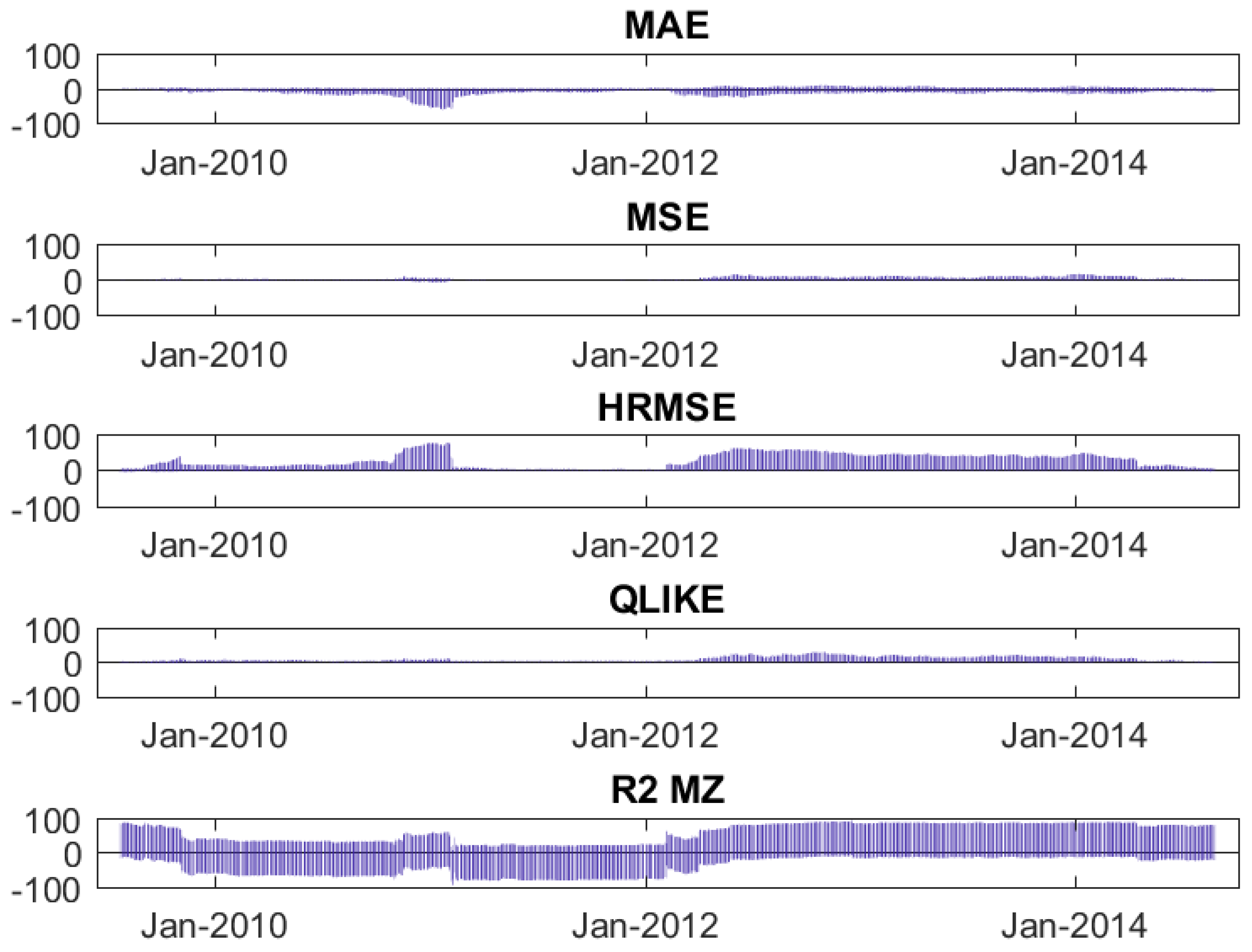
Table 1.
Macro indicators.
| Abbreviation | Complete Name |
|---|---|
| CCONF | Consumer Confidence |
| CPI | Consumer Price Index |
| FOMC | FOMC Rate Decisions |
| GDP | Gross Domestic Product |
| INDPROD | Industrial Production |
| BOP | Balance of Payments |
| JOBLESS | Jobless Claims |
| NFP | Non-Farm Payrolls |
| PPI | Producer Price Index |
| RSALES | Retail Sales |
Table 2.
Selected topics by provider.
| StreetAccount | Thomson Reuters |
|---|---|
| all | all |
| earnings related | earnings pre-announcements |
| M&A | M&A |
| litigation | litigation |
| regulatory | regulatory/company investigation |
| newspapers | financial |
| up/downgrades |
Table 3.
Summary statistics of news stories from the two providers.
| Measure | Min | Quant 5% | Median | Quant 95% | Max | Mean | Std Dev |
|---|---|---|---|---|---|---|---|
| StreetAcc. n. news stories per day | 0.00 | 0.00 | 0.00 | 1.00 | 7.00 | 0.23 | 0.60 |
| T. Reuters n. news stories per day | 0.00 | 0.00 | 0.00 | 1.00 | 3.00 | 0.10 | 0.33 |
| StreetAcc. n. words per day | 0.00 | 0.00 | 0.00 | 102.00 | 1079.00 | 18.18 | 66.68 |
| T. Reuters n. words per day | 0.00 | 0.00 | 0.00 | 68.90 | 390.00 | 8.23 | 31.80 |
Notes: Summary statistics of Street Account news stories topic all and Thomson Reuters news stories topic all, importance low.
Table 4.
Coincident/Total Ratio, percentage of StreetAccount news days, percentage of Thomson Reuters news days.
Table 4.
Coincident/Total Ratio, percentage of StreetAccount news days, percentage of Thomson Reuters news days.
| Topic | Coincident/Total Ratio | % SA News Days | % TR News Days |
|---|---|---|---|
| all | 26.27 | 19.95 | 13.14 |
| earnings | 34.72 | 3.55 | 1.46 |
| litigation | 13.38 | 0.86 | 0.84 |
| M&A | 22.83 | 2.25 | 1.65 |
| regulatory | 3.90 | 1.27 | 0.28 |
Table 5.
Measures transformations.
| Transformation | Formula |
|---|---|
| original measure | x |
| flag if 0 | |
| flag if | |
| flag if | |
| signed square root(x) | |
| signed log(x) | |
| signed square(x) |
Table 6.
Daily news stories measures.
| Variable | N. Transf. |
|---|---|
| STANDARD | |
| n. news stories | 5 |
| n. words | 4 |
| sentiment | 3 |
| ABNORMAL QUANTITY | |
| n. news stories ≥ 2 | 1 |
| UNCERTAINTY | |
| pos and neg news in same day | 1 |
| NEWS BURST INDEX | |
| news burst index (n. news) × | 6 |
| news burst index (n. words) × | 6 |
| SENTIMENT COND. ON QUANTITY | |
| pos sent & n. news stories ≥ 2 | 1 |
| neg sent & n. news stories ≥ 2 | 1 |
| total for each topic | 28 |
| grand total (28 × 31e) | 868 |
Notes: The first column shows the variables grouped by the concepts that originated them. The second column shows the number of transformations, with the total number of measures obtained at the end of the column. We obtain 868 measures. : When the original measure can only be positive, such as number of news stories, the two transformations flag if x > 0 and flag if x < 0 are omitted, leaving five transformations. flag for number of words ≠ 0 is omitted because this measure corresponds to flag for number of news stories ≠ 0. : The transformations applied for are original measure, flag if x > 0, and flag if x < 0. : When the number of transformations equals 1, the measure consists of a flag (1 for the occurrence of the event, and 0 otherwise). : For news burst index we report in the second column the number of combinations of the parameters M and k, and do not apply transformations. e: There are seven topics for StreetAccount news stories and six topics and four levels of importance for Thomson Reuters news stories. 31 stands for the sum of the number of topics of StreetAccount (7) and the number of topics times four levels of importance of Thomson Reuters (24).
Table 7.
Overnight news stories measures.
| Variable | N. Transf. |
|---|---|
| STANDARD | |
| n. news stories | 5 |
| n. words | 4 |
| sentiment | 3 |
| ABNORMAL QUANTITY | |
| n. news stories ≥ 2 | 1 |
| UNCERTAINTY | |
| pos and neg news in same day | 1 |
| SENTIMENT COND. ON QUANTITY | |
| pos sent & n. news stories ≥ 2 | 1 |
| neg sent & n. news stories ≥ 2 | 1 |
| total for each topic | 16 |
| grand total (16 × 31) | 496 |
Table 8.
Weekly news stories measures.
| Variable | N. Transf. |
|---|---|
| STANDARD | |
| av. n. news stories | 5 |
| av. n. words | 4 |
| sentiment | 3 |
| ABNORMAL QUANTITY | |
| av. n. news stories ≥ 1 | 1 |
| NEWS BURST INDEX | |
| news burst index (n. news) × | 2 |
| news burst index (n. words) × | 2 |
| SENTIMENT CONDITIONAL ON QUANTITY | |
| pos sent & av. n. news stories ≥ 1 | 1 |
| neg sent & av. n. news stories ≥ 1 | 1 |
| total for each topic | 19 |
| grand total (19 × 31) | 589 |
a: Quantities result from averaged daily quantities over the last five trading days. Av. refers to average. b: Sentiment results from the sign of the averaged sentiment over the last five trading days.
Table 9.
Monthly news stories measures.
| Variable | N. Transf. |
|---|---|
| STANDARD | |
| av. n. news stories | 5 |
| av. n. words | 4 |
| sentiment | 3 |
| ABNORMAL QUANTITY | |
| av. n. news stories ≥ 1 | 1 |
| NEWS BURST INDEX | |
| news burst index (n. news) x | 2 |
| news burst index (n. words) x | 2 |
| SENTIMENT CONDITIONAL ON QUANTITY | |
| pos sent & av. n. news stories ≥ 1 | 1 |
| neg sent & av. n. news stories ≥ 1 | 1 |
| total for each topic | 19 |
| grand total (19 x 31) | 589 |
Table 10.
Multi-period news stories measures 1/2.
| Variable | N. Transf. |
|---|---|
| QUANTITY VARIATION | |
| day-to-day n. news stories | 7 |
| week-to-day n. news stories | 7 |
| month-to-day n. news stories | 7 |
| day-to-day n. words | 7 |
| week-to-day n. words | 7 |
| month-to-day n. words | 7 |
| NEWS PERSISTENCE/INTERACTION | |
| n. news stories today ≥ 2 & n. news stories day before ≥ 2 | 1 |
| n. news stories today ≥ 2 & av. n. news stories week before ≥ 1 | 1 |
| n. news stories today ≥ 2 & av. n. news stories month before ≥ 1 | 1 |
| SENTIMENT INVERSION | |
| day-to-day sent inv | 1 |
| day-to-day sent inv, neg to pos | 1 |
| day-to-day sent inv, pos to neg | 1 |
| week-to-day sent inv | 1 |
| week-to-day sent inv, neg to pos | 1 |
| week-to-day sent inv, pos to neg | 1 |
| month-to-day sent inv | 1 |
| month-to-day sent inv, neg to pos | 1 |
| month-to-day sent inv, pos to neg | 1 |
Notes: Measures created from the aggregation or comparison of information across different periods, which can differ from one another. : day-to-day Δ n. news stories is equal to the number of news stories on day t minus the number of news stories on day t-1; week-to-day Δ n. news stories and month-to-day Δ n. news stories are equal to the number of news stories on day t minus the average number of news stories in the week before (from t-5 to t-1) and in the month before (from t-22 to t-1), respectively. : news persistence/interaction describes the event in which the amount of news is above a certain threshold in each of two consecutive periods. : day-to-day sent inv describes the event in which sentiment on day t is the opposite of sentiment on day t-1; day-to-day sent inv, neg to pos and day-to-day sent inv, pos to neg describe events in which sentiment is negative on day t-1 and positive on day t and the reverse, respectively.
Table 11.
Multi-period news stories measures 2/2.
| Variable | N. Transf. |
|---|---|
| QUANTITY VARIATION COND. ON SENTIMENT | |
| day-to-day n. news stories > 0 & pos sent today | 1 |
| day-to-day n. news stories > 0 & neg sent today | 1 |
| day-to-day n. news stories < 0 & pos sent day before | 1 |
| day-to-day n. news stories < 0 & neg sent day before | 1 |
| week-to-day n. news stories > 0 & pos sent today | 1 |
| week-to-day n. news stories > 0 & neg sent today | 1 |
| week-to-day n. news stories < 0 & pos sent week before | 1 |
| week-to-day n. news stories < 0 & neg sent week before | 1 |
| month-to-day n. news stories > 0 & pos sent today | 1 |
| month-to-day n. news stories > 0 & neg sent today | 1 |
| month-to-day n. news stories < 0 & pos sent month before | 1 |
| month-to-day n. news stories < 0 & neg sent month before | 1 |
| SENTIMENT COND. ON PAST QUANTITY | |
| pos sent today & n. news stories day before ≥ 2 | 1 |
| neg sent today & n. news stories day before ≥ 2 | 1 |
| pos sent today & av. n. news stories week before ≥ 1 | 1 |
| neg sent today & av. n. news stories week before ≥ 1 | 1 |
| pos sent today & av. n. news stories month before ≥ 1 | 1 |
| neg sent today & av. n. news stories month before ≥ 1 | 1 |
| total for each topic | 72 |
| grand total (72 x 31) | 2232 |
: day-to-day Δ n. news stories & pos sent today describes the event in which the number of news stories on day t is greater than the number of news stories on day t-1 and the sentiment on day t is positive; the remaining variables in the group quantity variation conditional on sentiment are straightforward. The sentiment conditioning the occurrence of the event is that of the period with a greater amount of news; therefore, we look at the sentiment of the period before day t for negative variations. : The variables that belong to the group sentiment conditional on past quantity describe the events in which the sentiment on day t is positive or negative and when, in the period before, the quantity of news is above a threshold that equals 2 for the number of news stories on the day before and 1 for the average number of news stories in the week and the month before.
Table 12.
EPS measures.
| Variable | N. Transf. |
|---|---|
| daily SUE | 8 |
| overnight SUE | 8 |
| weekly SUE | 8 |
| monthly SUE | 8 |
| grand total | 32 |
Notes: EPS measures result from the EPS released in the corresponding period. For example, weekly SUE is equal to the SUE if there was an EPS release in the last week. : In addition to the seven transformations of Table 5, we add a flag variable for the occurrence of an EPS release (1 for occurrence, and 0 otherwise).
Table 13.
Macro-measures.
| Variable | N. Transf. |
|---|---|
| daily Std_CCONF | 8 |
| daily Std_CPI | 8 |
| daily Std_FOMC | 8 |
| daily Std_GDP | 8 |
| daily Std_INDPROD | 8 |
| daily Std_BOP | 8 |
| daily Std_JOB | 8 |
| daily Std_NFP | 8 |
| daily Std_PPI | 8 |
| daily Std_RSALES | 8 |
| overnight Std_Macro | 8 × 10 |
| weekly Std_Macro | 8 × 10 |
| monthly Std_Macro | 8 × 10 |
| grand total | 320 |
Notes: Macro-measures result from the macro-announcement released in the corresponding period, as for EPS measures. : In addition to the seven transformations of Table 5, we add a flag variable for the occurrence of a macro-release (1 for occurrence, and 0 otherwise), as for EPS measures. : Std_Macro refers to the standardized surprise of any of the macro-indicators, which are reported only in the daily group for reasons of brevity. In the second column, the number of transformations is multiplied by the number of macro-indicators.
Table 14.
Google Trends measures.
| Variable | N. Transf. |
|---|---|
| daily GSI | 4 |
| weekly av. GSI | 4 |
| monthly av. GSI | 4 |
| day-to-day GSI | 7 |
| week-to-day GSI | 7 |
| month-to-day GSI | 7 |
| grand total | 33 |
Notes: weekly av. GSI and monthly av. GSI correspond to the average of daily GSI over the last five and twenty-two trading days, respectively. day-to-day Δ GSI is equal to GSI on day t minus GSI on day t-1; week-to-day Δ GSI and month-to-day Δ GSI are equal to GSI on day t minus the average GSI in the week before (from t-5 to t-1) and in the month before (from t-22 to t-1), respectively. : We use four transformations: original measure, signed square root, signed log, and signed square.
Table 15.
Most selected regressors in the LHAR-CJN model. Sample: 2005–2015.
| Past Volatility Components and Leverage | % Selected | % Pos | % Neg | ||||||
|---|---|---|---|---|---|---|---|---|---|
| log | 100.00 | 100.00 | 0.00 | ||||||
| log | 100.00 | 100.00 | 0.00 | ||||||
| log | 100.00 | 100.00 | 0.00 | ||||||
| log | 0.00 | 0.00 | 0.00 | ||||||
| log | 0.00 | 0.00 | 0.00 | ||||||
| log | 3.37 | 3.37 | 0.00 | ||||||
| 91.01 | 0.00 | 91.01 | |||||||
| 70.79 | 0.00 | 70.79 | |||||||
| 33.71 | 0.00 | 33.71 | |||||||
| Macro | Firm-Specific | News | Importance | Topic | Time Aggregation | Measure | % Selected | % Pos | % Neg |
| X | EPS | day | flag for announcement | 58.43 | 58.43 | 0.00 | |||
| X | SA news | earnings | flow: day-to-day | flag if n. words | 28.09 | 28.09 | 0.00 | ||
| X | SA news | all | day | n. news stories | 24.72 | 24.72 | 0.00 | ||
| X | TR news | low | earnings | flow: day-to-day | flag if n. news stories | 23.60 | 23.60 | 0.00 | |
| X | NFP | month | surp | 22.47 | 0.00 | 22.47 | |||
| X | SA news | earnings | flow: day-to-day | flag if n. news stories | 20.22 | 20.22 | 0.00 | ||
| X | TR news | low | earnings | flow: day-to-day | flag if n. news stories | 17.98 | 17.98 | 0.00 | |
| X | TR news | low | earnings | flow: day-to-day | flag if n. words | 16.85 | 16.85 | 0.00 | |
| X | SA news | earnings | flow: day-to-day | flag if n. words | 15.73 | 15.73 | 0.00 | ||
| X | SA news | earnings | day | sqrt n. words | 15.73 | 15.73 | 0.00 | ||
| X | SA news | earnings | day | flag if n. news stories | 14.61 | 14.61 | 0.00 | ||
| X | EPS | day | flag if surp | 13.48 | 13.48 | 0.00 | |||
| X | SA news | earnings | flow: day-to-day | flag if n. news stories | 13.48 | 13.48 | 0.00 | ||
| X | SA news | earnings | day | n. news stories | 12.36 | 12.36 | 0.00 | ||
| X | TR news | medium | earnings | flow: day-to-day | flag if n. news stories | 11.24 | 11.24 | 0.00 | |
| X | SA news | earnings | day | log n. news stories | 11.24 | 11.24 | 0.00 | ||
| X | SA news | earnings | day | sqrt n. news stories | 11.24 | 11.24 | 0.00 | ||
| X | SA news | earnings | day | flag if n. news stories | 11.24 | 11.24 | 0.00 | ||
| X | TR news | medium | earnings | flow: day-to-day | flag if n. words | 10.11 | 10.11 | 0.00 | |
| Google Trends | week | log GSI | 8.99 | 8.99 | 0.00 | ||||
| X | TR news | high | earnings | flow: day-to-day | flag if n. news stories | 8.99 | 8.99 | 0.00 | |
| X | TR news | medium | earnings | flow: day-to-day | flag if n. words | 8.99 | 8.99 | 0.00 | |
| X | TR news | medium | earnings | flow: day-to-day | flag if n. news stories | 8.99 | 8.99 | 0.00 | |
| X | TR news | low | earnings | flow: day-to-day | flag if n. words | 8.99 | 8.99 | 0.00 | |
| X | SA news | all | flow: day-to-day | flag if n. words | 8.99 | 8.99 | 0.00 | ||
| X | TR news | high | earnings | flow: day-to-day | flag if n. news stories | 7.87 | 7.87 | 0.00 | |
| X | TR news | low | earnings | day | log n. words | 7.87 | 7.87 | 0.00 | |
| X | NFP | month | log surp | 6.74 | 0.00 | 6.74 | |||
| X | TR news | low | all | flow: day-to-day | flag if n. words | 6.74 | 6.74 | 0.00 | |
| X | SA news | up/downgrades | flow: day-to-day | flag if n. words | 6.74 | 6.74 | 0.00 | ||
Notes: Ranking of regressors (past volatility components plus the thirty most frequently selected news measures) by percentage of stocks for which they are selected by LASSO in the LHAR-CJN model, percentage of positive and percentage of negative coefficients. Sample: Feburary 2005–February 2015.
Table 16.
Estimated , , , , , , , , , and for the LHAR-CJ and the LHAR-CJN models.
| (a) 2005–2015 | (b) 2005–2007 | |||||
| LHAR-CJ | LHAR-CJN | LHAR-CJ | LHAR-CJN | |||
| () | () | 0.01 | () | () | 0.00 | |
| 0.31 (11.31) | 0.29 (10.77) | 0.25 (5.24) | 0.23 (5.11) | |||
| 0.30 (7.22) | 0.29 (7.24) | 0.30 (3.80) | 0.28 (3.64) | |||
| 0.28 (8.00) | 0.29 (8.12) | 0.01 | 0.21 (2.77) | 0.21 (2.88) | 0.00 | |
| 0.14 (1.91) | 0.12 (1.68) | 0.11 (0.85) | 0.10 (0.81) | |||
| (−0.25) | () | 0.00 | 0.02 (0.27) | 0.02 (0.28) | 0.00 | |
| 0.01 (0.57) | 0.01 (0.57) | 0.00 | 0.01 (0.22) | 0.01 (0.19) | 0.00 | |
| () | () | 0.00 | () | () | 0.00 | |
| (−2.29 ) | () | () | () | 0.00 | ||
| 0.09 () | 0.09 () | 0.00 | () | () | ||
| R | 0.69 | 0.71 | 0.39 | 0.43 | ||
| F-test % rejection hyp. news not significant (sign. level = 5 %) | 97.75% | 64.04% | ||||
| (c) 2007–2009 | (d) 2009–2015 | |||||
| LHAR-CJ | LHAR-CJN | LHAR-CJ | LHAR-CJN | |||
| 0.15 | 0.18 | 0.03 | 0.00 | |||
| (1.90) | (2.18) | () | () | |||
| 0.36 | 0.36 | 0.00 | 0.30 | 0.27 | ||
| (5.71) | (5.62) | (8.23) | (7.71) | |||
| 0.32 | 0.31 | 0.27 | 0.26 | |||
| (3.57) | (3.51) | (4.86) | (4.93) | |||
| 0.15 | 0.15 | 0.00 | 0.27 | 0.28 | 0.01 | |
| (1.92) | (1.88) | (5.55) | (5.61) | |||
| 0.14 | 0.13 | −0.01 | 0.22 | 0.19 | ||
| (1.23) | (1.17) | (1.81) | (1.69) | |||
| 0.00 | 0.00 | |||||
| () | () | () | () | |||
| 0.00 | 0.00 | 0.00 | 0.02 | 0.02 | 0.00 | |
| () | () | (0.50) | (0.52) | |||
| 0.00 | 0.00 | |||||
| () | () | () | () | |||
| 0.00 | ||||||
| () | () | (-2.05) | (-2.29) | |||
| 0.00 | ||||||
| () | () | () | () | |||
| R | 0.70 | 0.71 | 0.53 | 0.58 | ||
| F-test % rejection hyp. news not significant (sign. level = 5 %) | 20.22% | 98.88% | ||||
Notes: Estimated (cross-sectional average) β0, βCd, βCw, βCm, βJd, βJw, βJm, βrd, βrw, and βrm (t-statistics are in brackets), R2 for the LHAR-CJ and the LHAR-CJN models, variation of the coefficients between the two models, and percentage of assets for which the F-test is rejected (null hypothesis: the coefficients of the news variables selected by LASSO are jointly not significant). OLS regression with HAC standard errors, using as explanatory variables for the LHAR-CJN model the regressors of the LHAR-CJ model plus the news variables selected by LASSO. Samples: (a) February 2005–February 2015 (whole sample); (b) February 2005–December 2007 (expansion); (c) December 2007–Junuary 2009 (contraction); (d) June 2009–February 2015 (expansion).
Table 17.
One-step-ahead prediction accuracy of LHAR-CJ and LHAR-CJN models.
| LHAR-CJ | LHAR-CJN | |
|---|---|---|
| MAE | 0.99 (8.99%) | 0.97 (1.12%) |
| MSE | 65.73 (3.37%) | 37.11 (0.00%) |
| HRMSE | 0.90 (0.00%) | 0.83 (48.31%) |
| QLIKE | 1.45 (1.12%) | 1.44 (32.58%) |
| R MZ | 0.49 (25.84%) | 0.51 (74.16%) |
Notes: One-step-ahead MAE, MSE, HRMSE, QLIKE, and R MZ of the LHAR-CJ and the LHAR-CJN models (cross-sectional average). In brackets, for each model and for each metric except R MZ: percentage of assets for which the Diebold-Mariano test rejects with a 5% level the null hypothesis of equal predictive accuracy in favor of that model (p-values are corrected with the Holm–Bonferroni method to control the familywise error rate in the multiple testing framework); for R MZ: percentage of assets for which the metric is higher for that model.
© 2017 by the authors. Licensee MDPI, Basel, Switzerland. This article is an open access article distributed under the terms and conditions of the Creative Commons Attribution (CC BY) license (http://creativecommons.org/licenses/by/4.0/).
Share and Cite
MDPI and ACS Style
Caporin, M.; Poli, F. Building News Measures from Textual Data and an Application to Volatility Forecasting. Econometrics 2017, 5, 35. https://doi.org/10.3390/econometrics5030035
AMA Style
Caporin M, Poli F. Building News Measures from Textual Data and an Application to Volatility Forecasting. Econometrics. 2017; 5(3):35. https://doi.org/10.3390/econometrics5030035
Chicago/Turabian StyleCaporin, Massimiliano, and Francesco Poli. 2017. "Building News Measures from Textual Data and an Application to Volatility Forecasting" Econometrics 5, no. 3: 35. https://doi.org/10.3390/econometrics5030035
Note that from the first issue of 2016, this journal uses article numbers instead of page numbers. See further details here.