HAR Testing for Spurious Regression in Trend

Abstract

The usual t test, the t test based on heteroskedasticity and autocorrelation consistent (HAC) covariance matrix estimators, and the heteroskedasticity and autocorrelation robust (HAR) test are three statistics that are widely used in applied econometric work. The use of these significance tests in trend regression is of particular interest given the potential for spurious relationships in trend formulations. Following a longstanding tradition in the spurious regression literature, this paper investigates the asymptotic and finite sample properties of these test statistics in several spurious regression contexts, including regression of stochastic trends on time polynomials and regressions among independent random walks. Concordant with existing theory (Phillips 1986, 1998; Sun 2004, 2014b) the usual t test and HAC standardized test fail to control size as the sample size $n\to \infty$ in these spurious formulations, whereas HAR tests converge to well-defined limit distributions in each case and therefore have the capacity to be consistent and control size. However, it is shown that when the number of trend regressors $K\to \infty ,$ all three statistics, including the HAR test, diverge and fail to control size as $n\to \infty$. These findings are relevant to high-dimensional nonstationary time series regressions where machine learning methods may be employed.

It is meaningless to talk about ‘confirming’ theories when spurious results are so easily obtained.

(Hendry 1980)

1. Introduction

In a well-cited contribution that emphasized the importance of diagnostic testing in econometrics, (Hendry 1980) highlighted how easy it is to mistake spurious relationships as genuine when using trending data of the type that are so commonly encountered in econometric work, especially in macroeconomics. Spurious regressions occur when conventional significance tests are so seriously biased towards rejection of the null hypothesis of no relationship that the alternative of a genuine relationship is accepted when the variables have no meaningful relationship and may even be statistically independent. Hendry’s article showcased the potential for nonsense regressions with the illustration of a regression between UK consumer prices and cumulative rainfall that displayed a high level of ‘significance’ and passed many—but not all—diagnostic tests.

Spurious regressions continue to attract considerable attention in econometric work, long after the exploratory study by (Yule 1926), the simulation experiments of (Granger and Newbold 1974), and the cautionary warnings made by David Hendry and many other writers since then. The limit theory of (Durlauf and Phillips 1988; Phillips 1986) provided the first analytic steps forward on this subject by explaining the phenomena of persistent null hypothesis rejections in spurious regressions. These two studies helped applied researchers understand the failure of conventional significance tests by showing that in regressions with independent or even correlated trending I(1) data the usual regression t- and F-ratio test statistics do not possess limiting distributions but actually diverge as the sample size $n\uparrow \infty ,$ leading inevitably to rejections of the null of no association. Closely related work by (Phillips and Durlauf 1986; Durlauf and Phillips 1988; Park and Phillips 1988, 1989; Phillips and Hansen 1990; Phillips and Loretan 1991; Phillips 1991) extended the analytics to cover models of cointegrated and reduced rank error correction systems. Much of this work was reviewed in a useful form for practitioners by (Banerjee et al. 1993).

The original study by (Phillips 1986) on spurious regression asymptotics formed the basis of a large subsequent literature that has analyzed spurious regressions among various classes of trend stationary, long memory, nonstationary, and near-nonstationary time series. A recent article by (Ernst et al. 2017) provided further analysis by deriving an expression for the standard deviation of the sample correlation coefficient between two independent standard Brownian motions. While this expression does not explain the phenomenon of spurious regression between two independent random walks, it does reveal that the limiting correlation is not centered on the origin and is highly dispersed. This result complements the original findings in (Phillips 1986) and many subsequent papers that the coefficient of determination in a spurious regression has a well-defined limit distribution and does not converge in probability to zero.

In later work, (Phillips 1998) pointed out that spurious regressions typically reflect the fact that trending data may always be ‘explained’ by a coordinate system of other trending variables—which includes the example of UK price series being well-explained by cumulative rainfall that was used by David Hendry (Hendry 1980). In this broad sense of interpretation, there are no spurious regressions for trending time series, just alternative ‘valid’ representations of the time series trajectories (and those of its limiting stochastic process, given a suitable normalization) in terms of other stochastic processes and deterministic functions of time.

The asymptotic theory in (Phillips 1998) utilized the general representation of a stochastic process in terms of an orthonormal system and provided an extension of the Weierstrass theorem to include the approximation of continuous functions and stochastic processes by Wiener processes. That theory was applied to two classic examples of spurious regressions: regression of stochastic trends on time polynomials, and regressions among independent random walks. Such regressions were shown to reproduce asymptotically in part (and in whole as the regressor space expanded with sample size) the underlying valid representations of one trending process in terms of others, a coordinate system that is entirely analogous to orthonormal or Fourier series representations of a continuous function in terms of polynomials or other simple classes of functions over some interval. An important feature of these ‘valid’ trend relationships is that the coefficients in the representations, like those in the Karhunen–Loève representation of a general stochastic process, are themselves random variables. Randomness in the representation of time-series trajectories is embodied in these coefficients. Much subsequent work has utilized these ideas and analytic methods, either in justifying certain regression representations or in using partial versions of these regression representations to focus on certain features—such as long run features—of the data (notably: Phillips 2005, 2014; Müller 2007; Sun 2004, 2014a, 2014b, 2014c; Hwang and Sun 2018; Müller and Watson 2016, 2018).

An important element in the Hendry (Hendry 1980) discussion of econometric practice was its emphasis on the value of diagnostic testing to ascertain limitations of regressions used in applications. In any empirical regression equation, the properties of the residuals depend inevitably on the properties of the data. To build upon a saying of the famous statistician John Tukey, in the regression equation $y=X\beta +u$ the empirical investigator chooses the variables y and X (possibly with the aid of an autometric regression or a machine learning algorithm) and god gives back $u.$ Any misspecification in the relationship between y and X must therefore be manifest in the properties of $u.$ This is precisely what occurs in a spurious regression—the residual embodies the consequences of a model’s fundamental error of specification—as is revealed by the fact that tests for residual serial correlation such as the Durbin Watson statistic converge in probability to zero in such regressions (Phillips 1986).

Accommodating departures in fitted relationships from conventional assumptions on the properties of regression errors and thereby some of the effects of misspecification has been a longstanding goal of econometrics. One of the great advances in econometric research over the last half-century in response to this goal has been the development of methods of inference that are robust to some of the properties of the data and, particularly, those of the regression error. Such robustness can offer protection against specification error in validating inference. This research has led to the progressive development of heteroskedastic and autocorrelation consistent (HAC) procedures1 and subsequently to heteroskedastic and autocorrelation robust (HAR) methods2 These methods control for the effects of serial dependence and heterogeneity in regression errors and they play a key role in achieving robustness in inference. One area where methods of achieving valid statistical inference via HAC procedures has proved especially important in practice are regressions that involve trending variables and cointegration. This goal motivated the early research on optimal semiparametric approaches to the estimation of cointegrating relationships (Phillips and Hansen 1990) and continues to play a role in subsequent developments in this field (Phillips 2014; Hwang and Sun 2018).

HAC methods generally have good asymptotic properties but they are susceptible to large size distortions in practical work. Several alternative methods have been proposed in the recent literature to improve finite sample performance. Among these, the ‘fixed-b’ lag truncation rule (Kiefer and Vogelsang 2002a, 2002b, 2005) has attracted considerable interest. The method uses a truncation lag M for including sample serial covariances that is proportional to the sample size n (i.e., $M\sim bn$ for some fixed $b\in (0,1$)) and sacrifices consistent variance matrix (and hence standard error) estimation in the interest of achieving improved performance in statistical testing by mirroring finite sample characteristics of test statistics in the new asymptotic theory of these tests. The formation of t ratio and Wald statistics based on HAC estimators without truncation belongs to the more general class of HAR test statistics. There are known analytic advantages to the fixed b approach, primarily related to controlling size distortion. In particular, research by (Jansson 2004; Sun et al. 2011; Sun 2014b) has shown evidence from Edgeworth expansions of enhanced higher-order asymptotic size control in the use of these tests. Recently, (Lazarus et al. 2018; Müller 2014; Sun 2018) have surveyed work in this literature and given recommendations for practical implementation.

In studying spurious regression on trend phenomena, (Phillips 1996, 1998) showed that the use of HAC methods attenuated the misleading divergence rate (under the null hypothesis of no association) by the extent to which the truncation lag $M\to \infty .$ In particular, the divergence rate of the t statistic in a spurious regression involving independent $I\left(1\right)$ variables is $O_p\left(\sqrt{n/M}\right)$ rather than $O_p\left(\sqrt{n}\right)$. Pursuing this philosophy further, (Sun 2004) offered a new solution to deal with inference in spurious regressions. He argued that the divergence of the usual t-statistic arises from the use of a standard error estimator that underestimates the true variation of the ordinary least squares (OLS) estimator. He proposed the use of a fixed-b HAR standard error estimator with a bandwidth proportional to the sample size (where M∼$bn\to \infty$ at the same rate as n). The resulting t-statistic converges to a non-degenerate limiting distribution which depends on nuisance parameters. These discoveries revealed that prudent use of HAR techniques in regression testing might widen the range of inference to include spurious regression.

In the same spirit as (Sun 2004, 2014b), the present contribution analyzes possible advantages in using HAR test statistics in the context of simple trend regressions such as

$$x_t=at+u_t,$$

(1)

where $u_t$ is $I\left(1\right).$ For trend assessment in models of this type it is of interest to test the null hypothesis $H_0:a=0$ of the absence of a deterministic trend in (1). This framework is a prototypical example of much more complex models where deterministic trend, stochastic trends, and trend break components may all be present, hence methods of asymptotically valid estimation and testing are needed. A recent general approach to the consistent estimation of such complex models by machine learning filtering methods is given in (Phillips and Shi 2019).

The present paper considers three types of t test widely used in econometrics: the usual t test, the t test based on HAC covariance matrix estimators, and the fixed-b HAR test. We apply these t-statistics to three classic examples of spurious regressions: regression of stochastic trends on time polynomials, regression of stochastic trends on deterministic time trend and regression among independent random walks. The asymptotic behavior of these three different t-statistics are investigated. In the regression of stochastic trends on time polynomials and the regression among independent random walks, it is shown that the usual t test and HAC based t test are likely to indicate a significant relation with probability that goes to one as the sample size n goes to infinity. However, provided the number of regressors (K) is fixed, the HAR t-statistics converge to well-defined distributions free from nuisance parameters. As a result, when appropriate critical values are drawn from these limiting distributions, the HAR t-statistics would not diverge and valid inference on the regression coefficients would be possible, concordant with (Sun 2004).

In contrast to these results and those of (Sun 2004), we find that HAR t-statistics diverge at rate $\sqrt{K}$ as $K\to \infty$. Hence, the characteristics of spurious regression return even with the use of HAR test statistics in models with an increasing number of regressors. These findings seem relevant for machine learning and autometric model building methods which accommodate large numbers of regressors, including those of the $p>n$ variety where model searching often begins with more regressors than sample observations and penalized methods of estimation are needed to obtain even preliminary results.

Our results also reveal that the other two t-statistics (the usual t and HAC-based t) diverge at greater rates when $K\to \infty$ than when K is fixed. In the regression of stochastic trends on deterministic time trends, we derive the limiting distributions of the statistics under both the null and alternative hypotheses. The HAR test turns out to be the only test which is consistent and has controllable size. All the limit theory for these tests receives strong support in simulations. As will become evident, the appealing asymptotic properties of the HAR test in the fixed number of regressors case are manifest even in situations where some commonly-used regularity conditions in the construction of HAR tests are violated.

The rest of the paper is organized as follows. Section 2 examines regressions of stochastic trends on a complete orthonormal basis in $L_2\left[0,1\right]$ and establishes the limiting distributions of the three different t-statistics with explicit application to the prototypical case of a spurious linear trend regression. Section 3 examines the limit behavior of the t-statistics in regressions among independent random walks. Simulations are reported in Section 4. Section 5 concludes. All proofs are given in the Appendix A, Appendix B and Appendix C.

2. Regression of Stochastic Trend on Time Polynomials

2.1. Model Details and Background

The development in this section concentrates on a simple unit root time series

$$X_t=\sum _{s=1}^{{}_t}{\mu }_s,$$

(2)

whose increments ${\mu }_t$ form a stationary time series with zero mean, finite absolute moments to order $p>2$, and continuous spectral density function $f_{\mu }\left(\lambda \right)$. We assume that $X_t$ satisfies the functional central limit theorem (FCLT)

$$\frac{X_{⌊nr⌋}}{\sqrt{n}}\Rightarrow B\left(r\right)\equiv BM\left({\omega }^2\right),\mathrm{with}{\omega }^2=2\pi f_{\mu }\left(0\right),$$

(3)

for which primitive conditions are well known (e.g., Phillips and Solo 1992). The results that follow are illustrative and apply with suitable modification to more general nonstationary time series, such as near integrated or long memory series, which upon standardization converge to limiting stochastic processes with sample paths that are continuous almost surely.

By the Karhunen–Loève (KL) expansion theorem (e.g., Loève 1963, p. 478) into a countable linear combination of orthogonal functions, the KL representation for the Brownian motion $B\left(r\right)$ is

$$B\left(r\right)=\sum _{k=1}^{\infty }\sqrt{{\lambda }_k}{\phi }_k\left(r\right){\xi }_k=\omega \sqrt{2}\sum _{k=1}^{\infty }\frac{sin\left[\left(k-1/2\right)\pi r\right]}{\left(k-1/2\right)\pi }{\xi }_k,$$

(4)

where

$${\lambda }_k=\frac{4{\omega }^2}{{\left(2k-1\right)}^2{\pi }^2},{\phi }_k\left(r\right)=\sqrt{2}sin\left[\left(k-1/2\right)\pi r\right]$$

are eigenvalues and corresponding eigenfunctions of the Brownian motion covariance kernel ${\omega }^2\left(r\wedge s\right)$, and

$${\xi }_k={\lambda }_k^{-1/2}{\int }_0^{1}B\left(s\right){\phi }_k\left(s\right)ds$$

are independently and identically distributed (iid) as $N\left(0,1\right)$. This series representation of $B\left(r\right)$ is convergent almost surely and uniformly in $r\in \left[0,1\right]$. Denoting $z_k=\sqrt{{\lambda }_k}{\xi }_k$ as the stochastic coefficients, the KL representation (4) could be rewritten as

$$B\left(r\right)=\sum _{k=1}^{\infty }{z}_k{\phi }_k\left(r\right).$$

(5)

Starting from the KL representation of $B\left(r\right)$, (Phillips 1998) studied the asymptotic properties of regressions of $X_t$ on deterministic regressors of the type

$$X_t=\sum _{k=1}^K{\widehat{b}}_k{\phi }_k\left(\frac{t}{n}\right)+{\widehat{u}}_t,$$

(6)

or, equivalently (with ${\widehat{a}}_k={\widehat{b}}_k/\sqrt{n}$),

$$\frac{X_t}{\sqrt{n}}=\sum _{k=1}^K{\widehat{a}}_k{\phi }_k\left(\frac{t}{n}\right)+\frac{{\widehat{u}}_t}{\sqrt{n}}.$$

(7)

Least squares estimation gives

$${\widehat{\alpha }}_K={\left({\widehat{a}}_1,\dots ,{\widehat{a}}_K\right)}^{\prime }={\left({\mathsf{\Phi }}_K^{\prime }{\mathsf{\Phi }}_K\right)}^{-1}{\mathsf{\Phi }}_K^{\prime }X/\sqrt{n},$$

where ${\mathsf{\Phi }}_K={\left({\phi }_{K1},\dots ,{\phi }_{Kn}\right)}^{\prime }$ with ${\phi }_{Kt}={\left({\phi }_1\left(t/n\right),\dots ,{\phi }_K\left(t/n\right)\right)}^{\prime }$, and $X={\left(X_1,\dots ,X_n\right)}^{\prime }$. Let $C_K\in {\mathbb{R}}^K$ be any vector with $C_K^{\prime }{C}_K=1$. When K is fixed and $n\to \infty$, (Phillips 1998) proved that

$$C_K^{\prime }{\widehat{\alpha }}_K\Rightarrow C_K^{\prime }{\int }_0^1{\overline{\phi }}_K\left(r\right)B\left(r\right)dr\equiv N\left(0,C_K^{\prime }{\mathsf{\Lambda }}_K{C}_K\right),$$

where ${\mathsf{\Lambda }}_K=$ diag$\left({\lambda }_1,\dots ,{\lambda }_K\right)$ and ${\overline{\phi }}_K\left(r\right)={\left({\phi }_1\left(r\right),\dots ,{\phi }_K\left(r\right)\right)}^{\prime }$. In the expanding regressors case where $K=K\left(n\right)\to \infty$ and $K/n\to 0$, it was also shown in (Phillips 1998) that

$$C_K^{\prime }{\widehat{\alpha }}_K\Rightarrow N\left(0,{\sigma }_c^2\right)\equiv c^{\prime }Z=\sum _{k=1}^{\infty }{c}_k{z}_k,$$

where $c=\left(c_k\right)\in {\mathbb{R}}^{\infty }$ satisfies $c^{\prime }c=1$, $\mathsf{\Lambda }=$ diag$\left({\lambda }_1,{\lambda }_2,\dots \right)$, ${\sigma }_c^2=c^{\prime }\mathsf{\Lambda }c$, and $Z={\left(z_k\right)}_{k=1}^{\infty }$ are the random coefficients in the KL representation (5). Therefore, the fitted coefficients in regression (7) tend to random variables in the limit as $n\to \infty$ that match those in the KL representation of the limit process $B\left(·\right)$. In other words, least squares regressions reproduce in part (when K is finite) and in whole (when $K\to \infty$) the underlying orthonormal representations.

2.2. Three t-Statistics

Suppose interest centers on testing whether the regression coefficients are significant or more generally whether some linear combination $C_K^{\prime }{\beta }_K$ of the underlying coefficients ${\beta }_K={\left(b_1,\dots ,b_K\right)}^{\prime }$ in the estimated regression (6) is equal to 0, that is

$$H_0:C_K^{\prime }{\beta }_K=0\mathrm{vs}.H_1:C_K^{\prime }{\beta }_K\ne 0.$$

Three types of t-statistics are considered. The first is the usual t-ratio defined as

$$t_{{}_{C_K^{\prime }{\beta }_K}}=\frac{C_K^{\prime }{\widehat{\beta }}_K}{{\left[s_b^2{C}_K^{\prime }{\left({\mathsf{\Phi }}_K^{\prime }{\mathsf{\Phi }}_K\right)}^{-1}{C}_K\right]}^{1/2}}$$

(8)

with $s_b^2=n^{-1}{\sum }_{t=1}^n{\widehat{u}}_t^2=n^{-1}{\sum }_{t=1}^n{\left(X_t-{\widehat{\beta }}_K^{\prime }{\phi }_{Kt}\right)}^2$ the usual error variance estimate. The second t-statistic is constructed by using a HAC variance estimator and has the following representation

$$t_{{}_{C_K^{\prime }{\beta }_K}}^{{}^{HAC}}=\frac{C_K^{\prime }{\widehat{\beta }}_K}{{\widehat{\omega }}_{C_K^{\prime }{\beta }_K}},$$

(9)

where

$${\widehat{\omega }}_{C_K^{\prime }{\beta }_K}^2=C_K^{\prime }{\left({\mathsf{\Phi }}_K^{\prime }{\mathsf{\Phi }}_K\right)}^{-1}\left[n{\widehat{\mathrm{lrvar}}}_{HAC}\left({\widehat{u}}_t{\phi }_{Kt}\right)\right]{\left({\mathsf{\Phi }}_K^{\prime }{\mathsf{\Phi }}_K\right)}^{-1}{C}_K$$

(10)

with

$${\widehat{\mathrm{lrvar}}}_{HAC}\left({\eta }_t\right)=\sum _{j=-M}^{M}k\left(\frac{j}{M}\right)c\left(j,\eta \right)\mathrm{and}c\left(j,\eta \right)=\frac{1}{n}\sum _{1\le t,t+j\le n}{\eta }_t{\eta }_{t+j}^{\prime }.$$

(11)

Here, ${\widehat{\mathrm{lrvar}}}_{HAC}\left({\eta }_t\right)$ is a kernel estimate of the long run variance of its argument, $k\left(·\right)$ is a lag kernel, M is a bandwidth parameter satisfying $M/n+1/M\to 0$ as $n\to \infty ,$ and the argument ${\eta }_t={\widehat{u}}_t{\phi }_{Kt}$ in (10).

If we choose a fixed $b\in (0,1]$ and set $M=⌊bn⌋$, the condition $M/n+1/M\to 0$ as $n\to \infty$ is violated. In that case, the long run variance estimate is a fixed-b estimate and leads to the HAR t-statistic

$$t_{{}_{C_K^{\prime }{\beta }_K}}^{{}^{HAR}}=\frac{C_K^{\prime }{\widehat{\beta }}_K}{{\check{\omega }}_{C_K^{\prime }{\beta }_K}},$$

(12)

where

$${\check{\omega }}_{C_K^{\prime }{\beta }_K}^2=C_K^{\prime }{\left({\mathsf{\Phi }}_K^{\prime }{\mathsf{\Phi }}_K\right)}^{-1}\left[n{\widehat{\mathrm{lrvar}}}_{HAR}\left({\widehat{u}}_t{\phi }_{Kt}\right)\right]{\left({\mathsf{\Phi }}_K^{\prime }{\mathsf{\Phi }}_K\right)}^{-1}{C}_K$$

(13)

with

$${\widehat{\mathrm{lrvar}}}_{HAR}\left({\eta }_t\right)=\sum _{j=-\left(n-1\right)}^{\left(n-1\right)}{k}_b\left(\frac{j}{n}\right)c\left(j,\eta \right),c\left(j,\eta \right)=\frac{1}{n}\sum _{1\le t,t+j\le n}{\eta }_t{\eta }_{t+j}^{\prime },$$

(14)

$k_b\left(\frac{j}{n}\right)=k\left(\frac{j}{nb}\right)$, and $k\left(·\right)$ is a lag kernel function as before.

With minor changes of the proof given in (Phillips 1998), it is easy to deduce that for fixed K, $t_{{}_{C_K^{\prime }{\beta }_K}}\sim O_p\left(\sqrt{n}\right)$ and $t_{{}_{C_K^{\prime }{\beta }_K}}^{{}^{HAC}}\sim O_p\left(\sqrt{n/M}\right)$ as $n\to \infty ,$ as discussed earlier. Therefore, such tests indicate statistically significant regression coefficients with probability that goes to one as $n\to \infty$. These results match what is now standard spurious regression limit theory for inference.

In addition, as we show in Theorem 2 below, the large regressor case where $K\to \infty$ leads to different results. In this case, both t-statistics $t_{{}_{C_K^{\prime }{\beta }_K}}$ and $t_{{}_{C_K^{\prime }{\beta }_K}}^{{}^{HAC}}$ have greater rates of divergence that depend on the expansion rate of $K,$ given by $t_{{}_{C_K^{\prime }{\beta }_K}}=O_p\left(\sqrt{nK}\right)$ and $t_{{}_{C_K^{\prime }{\beta }_K}}^{{}^{HAC}}=O_p\left(\sqrt{nK/M}\right)$. Thus, with the addition of more regressors the combined effect of the regression coefficients—as well as that of the individual coefficients—appears more significant and diverges when $K\to \infty$ as $n\to \infty .$ In consequence, large numbers of regressors effectively worsen the spurious regression problem.

Is there a test which does not always indicate that coefficients ${\widehat{\beta }}_K$ are significant in the ‘spurious’ regression (6)? As the results of (Sun 2004) show, the answer is positive for the case where K is fixed. In this event, the HAR test is appealing in the sense that $t_{{}_{C_K^{\prime }{\beta }_K}}^{{}^{HAR}}\sim O_p\left(1\right)$ when $n\to \infty$ and K is fixed, so that test size is controlled in the limit. Therefore, when appropriate critical values obtained from the limit distribution of $t_{{}_{C_K^{\prime }{\beta }_K}}^{{}^{HAR}}$ are employed, the coefficients ${\widehat{\beta }}_K$ do not inevitably signal significance as $n\to \infty$ and the usual misleading test implications of spurious regression do not manifest. However, in the important case where the regressor space expands and $K\to \infty$, the test statistic $t_{{}^{C_K^{\prime }{\beta }_K}}^{{}^{HAR}}$ diverges to infinity at rate $O_p\left(\sqrt{K}\right)$ and the coefficients ${\widehat{\beta }}_K$ become significant again even under HAR testing.

These results are collected in the following two theorems.

Theorem 1.

For fixed K, as $n\to \infty$ and $M/n+1/M\to 0$, we have

(i)

$$\frac{t_{{}_{C_K^{\prime }{\beta }_K}}}{\sqrt{n}}\Rightarrow \frac{C_K^{\prime }{Z}_K}{{\left[{\int }_0^1{\underline{B}}_{{\phi }_K}^2\right]}^{1/2}};$$

(ii)

$$\sqrt{\frac{M}{n}}{t}_{{}_{C_K^{\prime }{\beta }_K}}^{{}^{HAC}}\Rightarrow \frac{C_K^{\prime }{Z}_K}{{\left\{{\int }_{-1}^{1}k\left(s\right)ds{\int }_0^1{\underline{B}}_{{\phi }_K}^2{\left(C_K^{\prime }{\overline{\phi }}_K\right)}^2\right\}}^{1/2}};$$

(iii)

$$\begin{array}{cc}\hfill t_{{}_{C_K^{\prime }{\beta }_K}}^{{}^{HAR}}& \Rightarrow \frac{C_K^{\prime }{Z}_K}{{\left\{{\int }_0^1{\int }_0^1{k}_b\left(r-q\right){\underline{B}}_{{\phi }_K}\left(r\right){\underline{B}}_{{\phi }_K}\left(q\right)\left[C_K^{\prime }{\overline{\phi }}_K\left(r\right)\right]\left[C_K^{\prime }{\overline{\phi }}_K\left(q\right)\right]drdq\right\}}^{1/2}}\hfill \\ \hfill & \equiv \frac{C_K^{\prime }{Z}_K^W}{{\left\{{\int }_0^1{\int }_0^1{k}_b\left(r-q\right){\underline{W}}_{{\phi }_K}\left(r\right){\underline{W}}_{{\phi }_K}\left(q\right)\left[C_K^{\prime }{\overline{\phi }}_K\left(r\right)\right]\left[C_K^{\prime }{\overline{\phi }}_K\left(q\right)\right]drdq\right\}}^{1/2}},\hfill \end{array}$$

where $Z_K={\left(z_k\right)}_{k=1}^K$ are the random coefficients in orthonormal representation (5), ${\underline{B}}_{{\phi }_K}\left(r\right)=B\left(r\right)-$$Z_K^{\prime }{\overline{\phi }}_K\left(r\right)$, $Z_K^W=Z_K/\omega ={\int }_0^{1}W{\overline{\phi }}_K$, $W\left(·\right)\equiv BM\left(1\right),$${\omega }^2=2\pi f_{\mu }\left(0\right)$, and ${\underline{W}}_{{\phi }_K}\left(r\right)={\underline{B}}_{{\phi }_K}\left(r\right)/\omega =W\left(r\right)-{\left(Z_K^W\right)}^{\prime }{\overline{\phi }}_K\left(r\right)$.

Remark 1.

The fixed-b HAR based t-statistic $t_{{}_{C_K^{\prime }{\beta }_K}}^{{}^{HAR}}$ asymptotically follows a well-defined limit distribution when the number of regressors K is fixed. The limit distribution is free from nuisance parameters and is easily computable but depends on the lag kernel as well as the form of the trend regressors, which influence the detrended standard Brownian motion process ${\underline{W}}_{{\phi }_K}.$ The asymptotic critical values, therefore, differ from those of the usual standard normal limit distribution of a t-statistic. But the specific features of the limit distribution of $t_{{}_{C_K^{\prime }{\beta }_K}}^{{}^{HAR}},$ which retain randomness in the denominator of the limiting statistic, help to control size in finite sample testing.

Theorem 2.

As $n,K\to \infty$, $M/n+1/M\to 0$ and $K^{5/2}/n+K^{3/2}/n^{\frac{1}{2}-\frac{1}{p}}\to 0$, the following results hold:

(i)

$$\frac{t_{{}_{C_K^{\prime }{\beta }_K}}}{\sqrt{nK}}=\frac{C_K^{\prime }{Z}_K}{{\left[K{\int }_0^1{\underline{B}}_{{\phi }_K}^2\right]}^{1/2}}+o_p\left(1\right)=O_p\left(1\right),$$

where $K{\int }_0^1{\underline{B}}_{{\phi }_K}^2={\omega }^2/{\pi }^2+o_p\left(1\right)$.

(ii)

$$\sqrt{\frac{M}{nK}}{t}_{{}_{C_K^{\prime }{\beta }_K}}^{{}^{HAC}}=\frac{C_K^{\prime }{Z}_K}{{\left[K{\int }_{-1}^{1}k\left(s\right)ds{\int }_0^1{\underline{B}}_{{\phi }_K}^2{\left[C_K^{\prime }{\overline{\phi }}_K\right]}^2\right]}^{1/2}}+o_p\left(1\right)=O_p\left(1\right),$$

(iii)

$$\frac{t_{{}_{C_K^{\prime }{\beta }_K}}^{{}^{HAR}}}{\sqrt{K}}=\frac{C_K^{\prime }{Z}_K}{{\left\{K{\int }_0^1{\int }_0^1{k}_b\left(r-q\right){\underline{B}}_{{\phi }_K}\left(r\right){\underline{B}}_{{\phi }_K}\left(q\right)C_K^{\prime }{\overline{\phi }}_K\left(r\right)C_K^{\prime }{\overline{\phi }}_K\left(q\right)drdq\right\}}^{1/2}}+o_p\left(1\right)=O_p\left(1\right).$$

Remark 2.

Theorem 2 shows that all three t-statistics diverge as $n\to \infty$ but at different rates, each of which depends on K. The divergence rate of the fixed-b test statistic $t_{{}_{C_K^{\prime }{\beta }_K}}^{{}^{HAR}}=O_p\left(\sqrt{K}\right)$ is the slowest and depends only on $K.$ These results strengthen the findings in (Phillips 1998) that attempts to deal with serial dependence in controlling size in significance testing generally fail when enough effort is put into the regression design to fit the trajectory. This failure now includes HAR testing when $K\to \infty$. All the tests are therefore ultimately confirmatory of the existence of a ‘relationship’—in the present case a coordinate representation relationship among different types of trends, at least when a complete representation is attempted by allowing the number of regressors K to diverge with $n.$ The results of the theorem may be interpreted to mean that when a serious attempt is made to model a stochastic trend using deterministic functions (either a large number of such regressors or regressors that are carefully chosen to provide a successful representation and trajectory fit) it will end up being successful even when a spurious regression robust method such as fixed-b HAR test is used.

An additional matter concerning the form of these tests may usefully be highlighted. To construct the HAC and HAR t-statistics, the following condition

$$\mathrm{Var}\left(\frac{{\mathsf{\Phi }}_K^{\prime }X}{\sqrt{n}}\right)=\mathrm{Var}\left(\frac{1}{\sqrt{n}}\sum _{t=1}^n{\phi }_{Kt}{X}_t\right)={\mathsf{\Gamma }}_0+\sum _{j=1}^{n-1}\left(1-\frac{j}{n}\right)\left({\mathsf{\Gamma }}_j+{\mathsf{\Gamma }}_j^{\prime }\right)$$

(15)

with ${\mathsf{\Gamma }}_j=E\left({\phi }_{Kt}{X}_t{X}_{t-j}^{\prime }{\phi }_{K\left(t-j\right)}^{\prime }\right)$ is usually imposed (e.g., Kiefer et al. 2000; Kiefer and Vogelsang 2002a, 2002b) as in standard approaches to robust covariance matrix estimation. In other words, the process $\left\{{\phi }_{Kt}{X}_t\right\}$ is typically assumed to be unconditionally stationary or weakly dependent with uniformly bounded second moments so that series such as (15) converge. However, this condition is violated in both regressions (6) and (7) as

$$E\left({\phi }_{Kt}{X}_t{X}_{t-j}^{\prime }{\phi }_{K\left(t-j\right)}^{\prime }\right)={\phi }_{Kt}E\left(\sum _{s=1}^t{\mu }_s\sum _{\tau =1}^{t-j}{\mu }_{\tau }\right){\phi }_{K\left(t-j\right)}^{\prime }$$

depends on t. For example, when the components ${\mu }_s$ are $iid$$\left(0,{\sigma }^2\right)$ with partial sums satisfying (3) then

$$E\left({\phi }_{Kt}{X}_t{X}_{t-j}^{\prime }{\phi }_{K\left(t-j\right)}^{\prime }\right)=\left(t-j\right){\sigma }^2{\phi }_{Kt}{\phi }_{K\left(t-j\right)}^{\prime }$$

depends on t. Regardless of this violation, HAC and HAR t-statistics may still be constructed in the traditional way; and the HAR statistic, $t_{{}_{C_K^{\prime }{\beta }_K}}^{{}^{HAR}}$ has nuisance parameter-free asymptotic properties even though the above unconditional stationarity condition is not satisfied.

The above results apply straightforwardly to the simple case of a spurious linear regression on trend where the time series is a unit root process generated by

$$X_t=at+X_t^0,t=1,\dots ,n,$$

(16)

with $a=0$ and $X_t^0={\sum }_{s=1}^t{\mu }_s$ is the partial sum of a zero mean stationary process $\left\{{\mu }_s\right\}$ with continuous spectral density $f_{\mu }\left(\lambda \right).$ The standardized process $X_n\left(r\right)=n^{-1/2}{X}_{⌊nr⌋}^0$ satisfies the functional law

$$X_n\left(r\right)\Rightarrow B\left(r\right)\equiv BM\left({\omega }^2\right),{\omega }^2=2\pi f_{\mu }\left(0\right)>0.$$

The fitted regression model is

$$X_t=\widehat{a}t+{\widehat{u}}_t,\mathrm{or}\mathrm{equivalently},\frac{X_t}{\sqrt{n}}=\left(\sqrt{n}\widehat{a}\right)\frac{t}{n}+\frac{{\widehat{u}}_t}{\sqrt{n}},$$

(17)

where $\widehat{a}={\sum }_{t=1}^{n}t{X}_t/{\sum }_{t=1}^n{t}^2$ is the LS estimate of $a,$ which satisfies (Durlauf and Phillips 1988)

$$\sqrt{n}\left(\widehat{a}-a\right)=\frac{n^{-5/2}{\sum }_{t=1}^{n}t{X}_t^0}{n^{-3}{\sum }_{t=1}^n{t}^2}\Rightarrow 3{\int }_0^{1}rB\left(r\right)dr\equiv N\left(0,\frac{6}{5}{\omega }^2\right),$$

(18)

so that $\widehat{a}$ is consistent, including the case where $a=0.$ However, as is well known, the usual t-statistic has order $O_p\left(\sqrt{n}\right)$ and diverges as $n\to \infty ,$ indicating a significant relationship between $\left\{X_t\right\}$ and t in spite of the fact that $a=0.$ This outcome follows directly from Theorem 1 and the (alternate) representation for the standard Brownian motion $W\left(r\right)$ as

$$W\left(r\right)=r{\xi }_0+\sqrt{2}\sum _{k=1}^{\infty }\frac{sin\left[k\pi r\right]}{k\pi }{\xi }_k\mathrm{with}{\xi }_k\equiv \mathrm{iid}N\left(0,1\right),$$

(19)

which implies that

$$n^{-1/2}{X}_{⌊nr⌋}^0\Rightarrow B\left(r\right)=\omega ·W\left(r\right)=\left(\omega {\xi }_0\right)r+\left(\omega {\xi }_k\right)\sqrt{2}\sum _{k=1}^{\infty }\frac{sin\left[k\pi r\right]}{k\pi }.$$

Thus, when $a=0$, the scaled LS estimator $\sqrt{n}\widehat{a}$ has a random limit ${\xi }_a\equiv N\left(0,\frac{6}{5}{\omega }^2\right)$ from (18) that approximates but does not exactly reproduce the leading random coefficient term $\left(\omega {\xi }_0\right)$ in the representation (19). Importantly in this case, the deterministic functions in (19) are not orthonormal and there is dependence in $L_2\left[0,1\right]$ between the functions r and ${\left\{\left(\sqrt{2}sin\left[k\pi r\right]\right)/\left(k\pi \right)\right\}}_{k=1}^{\infty }.$ This dependence induces an asymptotic inefficiency in the trend coefficient estimate $\widehat{a}$, since $\frac{6}{5}{\omega }^2>$ Var $\left(\omega {\xi }_0\right)={\omega }^2$.

Next, in testing $H_0:a=0$ versus $H_1:a\ne 0,$ the following statistics are considered:

$$\begin{array}{cc}\hfill t_a& =\frac{\widehat{a}}{s_a}=\frac{\widehat{a}}{{\left\{\left[n^{-1}{\sum }_{t=1}^n{\left({\widehat{u}}_t\right)}^2\right]{\left({\sum }_{t=1}^n{t}^2\right)}^{-1}\right\}}^{1/2}},\hfill \end{array}$$

(20)

$$\begin{array}{cc}\hfill t_a^{{}^{HAC}}& =\frac{\widehat{a}}{{\widehat{\omega }}_a}=\frac{\widehat{a}}{{\left\{{\left({\sum }_{t=1}^n{t}^2\right)}^{-1}\left[n{\widehat{\mathrm{lrvar}}}_{HAC}\left(t{\widehat{u}}_t\right)\right]{\left({\sum }_{t=1}^n{t}^2\right)}^{-1}\right\}}^{1/2}},\hfill \end{array}$$

(21)

$$\begin{array}{cc}\hfill t_a^{{}^{HAR}}& =\frac{\widehat{a}}{{\check{\omega }}_a}=\frac{\widehat{a}}{{\left\{{\left({\sum }_{t=1}^n{t}^2\right)}^{-1}\left[n{\widehat{\mathrm{lrvar}}}_{HAR}\left(t{\widehat{u}}_t\right)\right]{\left({\sum }_{t=1}^n{t}^2\right)}^{-1}\right\}}^{1/2}},\hfill \end{array}$$

(22)

where

$${\widehat{\mathrm{lrvar}}}_{HAC}\left(t{\widehat{u}}_t\right)=\sum _{j=-M}^{M}k\left(\frac{j}{M}\right)\left[\frac{1}{n}\sum _{1\le t,t+j\le M}{\widehat{u}}_t{\widehat{u}}_{t+j}t\left(t+j\right)\right]\mathrm{with}M/n+1/M\to 0\mathrm{as}n\to \infty ,$$

$${\widehat{\mathrm{lrvar}}}_{HAR}\left(t{\widehat{u}}_t\right)=\sum _{j=-\left(n-1\right)}^{\left(n-1\right)}{k}_b\left(\frac{j}{n}\right)\left[\frac{1}{n}\sum _{1\le t,t+j\le M}{\widehat{u}}_t{\widehat{u}}_{t+j}t\left(t+j\right)\right]\mathrm{for}\mathrm{some}\mathrm{fixed}b\in (0,1],$$

$k\left(·\right)$ is a kernel function, $k_b\left(j/n\right)=k\left(j/\left(nb\right)\right)$ and ${\widehat{u}}_t=X_t-\widehat{a}t$ for $t=1,\dots ,n$. The asymptotic properties of these test statistics follow in the same way as before when $n\to \infty$ with $M/n+1/M\to 0,$ giving the following results.

(i) Under $H_0:a=0$,

$$\begin{array}{c}\frac{t_a}{\sqrt{n}}\Rightarrow \frac{\sqrt{3}{\int }_0^{1}rB}{{\left\{{\int }_0^1{\underline{B}}^2\right\}}^{1/2}},\end{array}$$

(23)

$$\begin{array}{c}\sqrt{\frac{M}{n}}{t}_a^{{}^{HAC}}\Rightarrow \frac{{\int }_0^{1}rB}{{\left\{{\int }_{-1}^{1}k\left(s\right)ds{\int }_0^1{r}^2{\underline{B}}^2\right\}}^{1/2}},\end{array}$$

(24)

$$\begin{array}{c}{t}_a^{{}^{HAR}}\Rightarrow \frac{{\int }_0^{1}rB}{{\left\{{\int }_0^1{\int }_0^1{k}_b\left(r-q\right)\underline{B}\left(r\right)\underline{B}\left(q\right)rqdrdq\right\}}^{1/2}}\equiv \frac{{\int }_0^{1}rW}{{\left\{{\int }_0^1{\int }_0^1{k}_b\left(r-q\right)\underline{W}\left(r\right)\underline{W}\left(q\right)rqdrdq\right\}}^{1/2}};\end{array}$$

(25)

(ii) Under $H_1:a\ne 0$,

$$\begin{array}{c}\frac{t_a}{n}\Rightarrow \frac{a}{{\left(3{\int }_0^1{\underline{B}}^2\right)}^{1/2}},\end{array}$$

(26)

$$\begin{array}{c}\frac{\sqrt{M}}{n}{t}_a^{{}^{HAC}}\Rightarrow \frac{a}{{\left[9{\int }_{-1}^{1}k\left(s\right)ds{\int }_0^1{r}^2{\underline{B}}^2\right]}^{1/2}},\end{array}$$

(27)

$$\begin{array}{c}\frac{t_a^{{}^{HAR}}}{\sqrt{n}}\Rightarrow \frac{a}{{\left[9{\int }_0^1{\int }_0^1{k}_b\left(r-q\right)\underline{B}\left(r\right)\underline{B}\left(q\right)rqdrdq\right]}^{1/2}},\end{array}$$

(28)

where $\underline{B}\left(r\right):=B\left(r\right)-3\left({\int }_0^{1}sB\left(s\right)ds\right)r$ and $B\left(r\right)\equiv \omega W\left(r\right)$. Thus, under the null hypothesis both $t_a=O_p\left(\sqrt{n}\right)$ and $t_a^{{}^{HAC}}=O_p\left(\sqrt{n/M}\right)$ diverge but $t_a^{{}^{HAR}}=O_p\left(1\right)$ and has a well defined nuisance parameter free limit distribution that may be used in statistical testing. Under the alternative hypothesis, all the listed statistics are divergent but at different rates. Only $t_a^{{}^{HAR}}$ has effective discriminatory power, being consistent and having controllable size. These results match those in (Sun 2004, 2014a) showing that for simple trend misspecifications like that of a finite degree polynomial trend function in place of a stochastic trend, use of fixed-b HAR testing controls size and leads to a consistent test.

3. Regressions Among Independent Random Walks

This section extends these ideas to regressions among independent random walks. Let $B\left(·\right)$ be a Brownian motion on the interval $\left[0,1\right]$. (Phillips 1998) proved that there exist a sequence of independent standard Brownian motions ${\left\{W_i\right\}}_{i=1}^K$ that are independent of $B\left(·\right)$, and a sequence of variables ${\left\{d_i\right\}}_{i=1}^K$ defined on an augmented probability space $\left(\mathsf{\Omega },\mathcal{F},P\right)$ such that, as $K\to \infty$,

$$B\left(r\right)\sim \sum _{i=1}^{\infty }{d}_i{W}_i\left(r\right)\mathrm{in}{L}_2\left[0,1\right]\mathrm{a}.\mathrm{s}.\left(P\right).$$

(29)

The random coefficients $d_i$ are statistically dependent on $B\left(·\right)$. Replacing the Wiener processes $W_i$ by orthogonal functions $V_i\left(r\right)$ in $L_2\left[0,1\right]$ using the Gram-Schmidt process

$$\begin{array}{cc}\hfill V_1& =W_1,\hfill \\ \hfill V_2& =W_2-\left({\int }_0^1{W}_2{V}_1\right){\left({\int }_0^1{V}_1^2\right)}^{-1}{V}_1,\hfill \\ \hfill V_3& =W_3-\left({\int }_0^1{W}_3{V}_a^{\prime }\right){\left({\int }_0^1{V}_a{V}_a^{\prime }\right)}^{-1}{V}_a,V_a^{\prime }=\left[V_1,V_2\right],\mathrm{etc},\hfill \end{array}$$

gives the representation

$$B\left(r\right)\sim \sum _{i=1}^{\infty }{e}_i{V}_i\left(r\right)\mathrm{with}{e}_i=\left({\int }_0^{1}B{V}_i\right){\left({\int }_0^1{V}_i^2\right)}^{-1}.$$

(30)

In the following, we consider the unit root process $y_t={\sum }_{s=1}^t{\mu }_s$ with mean zero stationary components $\left\{{\mu }_s\right\}$ with continuous spectral density $f_{\mu }\left(\lambda \right)$ and satisfying the functional law

$$n^{-1/2}{y}_{⌊nr⌋}\Rightarrow B\left(r\right)\equiv BM\left({\omega }^2\right),{\omega }^2=2\pi f_{\mu }\left(0\right)>0.$$

Let $x_t=\left(x_{kt}\right)={\left({\sum }_{j=1}^t{\mu }_{kj}\right)}_{k=1}^K$ be K independent standard Gaussian random walks, all of which are independent of $y_t$. Consider the linear regression $y_t={\widehat{b}}_x^{\prime }{x}_t+{\widehat{u}}_t$, based on $n>K$ observations of these series. The large n asymptotic behavior of ${\widehat{b}}_x$ is (Phillips 1986) ${\widehat{b}}_x\Rightarrow {\left({\int }_0^1{W}_x{W}_x^{\prime }\right)}^{-1}\left({\int }_0^1{W}_{x}B\right),$ where $W_x$ is the vector standard Brownian motion weak limit of the standardized partial sum processes $n^{-1/2}{x}_{⌊n·⌋}$.

Suppose we orthogonalize the regressors $\left\{x_{k·}={\left(x_{kt}\right)}_{t=1}^n:k=1,\dots ,K\right\}$ using the Gram-Schmidt process

$$\begin{array}{cc}\hfill z_{1t}& =x_{1t},\hfill \\ \hfill z_{2t}& =x_{2t}-\left(x_{2·}^{\prime }{x}_{1·}\right){\left(x_{1·}^{\prime }{x}_{1·}\right)}^{-1}{x}_{1t},\hfill \\ \hfill z_{3t}& =x_{3t}-\left(x_{3·}^{\prime }{X}_a\right){\left(X_a^{\prime }{X}_a\right)}^{-1}{x}_{at},X_a:=\left[x_{1·},x_{2·}\right]:=\left[x_{a·}^{\prime }\right],\mathrm{etc}.\hfill \end{array}$$

By standard weak convergence arguments we have

$$n^{-1/2}{z}_{1⌊n·⌋}\Rightarrow V_1\left(·\right),n^{-1/2}{z}_{2⌊n·⌋}\Rightarrow V_2\left(·\right),n^{-1/2}{z}_{3⌊n·⌋}\Rightarrow V_3\left(·\right),\mathrm{etc}.$$

Now let $z_t={\left(z_{kt}\right)}_{k=1}^K$, and consider the regression

$$y_t={\widehat{b}}_{zK}^{\prime }{z}_t+{\widehat{u}}_t.$$

(31)

The LS estimator ${\widehat{b}}_{zK}={\left[{\sum }_{t=1}^n{z}_t{z}_t^{\prime }\right]}^{-1}{\sum }_{t=1}^n{z}_t{y}_t$ has the limit

$${\widehat{b}}_{zK}\Rightarrow {\left({\int }_0^1{\overline{V}}_K{\overline{V}}_K^{\prime }\right)}^{-1}\left({\int }_0^1{\overline{V}}_{K}B\right)\equiv E_K:={\left(e_k\right)}_{k=1}^K,$$

where ${\overline{V}}_K={\left(V_k\right)}_{k=1}^K$ is a $K\times 1$ vector. Thus, the empirical regression of $y_t$ on $z_t$ reproduces the first K terms in the representation of the limit Brownian motion B in terms of an orthogonalized coordinate system formed from K independent standard Brownian motions.

Suppose now that we are interested in testing whether a linear combination of $b_{zK}$ equals zero, viz.,

$$H_0:C_K^{\prime }{b}_{zK}=0\mathrm{vs}.H_1:C_K^{\prime }{b}_{zK}\ne 0$$

with $C_K\in {\mathbb{R}}^K$ satisfying $C_K^{\prime }{C}_K=1$. Again, three types of t-statistics are considered:

$$\begin{array}{cc}\hfill t_{b_{zK}}& =\frac{C_K^{\prime }{\widehat{b}}_{zK}}{s_{b_{zK}}}=\frac{C_K^{\prime }{\widehat{b}}_{zK}}{{\left\{C_K^{\prime }\left[n^{-1}{\sum }_{t=1}^n{\left({\widehat{u}}_t\right)}^2\right]{\left({\sum }_{t=1}^n{z}_t{z}_t^{\prime }\right)}^{-1}{C}_K\right\}}^{1/2}},\hfill \end{array}$$

(32)

$$\begin{array}{cc}\hfill t_{b_{zK}}^{{}^{HAC}}& =\frac{C_K^{\prime }{\widehat{b}}_{zK}}{{\widehat{\omega }}_{b_{zK}}}=\frac{C_K^{\prime }{\widehat{b}}_{zK}}{{\left\{C_K^{\prime }{\left({\sum }_{t=1}^n{z}_t{z}_t^{\prime }\right)}^{-1}\left[n{\widehat{\mathrm{lrvar}}}_{HAC}\left(z_t{\widehat{u}}_t\right)\right]{\left({\sum }_{t=1}^n{z}_t{z}_t^{\prime }\right)}^{-1}{C}_K\right\}}^{1/2}},\hfill \end{array}$$

(33)

$$\begin{array}{cc}\hfill t_{b_{zK}}^{{}^{HAR}}& =\frac{C_K^{\prime }{\widehat{b}}_{zK}}{{\check{\omega }}_{b_{zK}}}=\frac{C_K^{\prime }{\widehat{b}}_{zK}}{{\left\{C_K^{\prime }{\left({\sum }_{t=1}^n{z}_t{z}_t^{\prime }\right)}^{-1}\left[n{\widehat{\mathrm{lrvar}}}_{HAR}\left(z_t{\widehat{u}}_t\right)\right]{\left({\sum }_{t=1}^n{z}_t{z}_t^{\prime }\right)}^{-1}{C}_K\right\}}^{1/2}},\hfill \end{array}$$

(34)

where

$${\widehat{\mathrm{lrvar}}}_{HAC}\left(z_t{\widehat{u}}_t\right)=\sum _{j=-M}^{M}k\left(\frac{j}{M}\right)\left[\frac{1}{n}\sum _{1\le t,t+j\le M}{z}_t{\widehat{u}}_t{\widehat{u}}_{t+j}{z}_{t+j}^{\prime }\right]\mathrm{with}M/n+1/M\to 0\mathrm{as}n\to \infty ,$$

$${\widehat{\mathrm{lrvar}}}_{HAR}\left(z_t{\widehat{u}}_t\right)=\sum _{j=-\left(n-1\right)}^{\left(n-1\right)}{k}_b\left(\frac{j}{n}\right)\left[\frac{1}{n}\sum _{1\le t,t+j\le M}{z}_t{\widehat{u}}_t{\widehat{u}}_{t+j}{z}_{t+j}^{\prime }\right]\mathrm{for}\mathrm{some}\mathrm{fixed}b\in (0,1],$$

$k\left(·\right)$ is a kernel function, $k_b\left(\frac{j}{n}\right)=k\left(\frac{j}{nb}\right),$ and ${\widehat{u}}_t=y_t-{\widehat{b}}_{zK}^{\prime }{z}_t$ for $t=1,\dots ,n$.

The following theorem establishes the limiting distributions of these three t-statistics.

Theorem 3.

For fixed K, as $n\to \infty$,

(i)

$$\frac{1}{\sqrt{n}}{t}_{b_{zK}}\Rightarrow \frac{C_K^{\prime }{E}_K}{{\left\{C_K^{\prime }{\left({\int }_0^1{\overline{V}}_K{\overline{V}}_K^{\prime }\right)}^{-1}{C}_K{\int }_0^1{\underline{W}}_{yK}^2\right\}}^{1/2}};$$

(ii) When $1/M+M/n\to 0,$

$$\sqrt{\frac{M}{n}}{t}_{b_{zK}}^{{}^{HAC}}\Rightarrow \frac{C_K^{\prime }{E}_K}{{\left\{C_K^{\prime }{\left({\int }_0^1{\overline{V}}_K{\overline{V}}_K^{\prime }\right)}^{-1}\left({\int }_{-1}^{1}k\left(s\right)ds{\int }_0^1{\underline{W}}_{yK}^2{\overline{V}}_K{\overline{V}}_K^{\prime }\right){\left({\int }_0^1{\overline{V}}_K{\overline{V}}_K^{\prime }\right)}^{-1}{C}_K\right\}}^{1/2}};$$

(iii)

$$t_{b_{zK}}^{{}^{HAR}}\Rightarrow \frac{C_K^{\prime }{E}_K}{{\left\{C_K^{\prime }{\left({\int }_0^1{\overline{V}}_K{\overline{V}}_K^{\prime }\right)}^{-1}H{\left({\int }_0^1{\overline{V}}_K{\overline{V}}_K^{\prime }\right)}^{-1}{C}_K\right\}}^{1/2}};$$

where ${\underline{W}}_{yK}\left(r\right)=B\left(r\right)-E_K^{\prime }{\overline{V}}_K\left(r\right)$ and $H={\int }_0^1{\int }_0^1{k}_b\left(r-q\right){\overline{V}}_K\left(r\right){\underline{W}}_{yK}\left(r\right){\underline{W}}_{yK}\left(q\right){\overline{V}}_K^{\prime }\left(q\right)drdq.$

Remark 3.

As it is shown in Theorem 3, $t_{b_{zK}}$ and $t_{b_{zK}}^{{}^{HAC}}$ diverge at rate $O_p\left(\sqrt{n}\right)$ and $O_p\left(\sqrt{n/M}\right)$, respectively. Hence, such tests indicate inevitable significance of the regressors when $n\to \infty$ and $1/M+M/n\to 0$. However, the HAR based t-statistic $t_{b_{zK}}^{{}^{HAR}}$ is convergent in distribution, which leads to valid statistical testing when appropriate critical values from the limit distribution of $t_{b_{zK}}^{{}^{HAR}}$ are used. Note that $B\left(r\right)\equiv BM\left({\omega }^2\right)\equiv \omega W\left(r\right)$, $E_K={\left(e_k\right)}_{k=1}^K$ with

$$e_k=\left({\int }_0^{1}B{V}_i\right){\left({\int }_0^1{V}_i^2\right)}^{-1}=\omega \left({\int }_0^{1}W{V}_i\right){\left({\int }_0^1{V}_i^2\right)}^{-1}\mathrm{for}k=1,\dots ,\infty ,$$

where $W\left(·\right)$ is a standard Brownian motion. Hence, the nuisance parameter ω appearing in the numerator and dominator of the limiting distribution of $t_{b_{zK}}^{{}^{HAR}}$ cancels. The limit distribution of $t_{b_{zK}}^{{}^{HAR}}$ is therefore free of nuisance parameters.

Remark 4.

Even when ${\mu }_s{\sim }_{d}iid\left(0,1\right)$, we have

$$E\left(y_t{y}_{t-j}\right)=E\left(\sum _{s=1}^t{\mu }_s\sum _{s=1}^{t-j}{\mu }_s\right)=t-j.$$

Thus $E\left(z_t{y}_t{y}_{t-j}{z}_{t-j}^{\prime }\right)=E\left(y_t{y}_{t-j}\right)E\left(z_t{z}_{t-j}^{\prime }\right)$ depends on t in a similar way. Therefore, as we discussed earlier, the usual regularity conditions employed in constructing HAC and HAR t-statistics cannot apply here.

Remark 5.

In view of (30) and Theorem 4.3 in (Phillips 1998), ${\underline{W}}_{yK}\left(r\right)\to 0$ almost surely and uniformly as $K\to \infty$. We can expect that the rates of divergence of $t_{b_{zK}}$ and $t_{b_{zK}}^{{}^{HAC}}$ are greater in the case where $K\to \infty$ than they are when K is fixed. Moreover, similar to the earlier finding in Theorem 2, the HAR statistic $t_{b_{zK}}^{{}^{HAR}}$ will diverge at rate $O_p\left(\sqrt{K}\right)$. Details are omitted to save space. Hence, fitted coefficients of the spurious random walk regressors would eventually be deemed significant when fixed critical values are employed in testing under all three t-statistics including $t_{b_{zK}}^{{}^{HAR}}$ when both K, $n\to \infty$.

4. Simulations

This section reports simulations to investigate the performance in finite samples of the different t-statistics in spurious trend regressions, simple time trend regression, and spurious regression among stochastic trends.

We first examined spurious regression of a stochastic trend on time polynomials. Consider the standard Gaussian random walk $X_t={\sum }_{s=1}^t{\mu }_s$, where $u_s{\sim }_{d}iid$$N\left(0,1\right)$3. Orthogonal basis functions ${\left\{{\phi }_k\left(·\right)\right\}}_{k=1}^K,$ where ${\phi }_k\left(r\right)=\sqrt{2}sin\left[\left(k-0.5\right)\pi r\right]$, were used as regressors and fitted time trend regressions of the form $X_t={\phi }_{Kt}^{\prime }\widehat{\beta }+{\widehat{u}}_t$ were run with ${\phi }_{Kt}=[{\phi }_1\left(\frac{t}{n}\right)$,…,${\phi }_K\left(\frac{t}{n}\right){]}^{\prime }$. We focus on the prototypical null hypothesis $H_0:{\beta }_1=0$ in what follows. In the construction of the HAC and HAR t-statistics, a uniform kernel function was employed.

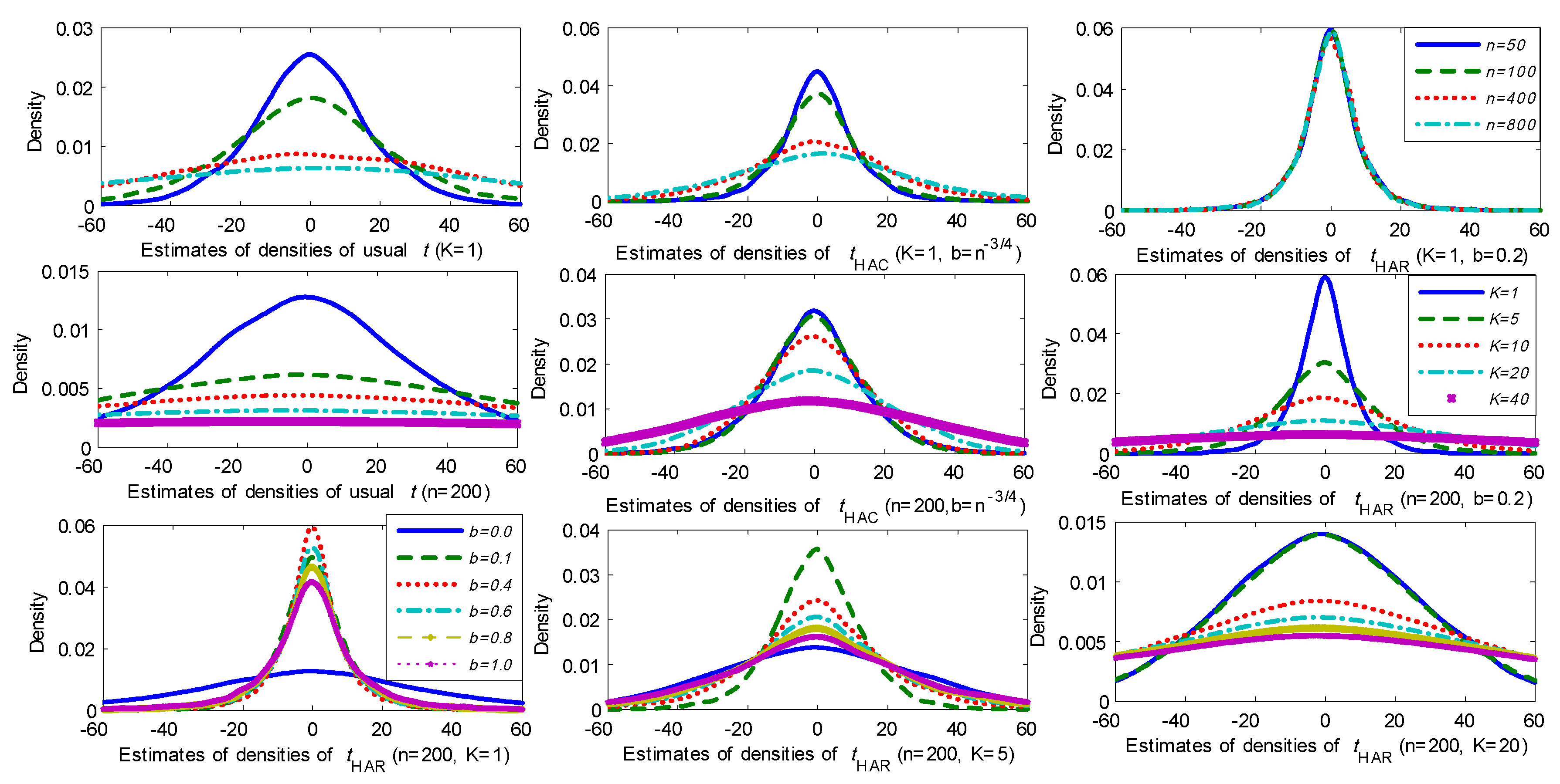
Figure 1 reports the kernel estimates of the probability densities for these t-statistics under different model scenarios based on 10,000 simulations. The first row of graphs in Figure 1 gives the results for the different t-statistics as the sample size n increases with fixed $K=1$. It is evident that both the usual t-statistic and HAC t-statistic (with $M=⌊nb⌋$ and $b=n^{-3/4}$) diverge as n increases and the HAC statistic diverges at a slower rate. In contrast, the HAR t-statistic ($b=0.2$) is evidently convergent to a well-defined probability distribution as the sample size expands. These results clearly corroborate Theorem 1.

The second row of graphs in Figure 1 presents the estimated densities of the three t-statistics as K increases for a fixed sample size $n=200$. As K increases, all three t-statistics are clearly divergent but at different rates. For each statistic the increase in dispersion as K increases is evident. The last row reports the results for the HAR t-statistic with $K=1,5,20$ and bandwidth coefficient $b=0,0.1,0.4,0.6,0.8,1$. As K increases while maintaining the same bandwidth setting, the densities become more progressively dispersed. For fixed K, it is clear that the quantile is not a monotonic function of b. For $K=1,5$, when b is close to zero, the limiting distributions become more dispersed. When b is close to one, the limiting distributions also get dispersed for all three choices of K. As explained in (Sun 2004), for small or moderate K, when b is close to zero, the behavior of the t-statistic may be better captured by conventional limit theory without taking into account the persistence of the regression residuals. But when b is close to unity, we can not expect the standard variance estimate to capture the strong autocorrelation. If we choose the kernel $k\left(x\right)=1$ and use the full sample (i.e., setting $b=1$), the long run variance estimate equals zero by construction. We conjecture that for fixed K it may be possible to find an optimal bandwidth $b_{opt}\left(K\right)$ by following an approach similar to the method used in (Sun et al. 2011) that controls for size and power. From the shape of the densities in the last row of graphs in Figure 1, we would expect that any such optimal bandwidth $b_{opt}\left(K\right)$ will get closer to zero as K gets larger. Extension of robust testing techniques to machine learning regressions where K may be very large will likely require very careful bandwidth selection in significance testing that takes the magnitude of K into account.

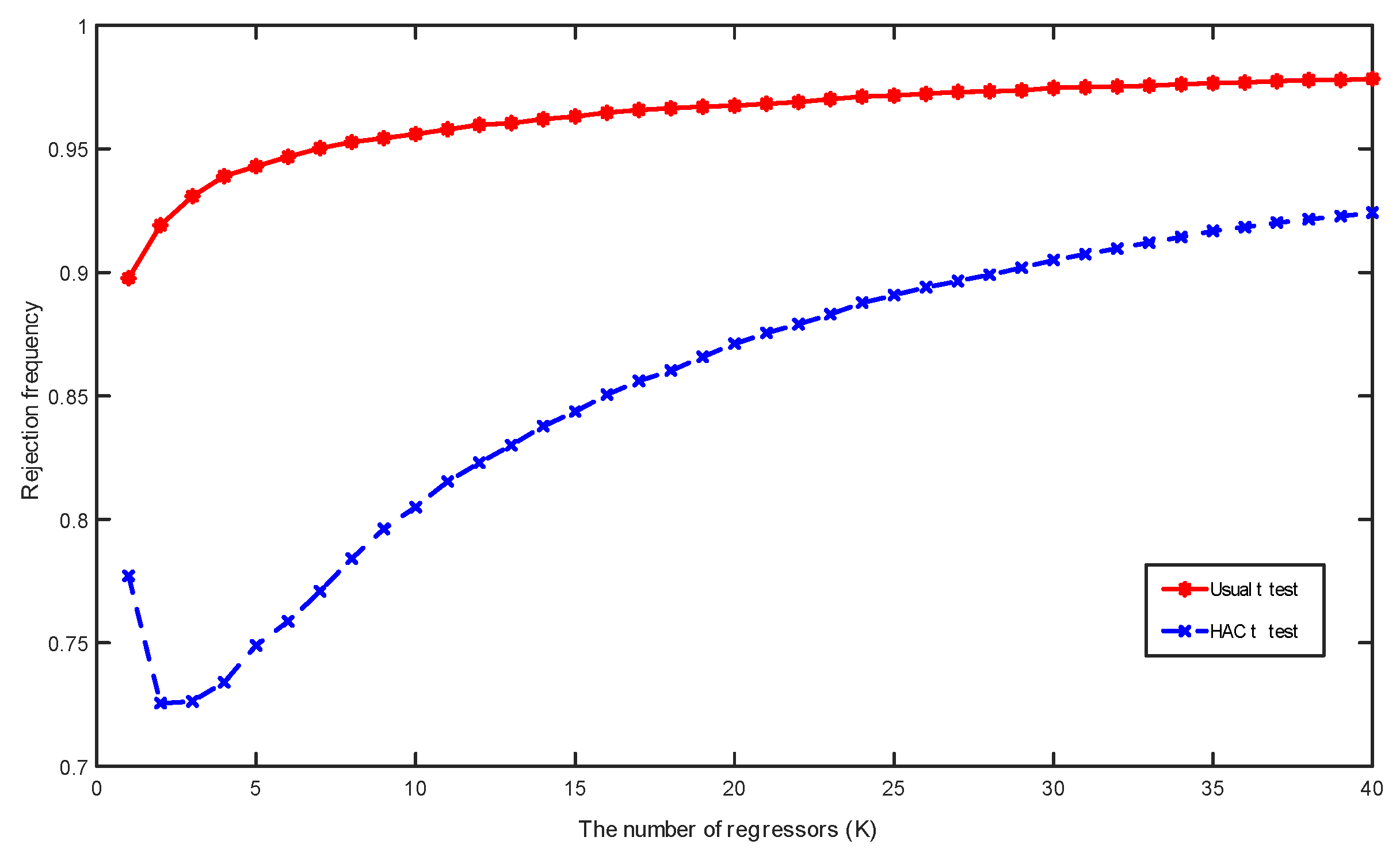
Figure 2 and Figure 3 present rejection frequencies of the three t-statistics in spurious trending regression when conventional critical values from the standard normal distribution at the 5% significance level are used. These frequencies are calculated based on 10,000 simulations with the sample size $n=200$. A manifest feature in Figure 2 and Figure 3 is that the rejection frequencies increase faster towards one as the number of regressors K increases. This feature corroborates Theorem 2 and the simulation results in Figure 1, which reveal the progressive dispersion of the densities of the three t-statistics as K increases, suggesting that the rejection frequencies are increasing functions of K for each test.

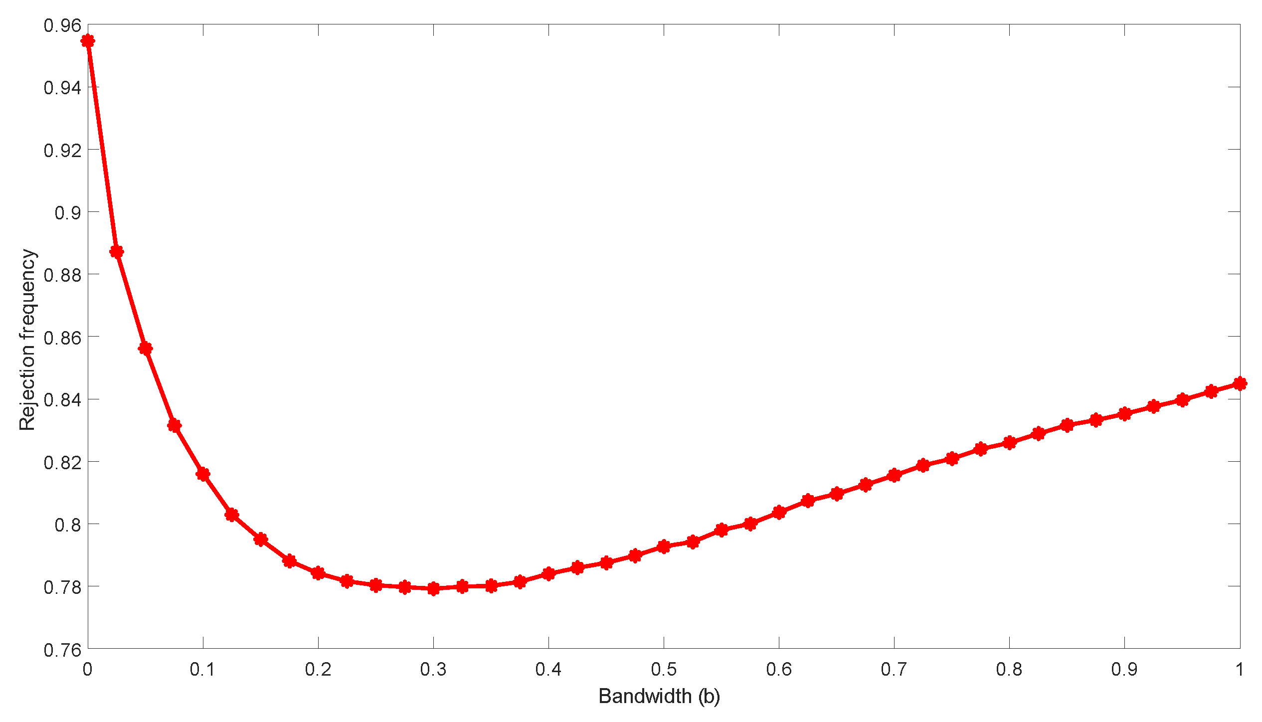
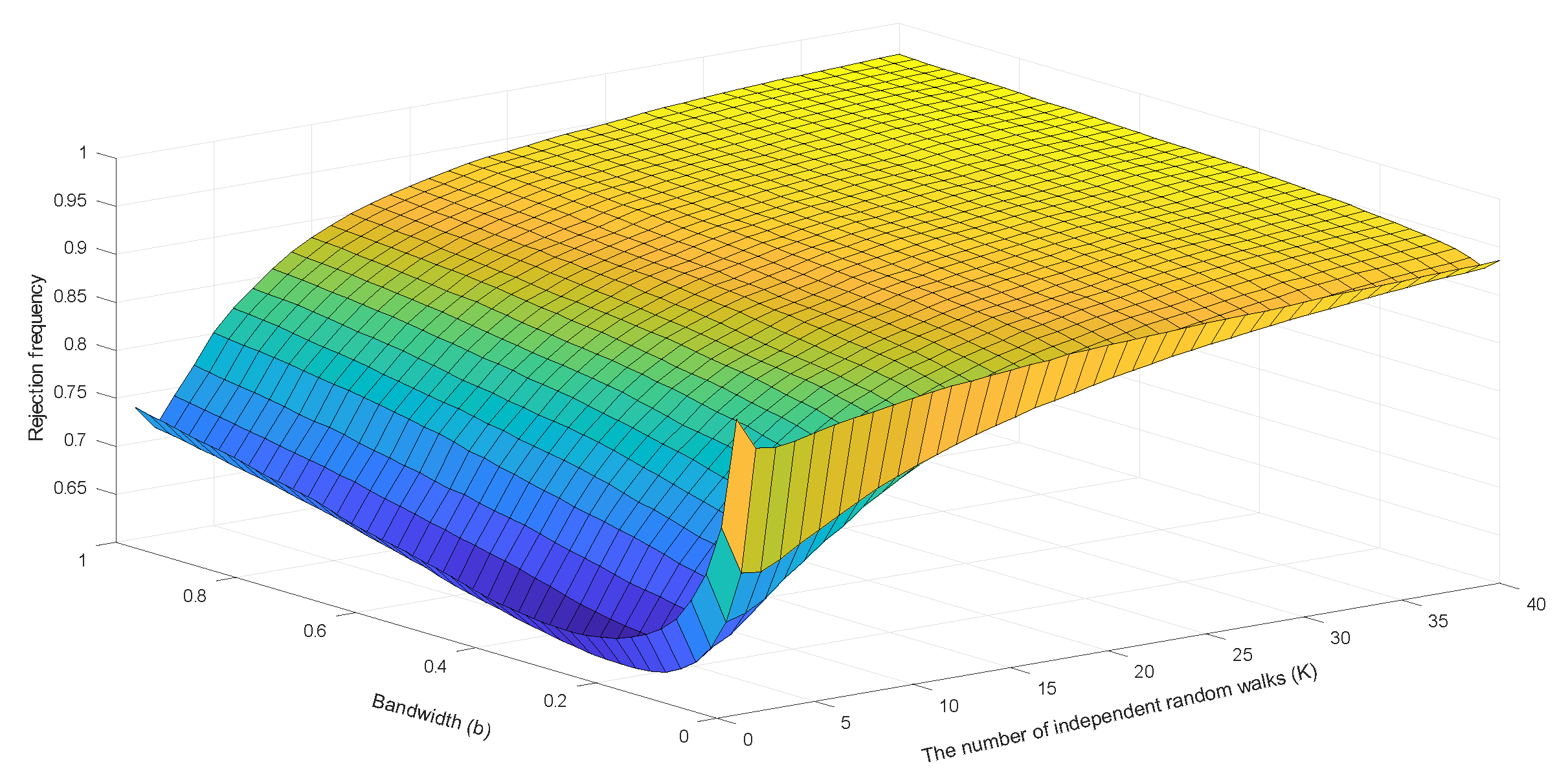
The surface displayed in Figure 3 also reveals the effect of the bandwidth choice on the rejection frequencies of the HAR test, in which the bandwidth b varies from 0 to 1 at step length 0.025. It is evident that the rejection frequency of the HAR test is a nonlinear function of b, especially when K is small. Optimal selection of a bandwidth $b_{opt}\left(K\right)$ that controls size and power of the HAR test is therefore possible. The value of $b_{opt}\left(K\right)$ should moderately deviate from zero when K is small and move towards zero faster as K increases. The findings in Figure 3 support the conjecture about the optimal bandwidth choice, which was discussed above based on the results in Figure 1.

Next, we consider a simple spurious linear trend regression of $X_t$ on a linear time trend $t,$ where $X_t={\sum }_{s=1}^t{\mu }_s$ and $u_s{\sim }_{d}iid$$N\left(0,1\right)$. Figure 4 reports the sampling densities for different t-statistics based on 10,000 simulations. The first row of graphs presents kernel estimates of densities of the t-statistics for sample sizes $n=50,100,400,800$. Again, the usual t-statistic and HAC statistic are divergent but at different rates. The HAR statistic is evidently convergent. The second row in Figure 4 provides results for the HAR statistic with different bandwidth choices. It is clear that the distributions become more dispersed as b moves close to zero or close to one. In this respect the findings are similar to those of Figure 1 when $K=1$. In Figure 5, the rejection frequencies of the HAR statistic with various bandwidth values are reported, which are calculated based on 10,000 simulations with sample size n = 200 and critical values from the standard Normal distribution at 5% significance level. Rejection frequency again follows a U-shaped function of b. This curve suggests that, for simple spurious linear trend regression, the value of the optimal bandwidth should be around 0.3.

Last, we consider spurious regressions of a standard Gaussian random walk process ${\left\{X_t\right\}}_{t=1}^T$ on independent Gaussian random walks ${\left\{Z_t\right\}}_{t=1}^T$, where $X_t={\sum }_{s=1}^t{\mu }_s$ with $u_s{\sim }_{d}iid$$N\left(0,1\right)$ and $Z_t={\sum }_{s=1}^t{\mu }_s^{\left(z\right)}$ with ${\mu }_s^{\left(z\right)}{\sim }_{d}iid$$N\left(0,I_K\right).$ Figure 6 shows kernel estimates of the probability densities for these t-statistics under different scenarios based on 10,000 simulations. Figure 7 and Figure 8 report the simulated rejection frequencies of these t-statistics for various values of K and b. The patterns exhibited are evidently similar to those in Figure 1, Figure 2 and Figure 3. The same qualitative observations made for Figure 1, Figure 2 and Figure 3 therefore apply to these regressions.

5. Conclusions

Robust inference in trend regression poses many challenges. Not least of these is the critical difficulty that a trending time series trajectory can be represented in a coordinate system by many different functions, be they relevant or irrelevant, stochastic or non-stochastic. Valid significance testing in this context needs to allow for the fact that trend regression formulations inevitably fail to capture all the subtleties of reality and to a greater or lesser extent, therefore, involve some spurious components. The practical implications of this message are powerfully stated in the header by David Hendry that opens this article.

The present work has studied the asymptotic and finite sample performance of simple t statistics that seek to achieve some degree of robustness to misspecification in such settings. The analysis is based on three classic examples of spurious regressions, including regression of stochastic trends on time polynomials, regression of stochastic trends on a simple linear trend, and regression among independent random walks. Concordant with existing theory, the usual t-statistic and HAC standardized t-statistic both diverge and imply ‘nonsense relationships’ with probability going to one as the sample size tends to infinity. Also concordant with existing theory, when the number of regressors K is fixed, the HAR standardized t-statistics converge to non-degenerate distributions free from nuisance parameters, thereby controlling size and leading to valid significance tests in these spurious regressions. These findings reinforce the optimism expressed in earlier work that fixed-b methods of correction may fix inference problems in spurious regressions.

But when the number of trend regressors $K\to \infty$, the results are different. First, rates of divergence of the usual t-statistic and HAC t-test are greater by the factor $\sqrt{K}$ than when K is fixed. Second, the fixed-b HAR t-statistic is no longer convergent and instead diverges at the rate $\sqrt{K},$ leading to spurious inference of significance when $K\to \infty$. Thus, in the case of models with expanding regressor sets, none of these standard statistics produce valid consistent tests with controllable size. The failure of the HAR test in this setting is particularly important, given the growing use of machine learning algorithms in econometric work where large numbers of regressors are a normal feature in initial specifications. Future research might usefully focus on methods of controlling size and achieving consistent significant tests in such settings. A further area of research that is relevant in practical work involves extension of the present results to regressions that involve more general forms of stochastic trend processes, including higher-order integrated and fractionally integrated processes, as well as unbalanced regressions. The methods of the present paper should be useful in developing asymptotic analyses of such potentially spurious regressions.

References

- Banerjee, Anindya, Juan J. Dolado, John W. Galbraith, and David Hendry. 1993. Co-Integration, Error Correction, and the Econometric Analysis of Non-Stationary Data. Oxford: Oxford University Press. [Google Scholar]
- Csörgö, Miklós, and Lajos Horváth. 1993. Weighted Approximations in Probability and Statistics. New York: Wiley. [Google Scholar]
- Durlauf, Steven N., and Peter C. B. Phillips. 1988. Trends versus random walks in time series analysis. Econometrica 56: 1333–54. [Google Scholar] [CrossRef]
- Eicker, Friedhelm. 1967. Limit theorems for regression with unequal and dependent errors. In Proceedings of the Fifth Berkeley Symposium on Mathematical Statistics and Probability. Beijing: Statistics, vol. 1, pp. 59–82. [Google Scholar]
- Ernst, Philip A., Larry A. Shepp, and Abraham J. Wyner. 2017. Yule’s “nonsense correlation” solved! Annals of Statistics 45: 1789–809. [Google Scholar] [CrossRef] [Green Version]
- Granger, Clive W. J., and Paul Newbold. 1974. Spurious regressions in econometrics. Journal of Econometrics 74: 111–20. [Google Scholar] [CrossRef] [Green Version]
- Hendry, David F. 1980. Econometrics—Alchemy or science. Economica 47: 387–406. [Google Scholar] [CrossRef]
- Huber, Peter J. 1967. The behavior of maximum likelihood estimates under nonstandard conditions. In Proceedings of the Fifth Berkeley Symposium on Mathematical Statistics and Probability. Beijing: Statistics, vol. 1, pp. 221–33. [Google Scholar]
- Hwang, Jungbin, and Yixiao Sun. 2018. Simple, robust, and accurate F and t tests in cointegrated systems. Econometric Theory 34: 949–84. [Google Scholar] [CrossRef] [Green Version]
- Jansson, Michael. 2004. The error in rejection probability of simple autocorrelation robust tests. Econometrica 72: 937–46. [Google Scholar] [CrossRef]
- Kiefer, Nicholas M., and Timothy J. Vogelsang. 2002a. Heteroskedasticity-autocorrelation robust testing using bandwidth equal to sample size. Econometric Theory 18: 1350–66. [Google Scholar] [CrossRef]
- Kiefer, Nicholas M., and Timothy J. Vogelsang. 2002b. Heteroskedasticity-autocorrelation robust standard errors using the bartlett kernel without truncation. Econometrica 70: 2093–95. [Google Scholar] [CrossRef]
- Kiefer, Nicholas M., and Timothy J. Vogelsang. 2005. A new asymptotic theory for heteroskedasticity-autocorrelation robust tests. Econometric Theory 21: 1130–64. [Google Scholar] [CrossRef] [Green Version]
- Kiefer, Nicholas M., Timothy J. Vogelsang, and Helle Bunzel. 2000. Simple robust testing of regression hypotheses. Econometrica 68: 695–714. [Google Scholar] [CrossRef]
- Lazarus, Eben, Daniel J. Lewis, James H. Stock, and Mark W. Watson. 2018. HAR inference: Recommendations for practice. Journal of Business & Economic Statistics 36: 541–59. [Google Scholar]
- Loève, Michel. 1963. Probability Theory, 3rd ed. New York: Van Nostrand. [Google Scholar]
- Müller, Ulrich K. 2007. A theory of robust long-run variance estimation. Journal of Econometrics 141: 1331–52. [Google Scholar] [CrossRef] [Green Version]
- Müller, Ulrich K. 2014. HAC corrections for strongly autocorrelated time series. Journal of Business & Economic Statistics 32: 311–22. [Google Scholar]
- Müller, Ulrich K., and Mark W. Watson. 2016. Low-frequency econometrics. In Advances in Economics: Eleventh World Congress of the Econometric Society. Edited by Bo Honoré and Larry Samuelson. Cambridge: Cambridge University Press, vol. 2, pp. 53–94. [Google Scholar]
- Müller, Ulrich K., and Mark W. Watson. 2018. Long-run covariability. Econometrica 86: 775–804. [Google Scholar] [CrossRef]
- Park, Joon Y., and Peter C. B. Phillips. 1988. Statistical inference in regressions with integrated processes: Part 1. Econometric Theory 4: 468–97. [Google Scholar] [CrossRef] [Green Version]
- Park, Joon Y., and Peter C. B. Phillips. 1989. Statistical inference in regressions with integrated processes: Part 2. Econometric Theory 5: 95–131. [Google Scholar] [CrossRef] [Green Version]
- Phillips, Peter C. B. 1986. Understanding spurious regression in econometrics. Journal of Econometrics 33: 311–40. [Google Scholar] [CrossRef] [Green Version]
- Phillips, Peter C. B. 1991. Optimal inference in cointegrated systems. Econometrica 59: 283–306. [Google Scholar] [CrossRef] [Green Version]
- Phillips, Peter C. B. 1996. Spurious regression unmasked. In Cowles Foundation Discussion Paper. No. 1135. New Haven: Yale University. [Google Scholar]
- Phillips, Peter C. B. 1998. New tools for understanding spurious regressions. Econometrica 66: 1299–325. [Google Scholar] [CrossRef]
- Phillips, Peter C. B. 2002. New unit root asymptotics in the presence of deterministic trends. Journal of Econometrics 111: 323–53. [Google Scholar] [CrossRef] [Green Version]
- Phillips, Peter C. B. 2005. HAC estimation by automated regression. Econometric Theory 21: 116–42. [Google Scholar] [CrossRef] [Green Version]
- Phillips, Peter C. B. 2014. Optimal estimation of cointegrated systems with irrelevant instruments. Journal of Econometrics 178: 210–24. [Google Scholar] [CrossRef] [Green Version]
- Phillips, Peter C. B., and Steven N. Durlauf. 1986. Multiple time series regression with integrated processes. Review of Economic Studies 55: 473–96. [Google Scholar] [CrossRef] [Green Version]
- Phillips, Peter C. B., and Bruce E. Hansen. 1990. Statistical inference in instrumental variables regression with I(1) processes. Review of Economic Studies 57: 99–125. [Google Scholar] [CrossRef]
- Phillips, Peter C. B., and Mico Loretan. 1991. Estimating long-run economic equilibria. Review of Economic Studies 59: 407–36. [Google Scholar] [CrossRef] [Green Version]
- Phillips, Peter C. B., and Zhentao Shi. 2019. Boosting the Hodrick-Prescott filter. In Cowles Foundation Discussion Paper. No. 2192. New Haven: Yale University. [Google Scholar]
- Phillips, Peter C. B., and Victor Solo. 1992. Asymptotics for linear processes. The Annals of Statistics 20: 971–1001. [Google Scholar] [CrossRef]
- Robinson, Peter M. 1998. Inference-without-smoothing in the presence of nonparametric autocorrelation. Econometrica 66: 1163–82. [Google Scholar] [CrossRef]
- Sun, Yixiao. 2004. A convergent t-statistic in spurious regression. Econometric Theory 20: 943–62. [Google Scholar] [CrossRef] [Green Version]
- Sun, Yixiao. 2014a. Let’s fix it: Fixed-b asymptotics versus small-b asymptotics in heteroscedasticity and autocorrelation robust inference. Journal of Econometrics 178: 659–77. [Google Scholar] [CrossRef]
- Sun, Yixiao. 2014b. Fixed-smoothing asymptotics in a two-step GMM framework. Econometrica 82: 2327–70. [Google Scholar] [CrossRef]
- Sun, Yixiao. 2014c. Fixed-smoothing asymptotics and asymptotic F and t tests in the presence of strong autocorrelation. In Essays in Honor of Peter C. B. Phillips (Advances in Econometrics, Volume 33). Bingley: Emerald Group Publishing Limited, pp. 23–63. [Google Scholar]
- Sun, Yixiao. 2018. Comments on “HAR inference: Recommendations for practice”. Journal of Business & Economic Statistics 36: 565–68. [Google Scholar]
- Sun, Yixiao, Peter C. B. Phillips, and Sainan Jin. 2011. Power maximization and size control in heteroskedasticity and autocorrelation robust tests with exponentiated kernels. Econometric Theory 27: 1320–68. [Google Scholar] [CrossRef] [Green Version]
- White, Halbert. 1980. A heteroskedasticity-consistent covariance matrix estimator and a direct test for heteroskedasticity. Econometrica 48: 817–38. [Google Scholar] [CrossRef]
- White, Halbert. 1982. Asymptotic Theory for Econometricians, 1st ed. Cambridge: Academic Press. [Google Scholar]
- Yule, G. Udny. 1926. Why do we sometimes get nonsense correlations between time series? A study in sampling and the nature of time series. Journal of the Royal Statistical Society 89: 1–63. [Google Scholar] [CrossRef]