Simultaneous Indirect Inference, Impulse Responses and ARMA Models †

1
Department of Economics, Room C-870 Loeb Building, Carleton University, 1125 Colonel By Drive, Ottawa, ON K1S 5B6, Canada
2
Canada Mortgage and Housing Corporation, Homeowner Risk Management, Strategy and Products, 700 Montreal Road, Ottawa, ON K1A 0P7, Canada
*
Authors to whom correspondence should be addressed.
†
This work was supported by the Social Sciences and Humanities Research Council of Canada and the Fonds de recherche sur la société et la culture (Québec).
Econometrics 2020, 8(2), 12; https://doi.org/10.3390/econometrics8020012
Submission received: 19 December 2018
/
Revised: 11 February 2020
/
Accepted: 26 February 2020
/
Published: 2 April 2020
(This article belongs to the Special Issue Resampling Methods in Econometrics)
Abstract
:A two-stage simulation-based framework is proposed to derive Identification Robust confidence sets by applying Indirect Inference, in the context of Autoregressive Moving Average (ARMA) processes for finite samples. Resulting objective functions are treated as test statistics, which are inverted rather than optimized, via the Monte Carlo test method. Simulation studies illustrate accurate size and good power. Projected impulse-response confidence bands are simultaneous by construction and exhibit robustness to parameter identification problems. The persistence of shocks on oil prices and returns is analyzed via impulse-response confidence bands. Our findings support the usefulness of impulse-responses as an empirically relevant transformation of the confidence set.
1. Introduction
Indirect inference refers to resampling-based statistical methods that use simulations to calculate estimating functions including likelihoods, scores or moments. The idea of replacing complicated or intractable statistical functions by computer simulations motivated initial applications and underlying theory; see Smith (1993); Gouriéroux et al. (1993); Gouriéroux and Monfort (1996) and Gallant and Tauchen (1996). Since then, available evidence suggests that indirect inference often works better than traditional methods in finite samples for bias or misspecification corrections under various situations.1 We propose a two-stage framework that can yield identification robust confidence sets via Indirect Inference for finite samples. The primary focus concerns inference in Autoregressive Moving Average (ARMA) models and production of simultaneous confidence bands from its impulse-response functions.2
Despite the simplicity of ARMA models in time series, identification and boundary issues raise enduring complications for estimation and inference. First, Autoregression (AR) unit roots cause the so-called non-uniform convergence problem, which means that methods requiring stationarity break down at, or close to the unit boundary, whereas local-to-unity motivated methods perform poorly away from unity; see Hansen (1999); Mikusheva (2007); Andrews and Guggenberger (2010); Gorodnichenko et al. (2012); Mikusheva (2012, 2014) and Phillips (2014). Second, identification failure related to the invertibility of Moving Average (MA) components causes the so-called pile up effect, since estimating functions, including likelihoods, can have a local maximum at the invertibility boundary even when the true process is invertible; see Sargan and Bhargava (1983); Davis and Dunsmuir (1996); Gospodinov (2002); Genton and Ronchetti (2003); Billio and Monfort (2003); Davis and Song (2011); and Gospodinov and Ng (2015).
Third, root cancelation, also known as common factors, or parameter redundancy described, e.g., in Harvey (1981), occurs when the AR polynomial and the MA polynomial have one or more roots in common. Root cancelation and near-root cancelation produce spurious inference related to lack of identification or weak-identification of the parameters in question. Identification and inference concerns in this context have been extensively analyzed in the literature. For instance, Ansley and Newbold (1980) document the severe bias suffered by the Maximum Likelihood Estimation (MLE) for finite samples. Galbraith and Zinde-Walsh (1997) and references therein focus on providing identification devices for ARMA models. Nelson and Startz (2007) emphasize that near-root cancelations lead to spurious inference regardless of large sample sizes, even when asymptotic theory is expected to hold. More recently, see Andrews and Cheng (2012) and Andrews and Mikusheva (2014, 2015), most of which remains asymptotic.
Our two-stage simulation approach complements the asymptotic frameworks available in the literature, in the sense that it presents a finite sample version; see Khalaf and Saunders (2019). Indirect Inference relies on a binding function that links parameters of interest to auxiliary parameters, for which simple estimators are available. The binding function admits a simulation-based approximate. Hence, we propose the following Ordinary Least Squares (OLS) auxiliary estimates: (i) least squares in two-sided regressions with leads and lags, (ii) least squares in long-autoregressions (AR), and (iii) empirical autocorrelations. Methods with leads and lags generally aim to deal with feedback effects; see Stock and Watson (1993); Dufour and Torres (2000). AR-based approximations have long been popular for ARMA models; see Hannan and Rissanen (1982); Galbraith and Zinde-Walsh (1994, 1997); Ghysels et al. (2003); Guay and Scaillet (2003); Gospodinov and Ng (2015); Dufour and Pelletier (2014). Empirical autocorrelations and related measures including cumulants and local projections have recently been re-introduced from a minimum distance perspective; see e.g., Jorda and Kozicki (2011); Gorodnichenko et al. (2012); Gospodinov and Ng (2015) and references therein. Our two-stage simulation framework unifies all the above for confidence interval purposes.
The first simulation stage involves constructing a Wald-type minimum-distance metric that matches auxiliary parameters with corresponding estimates. Typically in Indirect Inference, standard asymptotic arguments are employed to derive confidence sets and hypothesis tests; however, these assume that parameters are identified. In contrast to the standard extremum extimation strategy, we propose to treat this Wald-type distance metric as a test statistic, which we invert, rather than minimize. Inverting a test involves collecting the values of the parameter that are not rejected via this test at a given level of significance to construct a confidence set. Exactness and identification robustness are achieved by applying the Monte Carlo (MC) test method from Dufour (2006) to compute simulated p-values in a second stage. This method achieves size control 3 when the null distribution of the statistic, even if not computable analytically, does not depend on unknown or nuisance parameters.4 In our ARMA application, a nuisance-parameter-free distribution results from scale-invariance of OLS in AR settings, and from the standardization inherent to empirical autocorrelations. Laslty, the confidence set is projected to construct impulse-response confidence bands, which entails maximizing and minimizing each function over the non-rejected values of the parameters. The confidence intervals obtained are thus simultaneous by construction and robust to the aforementioned identification problems.
We conduct a simulation study on ARMA and MA processes and compare our method with MLE-based inference. Simple objective functions as in Galbraith and Zinde-Walsh (1994, 1997), as well as over-identified criteria are considered, in addition to various lag structures. Results can be summarized as follows. In contrast to MLE, our method eradicates pile up root cancelation problems and boundary problems, even with very small samples, with no more than 50 observations. MLE is oversized for both individual parameter and joint tests. None of the estimation functions steadily outperforms the rest for all sample sizes and pairs tested. Thus, we incorporate a joint criterion, constructed by averaging the three proposed objective functions, to exploit the power advantages of each of them. Leads improve power for highly persistent processes. Overidentification yields important power benefits. On balance, autocorrelation-based methods require a larger sample to catch up power-wise with AR-based counterparts. Inverting the asymptotic Wald test based on MLE estimates is almost infeasible at corner solutions with parameters close to the unit boundary, since in many instances the variance-covariance matrix is not invertible. This result is expected and provides support to our research.
Our methodology is applied with a univariate perspective to investigate the persistence of oil shocks via impulse-responses confidence bands. We select daily spot prices of the West Texas Intermediate (WTI), a high quality, light sweet crude oil, delivered at Cushing, Oklahoma and priced in U.S. dollars per barrel. We focus on the logarithmic transformation of prices and returns at the weekly and monthly frequencies. The main advantage of our method is the possibility of remaining agnostic with respect to the process followed by these series. Among our results, we highlight that our simultaneous impulse-response confidence bands seem well identified, despite the presence of parameter uncertainty in these series. We find that root cancelation does not bias our results; however it affects predictability; in particular, by obscuring the behaviour of impulse-responses for oil returns. Hence, when the focus of the analysis is on predictability, researches should favour the study on prices, instead of growth in prices. We find that shocks to oil prices are permanent, taking about a decade or so to die down. Also, relying on MLE to estimate the effect of shocks when processes are highly persistent can mislead researches when conducting estimation and forecasting. In contrast, our proposed impulse-response confidence bands represent an empirically relevant transformation of the joint confidence set.
We introduce our framework in Section 2 and discuss inference by test inversion in Section 3. The ARMA special case is presented in Section 4. Simulation results are presented in Section 5. An empirical application with focus on benchmark oil prices and returns is explored in Section 6 and we conclude in Section 7.
2. General Framework
Consider the general model
where is the sample space, such that a sample of size T is represented as
is a probability distribution over indexed by and is the parameter space. We also asume that can be partitioned as
where and are partitions of . is the q-dimensional parameter of interest and is a nuisance parameter, which we aim to partial out.
Pseudo-data can be simulated from (1) and an auxiliary parameter denoted , of dimension , can be defined in a way that it is linked to via an exact or limiting binding function, . In general, need not have a known analytical form. Furthermore, a simple statistic is available to estimate given X.
Denote by the considered data-based estimate of where is the estimating function. Its simulation-based counterpart, given a specific value of , can be derived, for example, in this way: (i) creating H simulated paths,
each of size T from (1) given ; (ii) applying the same estimation method to each simulated path, leading to a series of estimations,
and then (iii) computing their average as follows,
The distance between and forms the basis of Indirect Inference. A common special case is the Wald-type distance measure where is a positive definite weighting matrix. Gouriéroux et al. (1993) suggest where denotes a p-dimensional identity matrix because the loss in efficiency with respect to an optimal estimator can be disregarded. This practice is also suggested, more recently, by Gouriéroux et al. (2010).
2.1. Nuisance Parameters
Focusing on as the parameter of interest requires a strategy to account for . In some settings, can be easily estimated given . Alternatively, an auxiliary estimate, or objective function that is exactly invariant to can be considered. We emphasize the latter case in this study, defined via the following assumptions that characterize the model and its respective estimating functions.
Assumption 1.
In the context of model (1), an estimating function is invariant to , if
where and are samples from (1) with and respectively, and are two different values of
This assumption ensures that
which yields an invariant objective function for the transformation that maps into . Indeed, applying Assumption 1 to the calibration in (6), we have:
It follows that can be set to any value in for simulation purposes with no bearing on estimation, nor inference, via objective functions of the form
In line with the above cited literature, (10) uses an identity weighting matrix. Other choices are possible as long as remains invariant to , or the distribution of does not depend on under the null hypothesis that fixes .
A common special case includes scale invariance, which implies robustness to multiplying the data by any positive scalar a, so Assumption 1 yields the following,
which together imply:
Its multivariate counterpart involves multiplying the data by an invertible matrix. For illustrations on finite sample cases, see Beaulieu et al. (2007, 2013) and Dufour et al. (2003, 2010).
Invariance also implies that in the simulation study, can be set to any known value in its parameter space, since it will be partialled-out. Hence, we simplify our notation by supressing in , and , and redefining them as , and .
3. Inference via Test Inversion
Standard applications of Indirect Inference resort to minimizing (10) and formulating adequate regularity conditions, so that the resulting estimator, denoted , is (typically) asymptotically normal with a covariance matrix that can be estimated consistently. To compare and contrast our proposed inference method with common practices and to define test inversion within a familiar setting, let us revisit the traditional -level confidence interval,
for a given scalar function , where denotes the relevant standard error estimate computed (for example, via the delta-method) from the estimated asymptotic variance-covariance matrix of and is a two-tailed standard normal critical point. As it is well known, is derived by solving the following inequality, over :
Said differently, the solution of (15) inverts a t-type test of
based on the statistic .
The null hypothesis may also cover the full model specification in conjunction with testing , in which case, the alternative hypothesis is no longer restricted to . Interpreting rejections when the model is jointly tested calls for caution; and when such a test is inverted, the outcome may be the empty set, which indicates that the model under the null is misspecified. The test that we invert below follows these principles, in the sense that model misspecification is covered by the alternative hypothesis.
Ideally, , at least as . However, identification failures, or stationarity concerns will cause intervals of this form to severely under-cover, even with large samples. In our research, we depart from this approach and propose a confidence set for based on inverting a test of the form,
using (10), which we treat as a test statistic. Inverting a test of at a given level consists in collecting, numerically or analytically, the values that are not rejected using the considered test at the specified level. For example, given the right-tailed test statistic,
and assuming (for the moment and for illustrative purposes) that an -level cut-off point is available, the test inversion involves solving, over , the inequality . The solution of this inequality is a parameter space subset, denoted , that satisfies:
Since the finite sample distribution of (10) is intractable, and since there is no reason to expect that a cut-off point invariant to can be found, a numerical solution is required.
We propose collecting via numerical search, the values that are not rejected using a MC p-value that we will define in the next section, denoted . In other words, we propose to search for the values for which . The result is a joint -level confidence region denoted , as mentioned before. The set thus derived can be empty, which will provide a diagnostic test of the hypothesized model. Said differently, an empty confidence set would occur when all values of are rejected at the considered level, meaning that in this case, the selected specification would be incompatible with the available data. Our proposed variant of Indirect Inference preserves its specification-robustness attributes. If identification is weak, the set will be unbounded or diffuse, which will also provide useful information regarding model fit (or lack thereof).
If a confidence interval for the individual components of or, more generally, for a given function is desired, the above defined can be projected. This implies minimizing and maximizing over the values in . We study a special case of ARMA-based impulse-response functions that illustrates the usefulness of such projections.
3.1. Exact p-Values
We propose applying Dufour’s (2006) MC method to compute the above empirical p-value.Given that the null distribution of the considered statistic is nuisance parameter free, the MC method controls the type I error even if is itself simulation-based, in finite samples. This method is summarized as follows.
First, we introduce a new layer of simulation, for each value of : We draw L replications satisfying the null hypothesis in (17) from the model,
These replications should be generated independently from the simulations underlying . Next, we apply to each replication l leading to
and compute a series of statistics that are similar to the one in (18), but now considering the vector of the estimated parameters obtained from , for each replication l,
instead of the vector obtained by applying the estimation method to the data. We are able to use the same vector of calibrated parameters, from (18), due to the exchangeability property of the MC test; see Dufour (2006). Lastly, the empirical p-value associated with the null hypothesis is computed as
where denotes the number of times the statistic is greater than or equal to the data-based statistic 5
4. ARMA Special Case
We consider the zero mean Gaussian ARMA(1,1) process of size T with unknown parameters ,
with
where guarantees invertibility or an Autoregressive AR(∞) representation, ensures stationarity in causal processes and the joint distribution of is known. For example, can be assumed independent and identically distributed with a standard normal distribution:
This notation implies that is the pre-sample observation (i.e., it is not observed), in which case further assumptions are needed due to our indirect inference focus. In a stationary 6 environment, should be set to the following:
Alternatively, can be set to zero, which maintaining (27), fixes to zero.
Gaussian and Student- errors are considered in our Monte Carlo (MC) simulations and empirical application; the generalized lambda family of distributions as considered in Gospodinov and Ng (2015) is another interesting parametrization. Non-zero mean and exogenous variables can be projected out. With regards to the above notation, we maintain as the nuisance parameter and we focus on inverting tests as in (17), for .
In this context, for any positive scalar a and number of lags p, we have:
and
These invariance properties guarantee that the argument that minimizes would numericly coincide if the data generating process (DGP) is drawn with unit variance or any other value of ; the same holds for the empirical autocorrelations. To simplify the notation, we use the same number of leads and lags in , although clearly, invariance to does not require this restriction. The choice in terms of the number of lags p is user defined, as it is the case with all auxiliary model-based methods. In contrast to most existing methods, the methodology that we propose controls the significance level for any given p and thus regardless of the truncation order. This is discussed further in the context of our simulation study in Section 5.
Conformably, we consider three choices for our estimating function : (i) two -sided OLS estimation with forward and backward-looking components; (ii) OLS estimation of backward-looking or long-AR; and (iii) empirical autocorrelations. For clarity, and given any sample vector of size T, we will refer to these choices as
where corresponds to (28) and is given by (31).
For each choice of the estimating function, we construct a test statistic considering the distance between the previously estimated and the simulation-calibrated auxiliary parameters. In addition, to be able to harvest all available information, we construct a fourth test statistic by a simple average of those three.
Because we focus on an invariant auxiliary statistics, to compute their simulation-based counterparts for any given value of the parameters, it suffices to create H simulated paths, , as
Population autocorrelations need not be derived by simulation; yet invariance is explicitly imposed this way for any p. For the MA(1) special case, we also use a simplified auxiliary parameter: We fit a long-AR to observed and simulated data and retain the coefficient of the first lag .
4.1. Impulse-Response Confidence Bands
Impulse-response functions are the most empirically and policy relevant transformations of ARMA parameters. If the stationarity condition is satisfied, (24) admits an MA (∞) approximation using lags operators L,
and the empirical impulse-response coefficients can be computed following the well-known iterative process:
These equations define a series of known functions of the vector , denoted , m, that can be projected in turn, which imply minimizing and maximizing over the values in .
Resulting confidence intervals are simultaneous, in the following sense. Let denote the image of by the function . Then, (19) implies that
The simulation study reported below includes an illustrative analysis of such projections emphasizing close to boundary values of the MA parameter and the AR parameter , as well as robustness to root cancelation.
5. Simulation Study
We conduct MC simulation experiments to assess the performance of our method for MA(1) and ARMA(1,1) processes. Our objective is to study power and size when MA parameters are close to the non-invertibility region for both processes, and the AR parameter is close to the non-stationary region for the ARMA. Our experiments are designed as follows. Simulated samples with number of observations T equal to 50, 100 and 200, used here as pseudo-data, are drawn from the ARMA model in (24). First, time series of errors are drawn from a Gaussian, or a Student-t distribution with 5 degrees of freedom, setting , in line with Assumption . These choices of sample size correspond to samples employed in other MC studies, as well as data used in empirical applications.
The dimension of the auxiliary parameter is assessed by simulation. Power is studied by selecting various combinations of number of parameters and paths within the simulations explored in our model. Various tests are performed by changing the number of auxiliary parameters in our experiments -refer to definitions in Section 2- from 1 to 3 and 8 for the MA and from 6 to 8 and 12 for the ARMA. We take into consideration the recommendations from Galbraith and Zinde-Walsh (1994) and Ghysels et al. (2003) for the long-AR estimation, and Gorodnichenko et al. (2012) for the estimation with autocorrelations. We find that selecting 8 auxiliary parameters provides the highest power for all the sample sizes. 7 Hence, we suggest that for empirical practices, the total number of auxiliary parameters is set to 8 for each of the choices of the estimating functions, explained in Section 4: (i) in the OLS estimation with forward and backward-looking components, (ii) in the OLS estimation of the long-AR, and (iii) in the estimation with empirical autocorrelations. In the case of the simplified auxiliary parameter estimation for the MA process, the long-AR is estimated with 8 parameters, but only the first coefficient is retained.
As part of previous experiments, we test the number of simulated paths in the first simulation stage, setting and , as suggested by Ghysels et al. (2003) for the MA, and also , to examine whether it could improve power for ARMA -refer to the notation in Section 2. However, is finally selected, keeping the number of auxiliary parameters equal to 8, as the value which provides the highest power for all sample sizes. The number of replications in the second simulation step, involving the application of Dufour’s (2006) MC method, is and we consider a level of significance -see notation in Section 3. An identity weighting matrix is used to preserve the invariance to scale of the statistic associated to every choice of the estimating function. Lastly, 1000 replications are considered on each MC simulation experiment.
5.1. Main Results
Each pair of parameters employed in the data generating process (DGP) of ARMA(1,1) is denoted in our experiments as . Outcomes from all our simulation studies are available upon request. We focus on the following set of pairs to illustrate our results: . Note that we set the AR parameter equal to zero in (24) a priory to draw samples from MA(1) processes, for instance, when the value of is 0.6 and 0.99.
We report power in terms of empirical rejections and our main results are summarized along the following lines. The results of the experiments conducted for MA(1) processes are presented in Table 1 and Table 2, and the studies related to the ARMA(1,1) process are shown in Table 3 and Table 4. We use abbreviations for each estimating function: OLS-FBLC, OLS-Long AR and AutoCorr correspond to the OLS estimation with forward and backward-looking components, the OLS estimation of the long-AR and the estimation with empirical autocorrelations, respectively. Size is controlled with our method for all sample sizes, choices of the estimating function, and for both Gaussian and Student- t errors, irrespective of how close the true parameters are to the unit root. It is well known that MLE gives size distortions when the sample size is small, for both, individual parameter tests and joint tests. Size seems to improve for the MLE when the sample size is increased and the parameters are far from the unit root regions. However, when the parameters approach the unit root regions, size fails for the MLE as the sample size increases, which confirms its asymptotic failure.8
Results obtained in term of power for processes with Student- t errors are in line with the ones obtained with Gaussian errors. This outcome confirms the robustness of our framework to fatter tails, since we purposely ignore the fact that the errors are drawn from the Student- t distribution when we apply our method.
Table 1 and Table 2 exhibit results from experiments on MA processes. The top section of this table compares our method -denoted SIM METHOD in the tables- versus MLE in terms of size. Note that MLE is oversized, while size remains exact for our method. We can identify that the pile up effect starts for values of the parameter higher than 0.6, in finite samples. Although our method does not produce size distortions, it cannot discriminate between tested values higher than 0.85, when the true DGP value is between 0.85 and 1. This result is expected and traced back to, e.g., Stock (1991) and references therein. Typically, when values of the parameter near the boundary (around 0.99) cannot be refuted, values substantially different (for instance, 0.85) from the boundary are also hard to refute in small samples. For small values of the parameter, the method with the simplified auxiliary parameter estimation, inspired in Galbraith and Zinde-Walsh (1994, 1997), shows an increase in power with respect to the OLS estimation of the long-AR. However, as the tested value of the parameter increases and gets closer to the unit root region, the latter method shows higher power than the former. This result indicates that overidentification is useful to increase power when we have higher persistence in MA(1) processes.
In general, the power of our method increases for the three estimating functions applied to the ARMA as the sample size increases, but none of them steadily shows the highest power for all sample sizes and pairs tested. When the AR parameter is closer to the unit root than the MA parameter and the sample is very small, 50 or 100 observations, our method applied with the OLS estimation with forward and backward looking components offers the highest power on the boundary. However, when the reverse occurs, the MA parameter is closer to the unit root than the MA parameter, our framework with the autocorrelations enables better discrimination between the true pair and any pair with values that are closer to the boundaries. Results obtained with the root cancelation pair, are reported in Table 3. As before, the top section of the table compares our method versus MLE in terms of size. Size remains exact for our method in this case; however MLE is oversized. When the OLS estimation with forward and backward components is applied, it gives the highest power for almost all the pairs tested for a sample size of T = 50 observations. Once we increase the sample size to 100, this estimating function still shows the highest power, followed closely by the second choice of estimating function, the OLS estimation of the long-AR. When the sample size is T = 200, the power obtained with the autocorrelations reaches closely to the power obtained with the other two estimating functions.
Lastly, we examine the almost unit root pair as the true DGP pair, in Table 4. For most of the pairs tested, applying the method with the OLS estimation of the long-AR gives the highest power for sample sizes of T = 50 and T = 100. However, for the same sample sizes, using autocorrelations gives the highest power for the last three pairs tested, for which the value of the MA parameter is closer to the boundary than the value of the AR parameter. As we increase the sample size, power reaches similar values for our method with the three estimating functions.
5.2. Robustness Checks
In addition to our previous experiments, we conducted simple robustness checks for our method. Two examples are shown in Table 5 and Table 6. We present the power values for two ARMA processes which are misspecified as ARMA(1,1) with a sample size T = 100. In Table 5 we have an ARMA(2,1) with , so we have a high persistence AR(2) mixed with a low persistence MA(1). In general, the method applied with autocorrelations offers more power rejecting the pairs where the AR parameter is closer to the boundary than the MA parameter; while with the OLS estimation with forward and backward-looking components we obtain more power rejecting the pairs where the MA parameter is closer to the boundary than the AR parameter.
The ARMA (2,1) in Table 6 with , shows a high persistence AR(1) mixed with a MA(2), which has higher persistence on its second parameter. In this case, we find that the method applied with both, the OLS estimation of forward and backward-looking components and the OLS estimation of the long-AR, is more powerful rejecting the misspecification than with the autocorrelations. Note that in both examples, our three choices of estimating functions provide good power, rejecting the misspecification for all the pairs tested.
6. Empirical Application
Our two-stage simulation-based framework is applied with a univariate perspective to investigate the persistence of oil shocks via impulse-response confidence bands. Apart from supply and demand conditions, estimation and forecasting of oil prices are complicated by the effect of non-market related characteristics, such as, regulations, technology and geopolitical considerations; see Hamilton (1983, 1996, 2003, 2009); Kilian (2008a, 2008b, 2008c) and Kilian and Vigfusson (2017). Main concerns in the literature related to oil prices are, among others, whether the impact of oil shocks is temporary or permanent and whether a particular model can offer better performance than a random walk. Most studies support analyzing the real price of oil based on its explanatory power for macroeconomic forecasting of output, for instance, Baumeister and Kilian (2012) and Alquist et al. (2013). However, Hamilton (2011) argues that nonlinear transformations of the nominal price of oil can reflect threshold responses based on consumer sentiment. In addition, he notes that deflating nominal prices by the Consumer Price Index (CPI) introduces measurement errors that can affect forecasting results. Hence, we explore the behaviour of oil shocks considering the logarithmic transformation of prices and returns (log-differences), at the weekly frequency and also at the monthly frequency, in both, nominal and real terms.
We have identified four lines of research where oil series are characterized as a mean reverting process, in particular ARMA: (i) study of long-run persistence in oil prices, (ii) study of oil volatility persistence, (iii) DSGE calibration and (iv) application of structural Vector Autoregression (VAR) family models. The first line of research focuses on oil price dynamics with long series and makes modeling decisions considering mean reverting and random walk processes; see Pindyck (1999); Lee et al. (2006); Bernard et al. (2012); Gil-Alana and Gupta (2014). Oil volatility persistence is studied in the second line of research, either by fitting ARMA family models to volatility proxies based on transformations of oil returns, or by applying Generalized Autoregressive Conditional Heteroscedasticity (GARCH) family models directly to oil returns; see e.g., Choi and Hammoudeh (2009); Charles and Darné (2014) and references therein. In the third line of research, DSEG models frequently apply calibrations by fitting ARMA family models to oil prices, for instance, in the work of Atkeson and Kehoe (1999) and Leduc and Sill (2004). Lastly, the literature applying VAR family models is very extensive and it is mostly dedicated to forecasting in short to middle horizons; see Pindyck (2004); Kilian (2009); Alquist and Kilian (2010); Baumeister and Kilian (2012); Alquist et al. (2013); Baumeister and Kilian (2014a, 2014b), Baumeister et al. (2014); Baumeister and Kilian (2015); Baumeister et al. (2015).9 In VAR models, impulse-responses are analyzed by either applying simulations, or Bayesian methods.10
Our simultaneous analysis is related to the research of Staszewska-Bystrova (2007, 2011, 2013); Jorda (2009); Staszewska-Bystrova and Winker (2013); Jorda and Marcellino (2010); Inoue and Kilian (2013, 2016); Guerron-Quintana et al. (2017) and Montiel et al. (2019). In contrast to the VAR literature, our proposed impulse-response confidence bands are compatible with small sample sizes and robust to parameter identification. Our framework remains agnostic with respect to the process followed by oil prices and returns by allowing for processes with no persistence, spurious white noise related to root cancelation, heavy persistence, as well as, almost unit root. Hence, we are able to capture the range of movement of the series under various observationally equivalent processes, this means through pairs of parameters that could generate the same log-likelihood function. This characteristic is related to the work by Sims (2001) and references therein and Lubik and Schorfheide (2003, 2004).
6.1. Data
Daily spot prices of the West Texas Intermediate (WTI) crude oil in U.S. dollars per barrel are obtained from the webpage of the Energy Information Administration (EIA); see details in the reference EIA (2019). The series is selected after the deregulation and the post OPEC-administering pricing system, from January 1986 to June 2019.11 Wednesday prices are selected for the weekly series and the second Wednesday of the month is selected for the monthly series, to avoid any calendar effects, such as, Monday or weekend effect, see French (1980), Friday-effect, and turn-on -the- month-effect, see Ariel (1987). The behaviour of the weekly nominal spot price series for this benchmark is shown in Figure 1.
We explore the persistence of oil shocks on the logarithmic transformation of prices and returns (log-differences), at the weekly frequency and also at the monthly frequency, in both, nominal and real terms. Monthly nominal prices are deflated using the U.S. Consumer Price Index for All Urban Consumers All Items (CPIAUCSL), published by the U.S. Bureau of Labor Statistics, taking May, 2019 as base date; see details in the reference US. Bureau of Labour Statistics (2019).12 Table 7 exhibits summary of statistics for the samples selected (demeaned). The series of returns exhibit higher levels of skewness and kurtosis than the logarithmic transformation of prices. Overall, the levels of skewness and kurtosis of these samples indicate the presence of heavy tails and values that are more clustered around zero.
The U.S. subprime mortgage crisis triggered an international financial crisis in 2008. According to the U.S. National Bureau of Economics Research (NBER), the U.S. recession is identified in terms of peaks and troughs from the last quarter of 2007 to the second quarter of 2009.
6.2. Impulse-Response Confidence Bands for Oil Series
Our framework produces confidence sets and impulse-responses confidence bands for oil series considering the Gaussian and the Student-t distribution, with degrees of freedom calibrated as 8, which are commonly used in macroeconomic and financial time series applications. Note that all series are demeaned before our two-step simulation-based methodology is applied. To implement our method, we conduct a grid search on the four quadrants with a step of 0.01. Values of the parameters with a p-value higher than the level of significance are selected to construct our confidence sets. There is no statistical reason to predict any particular shape of the confidence region. It is worth noting that an empty confidence set indicates a rejection of the null hypothesis for any pair. This means a rejection of the parametric ARMA(1,1) specification as a whole. In this section, we highlight our main findings. All results are available upon request.
In general, outcomes of our method for the series of the logarithmic transformation of oil prices (price series, henceforth), with both Gaussian and Student-t distributions, lead to similar conclusions at the two frequencies examined, including nominal and real terms. Root cancelation is only present at the monthly frequency on confidence sets resulting from the method with the OLS estimation of forward and backward looking components as auxiliary function. Root cancelation would invalidate standard inference; nevertheless it is revealed by our method and not biasing our results. Non-empty and closed (one set) confidence sets are obtained for the price series in all cases examined.
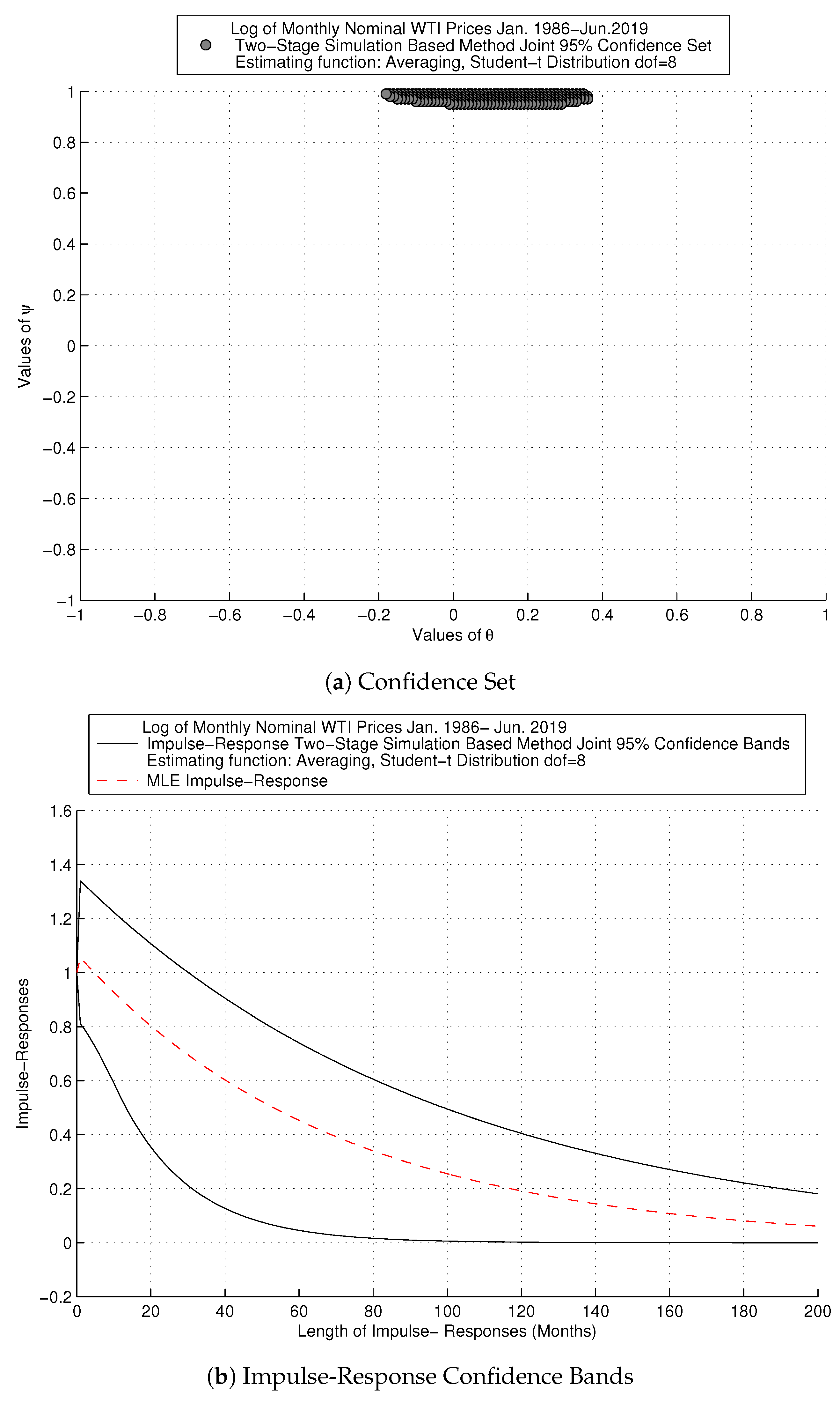
We focus on the framework with the averaging objective function, which refutes root cancelation for the price series. This result reinforces the usefulness of our combined strategy. Figure 2 focuses on the fatter tails calibration and the averaging objective function for the monthly nominal frequency and contains two diagrams: (i) joint confidence set and (ii) impulse-response confidence bands. Additionally, the second diagram displays the MLE impulse-response function, to illustrate that it can be misleading, since it is within our confidence bands. The confidence set obtained with our method in Figure 2a is sharp and supports the ARMA parametrization. Although the projections of the MA parameter contain zero, the MA root ranges from −0.18 to 0.36. The AR parameter takes values between 0.95 and 0.99. As a result, our impulse-response confidence bands in Figure 2b show a persistent effect of the shock on prices, which takes above a decade or so to die down.
We refute the ARMA (1,1) on weekly nominal returns, with both the Gaussian and the Student-t distributions, when combined with the OLS estimation of forward and backward-looking components as auxiliary function. This means that the model is not complex enough at this particular frequency. At the monthly nominal frequency, we also obtain an empty confidence set if the Gaussian distribution is combined with the same auxiliary function. In contrast, the model with the fatter tails calibration is never rejected at the monthly frequency. Non-empty confidence sets, obtained with both distributions at the monthly frequency are closed (one set), or disjoint (with two and three subsets) and exhibit shapes that are sharp and tight around root cancelation. Confidence sets are informative, since a large area of the parameter space is refuted. However, we cannot refute root cancelation, even with fatter tails.
Figure 3 shows results with the fatter tails calibration and the averaging method for the monthly nominal frequency of returns, following the same order as in the previous figure. Figure 3a exhibits the confidence set, which is sharp around root cancelation. Resulting impulse-response confidence bands in Figure 3b indicate that there is no persistence of the shock on returns, due to the effect of root cancelation.
Collected together, our results support research at the frequency typically used in macro analysis for oil series, with an ARMA in levels, including the Gaussian shock hypothesis. Thus, we find that shocks to oil prices are permanent, taking about a decade or so to die down. Confidence sets obtained with oil returns are quite sharp around root cancellation, which affects predictability at the frequencies examined. In addition, the ARMA specification is refuted at the weekly frequency of returns, which suggests that alternative specifications allowing for e.g., conditional heteroskedasticity and skewness are interesting research paths, on frequencies more relevant to finance than macro applications.
7. Conclusions
Our framework delivers simultaneous impulse-response confidence bands for ARMA (1,1) processes by combining Indirect Inference, MC test methods and confidence sets projections. We treat proposed objective functions as test statistics, which we invert through a two-stage simulation to obtain joint confidence sets for the parameters. Invariance principles are proposed to ensure finite sample exactness in general nuisance parameter dependent settings. In contrast to MLE-based tests, our proposed methods achieve size control and good power, irrespective of how close the parameters are to the unit root boundary, or whether root cancelation is present.
We investigate the persistence of shocks on oil prices and returns of the West Texas Intermediate (WTI) benchmark via projected impulse-response confidence bands. The main advantage of our method is the possibility of remaining agnostic with respect to the process followed by these series. It is noteworthy that resulting impulse-response confidence bands seem well identified. Our results support a persistent ARMA model in levels. In contrast, confidence sets for monthly returns are tightly concentrated on the root cancellation line. ARMA with or without fat tails is rejected for the weekly return series. This noteworthy result reinforces the usefulness of confidence set methods that allow for empty outcomes. Lastly, our findings support the applicability of impulse-responses obtained from asymmetric and heavy tailed distributions, which leaves the door open for further research, in particular with asymmetric distributions.
Author Contributions
The authors contributed equally to this work. All authors have read and agreed to the published version of the manuscript.
Funding
This work was supported by the Social Sciences and Humanities Research Council of Canada and the Fonds de recherche sur la société et la culture (Québec).
Conflicts of Interest
The authors declare no conflict of interest.
References
- Alquist, Ron, and Lutz Kilian. 2010. What do We Learn From the Price of Crude Oil Futures? Journal of Applied Econometrics 25: 539–73. [Google Scholar] [CrossRef] [Green Version]
- Alquist, Ron, Lutz Kilian, and Robert J. Vigfusson. 2013. Forecasting the Price of Oil. In Handbook of Economic Forecasting. Edited by Graham Elliott and Allan Timmermann. Amsterdam: Elsevier B.V., vol. 2, Part A. pp. 427–507. [Google Scholar]
- Andrews, Donald W. K., and Patrik Guggenberger. 2010. Asymptotic Size and a Problem with Subsampling and With the m out of n Bootstrap. Econometric Theory 26: 426–68. [Google Scholar] [CrossRef]
- Andrews, Donald W. K., and Xu Cheng. 2012. Estimation and Inference with Weak, Semi-Strong and Strong-Identification. Econometrica 80: 2153–11. [Google Scholar] [CrossRef] [Green Version]
- Andrews, Isaiah, and Anna Mikusheva. 2014. Weak Identification in Maximum Likelihood: A Question of Information. American Economics Review 104: 195–99. [Google Scholar] [CrossRef] [Green Version]
- Andrews, Isaiah, and Anna Mikusheva. 2015. Maximum Likelihood Inference in Weakly Identified Dynamic Stochastic General Equilibrium Models. Quantitative Economics 1: 123–52. [Google Scholar] [CrossRef] [Green Version]
- Ansley, Craig F., and Paul Newbold. 1980. Finite Sample Properties of Estimators for Auto-regressive Moving Average Processes. Journal of Econometrics 13: 159–84. [Google Scholar] [CrossRef]
- Ariel, Robert A. 1987. A Monthly Effect in Stock Returns. Journal of Financial Economics 18: 161–74. [Google Scholar] [CrossRef] [Green Version]
- Atkeson, Andrew, and Patrick J. Kehoe. 1999. Models of Energy Use: Putty-Putty versus Putty-Clay. American Economic Review 89: 1028–43. [Google Scholar] [CrossRef] [Green Version]
- Baumeister, Christiane, and Lutz Kilian. 2012. Real-Time Forecasts of the Real Price of Oil. Journal of Business & Economic Statistics 30: 326–36. [Google Scholar]
- Baumeister, Christiane, and Lutz Kilian. 2014a. Real-Time Analysis of Oil Price Risks Using Forecast Scenarios. IMF Economic Review 62: 120–45. [Google Scholar] [CrossRef] [Green Version]
- Baumeister, Christiane, and Lutz Kilian. 2014b. What Central Bankers Need to Know About Forecasting Oil Prices. International Economic Review 55: 869–89. [Google Scholar] [CrossRef] [Green Version]
- Baumeister, Christiane, Lutz Kilian, and Thomas K. Lee. 2014. Are There Gains from Pooling Real-Time Oil Price Forecasts? Energy Economics 46: 533–43. [Google Scholar] [CrossRef] [Green Version]
- Baumeister, Christiane, and Lutz Kilian. 2015. Forecasting the Real Price of Oil in a Changing World: A Forecast Combination Approach. Journal of Business and Economics Statistics 33: 338–51. [Google Scholar] [CrossRef] [Green Version]
- Baumeister, Christiane, Pierre Guérin, and Lutz Kilian. 2015. Do High-Frequency Financial Data Help Forecast Oil Prices? The MIDAS Touch at Work. International Journal of Forecasting 31: 238–52. [Google Scholar] [CrossRef] [Green Version]
- Beaulieu, Marie-Claude, Jean-Marie Dufour, and Lynda Khalaf. 2007. Multivariate Tests of Mean-Variance Efficiency with Possibly Non-Gaussian Errors: An Exact Simulation-Based Approach. Journal of Business and Economic Statistics 25: 398–410. [Google Scholar] [CrossRef]
- Beaulieu, Marie-Claude, Jean-Marie Dufour, and Lynda Khalaf. 2013. Identification-Robust Estimation and Testing of the Zero-Beta CAPM. Review of Economic Studies 80: 892–924. [Google Scholar] [CrossRef] [Green Version]
- Beaulieu, Marie-Claude, Jean-Marie Dufour, and Lynda Khalaf. 2014. Exact Confidence Set Estimation and Goodness of Fit Test Methods for Asymmetric Heavy Tailed Stable Distributions. Journal of Econometrics 181: 3–14. [Google Scholar] [CrossRef] [Green Version]
- Bernard, Jean-Thomas, Jean-Marie Dufour, Lynda Khalaf, and Maral Kichian. 2012. An Identification- Robust Test for Time-Varying Parameters in the Dynamics of Energy Prices. Journal of Applied Econometrics 27: 603–24. [Google Scholar] [CrossRef] [Green Version]
- Billio, Monica, and Alain Monfort. 2003. Kernel-Based Indirect Inference. Journal of Financial Econometrics 3: 297–326. [Google Scholar] [CrossRef]
- Calvet, Laurent E., and Veronika Czellar. 2015. Through the Looking Glass: Indirect Inference via Simple Equilibria. Journal of Econometrics 185: 343–58. [Google Scholar] [CrossRef]
- Calzolari, Giorgio, Gabriele Fiorentini, and Enrique Sentana. 2004. Constrained Indirect Estimation. The Review of Economic Studies Limited 71: 945–73. [Google Scholar] [CrossRef]
- Charles, Amelié, and Olivier Darné. 2014. Volatility Persistence in Crude Oil Markets. Energy Policy 65: 729–42. [Google Scholar] [CrossRef] [Green Version]
- Chaudhuri, Saraswata, David T. Frazier, and Eric Renault. 2018. Indirect Inference with Endogenously Missing Exogenous Variables. Journal of Econometrics 205: 55–75. [Google Scholar] [CrossRef]
- Choi, Kyongwook, and Shawkat Hammoudeh. 2009. Long Memory in Oil and Refined Product Markets. The Energy Journal 30: 97–116. [Google Scholar] [CrossRef]
- Davis, Richard A., and William T. M. Dunsmuir. 1996. Maximum Likelihood Estimation for MA(1) processes with a Root on the Unit Circle. Econometric Theory 12: 1–20. [Google Scholar] [CrossRef]
- Davis, Richard A., and Li Song. 2011. Unit Roots in Moving Averages Beyond First Order. Annals of Statistics 39: 3062–91. [Google Scholar] [CrossRef] [Green Version]
- Dominicy, Yves, and David Veredas. 2013. The Method of Simulated Quantiles. Journal of Econometrics 172: 235–47. [Google Scholar] [CrossRef] [Green Version]
- Dufour, Jean-Marie, Lynda Khalaf, and Marie-Claude Beaulieu. 2003. Exact Skewness and Kurtosis Tests for Multivariate Normality and Goodness of Fit in Multivariate Regressions with Application to Asset Pricing Models. Oxford Bulletin of Economics and Statistics 65: 891–906. [Google Scholar] [CrossRef] [Green Version]
- Dufour, Jean-Marie, Lynda Khalaf, and Marie-Claude Beaulieu. 2010. Finite Sample Diagnostics in Multivariate Regressions with Applications to Asset Pricing Models. Journal of Applied Econometrics 25: 263–85. [Google Scholar] [CrossRef]
- Dufour, Jean-Marie, and Jeong-Ryeol Kurz-Kim. 2010. Exact Inference and Optimal Invariant Estimation for the Stability Parameter of Symmetric α-Stable Distributions. Journal of Empirical Finance 17: 180–94. [Google Scholar] [CrossRef]
- Dufour, Jean-Marie. 2006. Monte Carlo Tests with Nuisance Parameters: A General Approach to Finite-Sample Inference and Nonstandard Asymptotics in Econometrics. Journal of Econometrics 133: 443–78. [Google Scholar] [CrossRef] [Green Version]
- Dufour, Jean-Marie, and Denis Pelletier. 2014. Practical Methods for Modelling Weak VARMA Processes: Identification, Estimation and Specification with a Macroeconomic Application. Available online: https://pdfs.semanticscholar.org/0801/2dbed27e21f9a6f12ca5a50caa12e7425227.pdf (accessed on 2 July 2019). Working Paper.
- Dufour, Jean-Marie, and Olivier Torrès. 2000. Markovian Processes, Two-Sided Autoregressions and Exact Inference for Stationary and Nonstationary Autoregressive Processes. Journal of Econometrics 99: 255–89. [Google Scholar] [CrossRef] [Green Version]
- Dufour, Jean-Marie, and Pascale Valéry. 2006. On a Simple Two-Stage Closed-Form Estimator for a Stochastic Volatility in a General Linear Regression. In Volume 20 (Part A) of Advances in Econometrics: Econometric Analysis of Economic and Financial Time Series. Edited by Thomas B. Fomby and Dek Terrell. Oxford: Elsevier Science, pp. 259–88. [Google Scholar]
- Dufour, Jean-Marie, and Pascale Valéry. 2009. Exact and Assymptotic Test for Possibly Non-Regular Hypothesis on Stochastic Volatility Models. Journal of Econometrics 150: 193–206. [Google Scholar] [CrossRef] [Green Version]
- Dridi, Ramdan, Alain Guay, and Eric Renault. 2007. Indirect Inference and Calibration of Dynamic Stochastic General Equilibrium Models. Journal of Econometrics 136: 397–430. [Google Scholar] [CrossRef]
- Energy Information Administration (EIA). 2019. WTI Prices in U.S. Dollars per Barrel Jan.1986-Jun. Available online: eia.gov (accessed on 2 July 2019).
- Forneron, Jean-Jacques, and Senera Ng. 2018. The ABC of Simulation Estimation with Auxiliary Statistics. Journal of Econometrics 205: 112–39. [Google Scholar] [CrossRef] [Green Version]
- French, Kenneth R. 1980. Stocks Returns, and the Weekend Effect. Journal of Financial Economics 8: 55–69. [Google Scholar] [CrossRef]
- Fuleky, Peter, and Eric Zivot. 2014. Indirect Inference Based on the Score. Econometrics Journal 17: 383–93. [Google Scholar] [CrossRef] [Green Version]
- Galbraith, John W., and Victoria Zinde-Walsh. 1994. A Simple, Non-Iterative Estimator for Moving Average Models. Biometrika 81: 143–56. [Google Scholar] [CrossRef]
- Galbraith, John W., and Victoria Zinde-Walsh. 1997. On Some Simple, Autoregression-Based Estimation and Identification Techniques for ARMA Models. Biometrika 84: 685–96. [Google Scholar] [CrossRef]
- Gallant, A. Ronald, and George Tauchen. 1996. Which Moments to Match. Econometric Theory 12: 657–81. [Google Scholar] [CrossRef]
- Genton, Marc G., and Elvezio Ronchetti. 2003. Robust Indirect Inference. Journal of the American Statistical Association 98: 67–76. [Google Scholar]
- Ghysels, Eric, Lynda Khalaf, and Cosmé Vodounou. 2003. Simulation Based Inference in Moving Average Models. Annales D’Economie et Statistique 69: 85–99. [Google Scholar] [CrossRef] [Green Version]
- Gil-Alana, Luis A., and Rangan Gupta. 2014. Persistence, and Cycles in Historical Oil Price Data. Energy Economics 45: 511–16. [Google Scholar] [CrossRef] [Green Version]
- Gorodnichenko, Yuriy, Anna Mikusheva, and Serena Ng. 2012. Estimators for Persistent, and Possibly Non-Stationary Data with Classical Properties. Econometric Theory 28: 1003–36. [Google Scholar] [CrossRef] [Green Version]
- Gospodinov, Nikolay. 2002. Bootstrap Based Inference in Models with a Nearly Noninvertible Moving Average Component. Journal of Business and Economic Statistics 20: 254–268. [Google Scholar] [CrossRef]
- Gospodinov, Nikolay, and Serena Ng. 2015. Minimum Distance Estimation of Possibly Non-Invertible Moving Average Models. Journal of Business and Economic Statistics 33: 403–17. [Google Scholar] [CrossRef] [Green Version]
- Gouriéroux, Christian, Alain Monfort, and Eric Renault. 1993. Indirect Inference. Journal of Applied Econometrics 8: S85–118. [Google Scholar] [CrossRef]
- Gouriéroux, Christian, and Alain Monfort. 1996. Simulation-Based Econometric Methods, Core Lectures. Oxford: Oxford University Press. [Google Scholar]
- Gouriéroux, Christian, Peter C. B. Phillips, and Jun Yu. 2010. Indirect Inference for Dynamic Panel Models. Journal of Econometrics 157: 68–77. [Google Scholar] [CrossRef]
- Guerron-Quintana, Pablo, Atsushi Inoue, and Lutz Kilian. 2017. Impulse response matching estimators for DSGE models. Journal of Econometrics 196: 144–55. [Google Scholar] [CrossRef] [Green Version]
- Guay, Alain, and Olivier Scaillet. 2003. Indirect Inference, Nuisance Parameter, and Threshold Moving Average Models. Journal of Business and Economic Statistics 21: 122–32. [Google Scholar] [CrossRef] [Green Version]
- Hamilton, James D. 1983. Oil, and the Macroeconomy since World War II. Journal of Political Economy 91: 228–48. [Google Scholar] [CrossRef]
- Hamilton, James D. 1996. This is What Happened to the Oil Price-Macroeconomy Relationship. Journal of Monetary Economics 38: 215–20. [Google Scholar] [CrossRef]
- Hamilton, James D. 2003. What Is an Oil Shock? Journal of Econometrics 113: 363–98. [Google Scholar] [CrossRef]
- Hamilton, James D. 2009. Understanding Crude Oil Prices. The Energy Journal 30: 179–205. [Google Scholar] [CrossRef] [Green Version]
- Hamilton, James D. 2011. Nonlinearities, and the Macroeconomic Effects of Oil Prices. Macroeconomic Dynamics 15: 364–78. [Google Scholar] [CrossRef] [Green Version]
- Hannan, Edward J., and Jorma Rissanen. 1982. Recursive Estimation of Mixed Autoregressive-Moving-Average Order. Biometrika 69: 81–94. [Google Scholar] [CrossRef]
- Hansen, Bruce E. 1999. The Grid Bootstrap, and the Autoregressive Model. Review of Economics, and Statistics 81: 594–607. [Google Scholar] [CrossRef]
- Harvey, Andrew C. 1981. Time Series Models. London: Philip Allan. [Google Scholar]
- Inoue, Atsushi, and Lutz Kilian. 2013. Inference on Impulse Response Functions in Structural VAR Models. Journal of Econometrics 177: 1–13. [Google Scholar] [CrossRef] [Green Version]
- Inoue, Atsushi, and Lutz Kilian. 2016. Joint Confidence Sets for Structural Impulse Responses. Journal of Econometrics 192: 421–32. [Google Scholar] [CrossRef] [Green Version]
- Jordà, Òscar. 2009. Simultaneous Confidence Regions for Impulse Responses. The Review of Economics, and Statistics 91: 629–47. [Google Scholar] [CrossRef]
- Jordà, Òscar, and Massimiliano Marcellino. 2010. Path Forecast Evaluation. Journal of Applied Econometrics 25: 635–62. [Google Scholar] [CrossRef] [Green Version]
- Jordà, Òscar, and Sharon Kozicki. 2011. Estimation, and Inference by the Method of Projection Minimum Distance: An Application to the New Keynesian Hybrid Phillips Curve. International Economic Review 52: 461–87. [Google Scholar] [CrossRef]
- Jordà, Òscar, Malte Knüppel, and Massimiliano Marcellino. 2013. Empirical Simultaneous Confidence Regions for Path-Forecasts. International Journal of Forecasting 29: 456–68. [Google Scholar] [CrossRef]
- Khalaf, Lynda, and Charles J. Saunders. 2019. Monte Carlo Two-Stage Indirect Inference (2SIF) for Autoregressive Panels. Forthcoming: The Journal of Econometrics. [Google Scholar]
- Kilian, Lutz. 2008a. A Comparison of the Effects of Exogenous Oil Supply Shocks on Output, and Inflation in the G7 Countries. Journal of the European Economic Association 6: 78–121. [Google Scholar] [CrossRef] [Green Version]
- Kilian, Lutz. 2008b. The Economic Effects of Energy Price Shocks. Journal of Economic Literature 46: 871–909. [Google Scholar] [CrossRef] [Green Version]
- Kilian, Lutz. 2008c. Exogenous Oil Supply Shocks: How Big Are They, and How Much Do They Matter for the U.S. Economy? Review of Economics, and Statistics 90: 216–40. [Google Scholar] [CrossRef]
- Kilian, Lutz. 2009. Not All Oil Price Shocks Are Alike: Disentangling Demand, and Supply Shocks in the Crude Oil Market. American Economic Review 99: 1053–69. [Google Scholar] [CrossRef] [Green Version]
- Kilian, Lutz. 2014. Oil Price Shocks: Causes, and Consequences. Annual Review of Resource Economics 6: 133–54. [Google Scholar] [CrossRef] [Green Version]
- Kilian, Lutz, and Robert J. Vigfusson. 2017. The Role of Oil Price Shocks in Causing U.S. Recessions. Journal of Money, Credit, and Banking 49: 1747–76. [Google Scholar] [CrossRef] [Green Version]
- Leduc, Sylvain, and Keith Sill. 2004. A Quantitative Analysis of Oil Price Shocks, Systematic Monetary Policy, and Economic Downturns. Journal of Monetary Economics 51: 781–808. [Google Scholar] [CrossRef] [Green Version]
- Lee, Junsoo, John A. List, and Mark C. Strazicich. 2006. Non-Renewable Resource Prices: Deterministic or Stochastic Trends? Journal of Environmental Economic Management 3: 354–70. [Google Scholar] [CrossRef] [Green Version]
- Li, Tong. 2010. Indirect Inference in Structural Econometric Models. Journal of Econometrics 157: 120–28. [Google Scholar] [CrossRef]
- Lubik, Thomas A., and Frank Schorfheide. 2003. Computing Sunspot Equilibria in Linear Rational Expectations Models. Journal of Economic Dynamics & Control 28: 273–85. [Google Scholar]
- Lubik, Thomas A., and Frank Schorfheide. 2004. Testing for Indeterminancy: An Application to U.S. Monetary Policy. The American Economic Review 94: 190–217. [Google Scholar] [CrossRef] [Green Version]
- Lütkepohl, Helmut, Anna Staszewska-Bystrova, and Peter Winker. 2015. Comparison of Methods for Constructing Joint Confidence Bands for Impulse Response Functions. International Journal of Forecasting 31: 782–98. [Google Scholar] [CrossRef] [Green Version]
- Mikusheva, Anna. 2007. Uniform Inference in Autoregressive Models. Econometrica 75: 1411–52. [Google Scholar] [CrossRef]
- Mikusheva, Anna. 2012. One-Dimensional Inference in Autoregressive Models with the Potential Presence of a Unit Root. Econometrica 80: 173–212. [Google Scholar]
- Mikusheva, Anna. 2014. Second Order Expansion of the t-statistic in AR(1) Models. Econometric Theory 31: 426–48. [Google Scholar] [CrossRef]
- Montiel Olea, José Luis, and Mikkel Plagborg-Møller. 2019. Simultaneous Confidence Bands: Theory, Implementation, and an Application to SVARs. Journal of Applied Econometrics 34: 1–17. [Google Scholar] [CrossRef] [Green Version]
- Nelson, Charles R., and Richard Startz. 2007. The Zero-information-limit Condition, and Spurious Inference in Weakly-identified Models. Journal of Econometrics 138: 47–62. [Google Scholar] [CrossRef]
- Phillips, Peter C. B. 2014. On Confidence Intervals for Autoregressive Roots, and Predictive Rgressions. Econometrica 82: 1177–95. [Google Scholar]
- Pindyck, Robert S. 1999. The Long Run Eolution of Energy Prices. The Energy Journal 20: 1–27. [Google Scholar] [CrossRef] [Green Version]
- Pindyck, Robert S. 2004. Volatility, and commodity price dynamics. Journal of Futures Markets 24: 1029–47. [Google Scholar] [CrossRef] [Green Version]
- Robins, James M., Aad van der Vaart, and Valérie Ventura. 2000. Asymptotic Distribution of P Values in Composite Null Models. Journal of the American Statistical Association 95: 1143–56. [Google Scholar]
- Ronchetti, Elvezio, and Fabio Trojani. 2001. Robust Inference with GMM Estimators. Journal of Econometrics 101: 37–69. [Google Scholar] [CrossRef] [Green Version]
- Sargan, John D., and Alok Bhargava. 1983. Maximum Likelihood Estimation of Regression Models with First Order Moving Average Errors when the Root Lies on the Unit Circle. Econometrica 51: 799–820. [Google Scholar] [CrossRef]
- Sims, Christopher A. 2001. Solving Linear Rational Expectations Models. Computational Economics 20: 1–20. [Google Scholar] [CrossRef]
- Smith, Anthony A., Jr. 1993. Estimating Nonlinear Time Series Models Using Simulated Vector Autoregressions. Journal of Applied Econometrics 8: S63–84. [Google Scholar] [CrossRef] [Green Version]
- Staszewska-Bystrova, Anna. 2007. Representing Uncertainty About Impulse Response Paths: The Use of Heuristic Optimization Methods. Computational Statistics, and Data Analysis 52: 121–32. [Google Scholar] [CrossRef]
- Staszewska-Bystrova, Anna. 2011. Bootstrap Prediction Bands for Forecast Paths from Vector Autoregressive Models. Journal of Forecasting 30: 721–35. [Google Scholar] [CrossRef]
- Staszewska-Bystrova, Anna. 2013. Modified Scheffé’s Prediction Bands. Journal of Economics, and Statistics 233: 680–90. [Google Scholar] [CrossRef]
- Staszewska-Bystrova, Anna, and Peter Winker. 2013. Constructing Narrowest Pathwise Bootstrap Prediction Bands Using Threshold Accepting. International Journal of Forecasting 29: 221–33. [Google Scholar] [CrossRef]
- Stock, James H. 1991. Confidence Intervals for the Largest Autoregressive Root in Macroeconomic Time Series. Journal of Monetary Economics 28: 435–59. [Google Scholar] [CrossRef]
- Stock, James H., and Mark W. Watson. 1993. A Simple Estimator of Cointegrating Vectors in Higher Order Integrated Systems. Econometrica 61: 783–820. [Google Scholar] [CrossRef]
- US. Bureau of Labor Statistics. 2019. Consumer Price Index for All Urban Consumers: All Items [CPIAUCSL], Index 1982–84=100, retrieved from the Federal Reserve Bank of St. Louis, Economic Data (FRED). Available online: https://fred.stlouisfed.org/series/CPIAUCSL/ (accessed on 5 July 2019).
| 1. | See, for example, Robins et al. (2000); Ronchetti and Trojani (2001); Calzolari et al. (2004); Dridi et al. (2007); Gouriéroux et al. (2010); Li (2010); Dominicy and Veredas (2013); Fuleky and Zivot (2014); Calvet and Czellar (2015); Chaudhuri et al. (2018) and Forneron and Ng (2018). |
| 2. | On simultaneous inference in related contexts see e.g., Jorda (2009); Jorda and Marcellino (2010); Jorda et al. (2013) on simultaneous path forecasts, and recently Montiel et al. (2019). |
| 3. | Throughout this document, size and coverage are used interchangeably; see Andrews and Cheng (2012). |
| 4. | In this regard, our work relates to Dufour and Valéry (2006, 2009) in stochastic volatility models, Dufour and Kurz-Kim (2010) and Beaulieu et al. (2007, 2013, 2014) in models with fat-tailed fundamentals. |
| 5. | |
| 6. | Alternatively, the data can be burned in to induce stationarity. Extensions to the mean-non stationarity framework as in Khalaf and Saunders (2019) is a worthy research direction. |
| 7. | Useful insight beyond the ARMA (1,1) on minimum dimension is found in the literature, in particular, Galbraith and Zinde-Walsh (1997) and more recently Gospodinov and Ng (2015). |
| 8. | This is noteworthy in view of the above cited problems discussed in the literature. |
| 9. | |
| 10. | Lütkepohl et al. (2015) provide an overview and evaluation in terms of coverage of the available literature dedicated to impulse-responses for VAR models and propose a new approach based on adjustments to the Bonferroni bands. |
| 11. | Alquist et al. (2013) explain that after mid-1980, due to the U.S. deregulation, the co-movement between the U.S. oil price series, including WTI, refiners acquisition cost for domestically produced oil and for imported crude oil, became stronger. This means that we can take the WIT, since results obtained with other series are expected to be similar due to the high correlation between the various U.S. oil price series. |
| 12. | At the time the series is retrieved, the latest available monthly value corresponds to May, 2019. |
| 13. | The U.S. subprime mortgage crisis triggered an international financial crisis in 2008. According to the U.S. National Bureau of Economics Research (NBER), the U.S. recession is identified in terms of peaks and troughs from the last quarter of 2007 to the second quarter of 2009. |
Figure 1.
West Texas Intermediate (WTI). Note: WTI prices escalated up to the highest peak during the month of July in 2008, when the price reached US$145 per barrel. Then, the effect of the financial crisis and Great Recession caused a price drop to US$30.28 in December of the same year.13 After 2014, WTI prices plummeted during the following three years, down to US$26.68 in January, 2016, mainly due to the effect of supply strategies, the surprising growth of U.S. shale oil production and by a slower-than-expected global growth, among others. The behaviour of WTI prices afterwards is associated with geopolitical risks and growth expectations for the U.S. and Chinese economies.

Figure 2.
SIM Method: Log of Monthly Nominal West Texas Intermediate (WTI) Prices.

Figure 3.
SIM Method: Monthly Nominal WTI Returns.


Table 1.
Data generated process (DGP) with .
| SIZE | ||||
|---|---|---|---|---|
| SIM Method | Gaussian MA | Student-t (df = 5) MA | ||
| OLS-Long AR | Simplified | OLS-Long AR | Simplified | |
| T = 50 | 0.046 | 0.040 | 0.043 | 0.038 |
| T = 100 | 0.054 | 0.055 | 0.047 | 0.042 |
| T = 200 | 0.046 | 0.049 | 0.053 | 0.039 |
| MLE | Gaussian MA | Student-t (df = 5) MA | ||
| T = 50 | 0.096 | 0.099 | ||
| T = 100 | 0.054 | 0.062 | ||
| T = 200 | 0.057 | 0.049 | ||
| POWER [SIM Method] | ||||
| T = 50 | Gaussian MA | Student-t (df = 5) MA | ||
| Tested Value | OLS-Long AR | Simplified | OLS-Long AR | Simplified |
| {0.00} | 0.717 | 0.861 | 0.720 | 0.865 |
| {0.30} | 0.322 | 0.364 | 0.302 | 0.370 |
| {0.85} | 0.276 | 0.225 | 0.266 | 0.211 |
| {0.90} | 0.368 | 0.286 | 0.371 | 0.267 |
| {0.96} | 0.436 | 0.324 | 0.430 | 0.302 |
| {0.99} | 0.442 | 0.334 | 0.442 | 0.309 |
| T = 100 | Gaussian MA | Student-t (df = 5) MA | ||
| Tested Value | OLS-Long AR | Simplified | OLS-Long AR | Simplified |
| {0.00} | 0.988 | 0.994 | 0.989 | 0.995 |
| {0.30} | 0.628 | 0.699 | 0.634 | 0.703 |
| {0.85} | 0.611 | 0.476 | 0.623 | 0.470 |
| {0.90} | 0.721 | 0.569 | 0.729 | 0.558 |
| {0.96} | 0.785 | 0.634 | 0.796 | 0.610 |
| {0.99} | 0.790 | 0.640 | 0.806 | 0.618 |
| T = 200 | Gaussian MA | Student-t (df = 5) MA | ||
| Tested Value | OLS-Long AR | Simplified | OLS-Long AR | Simplified |
| {0.00} | 1.000 | 1.000 | 1.000 | 1.000 |
| {0.30} | 0.926 | 0.935 | 0.934 | 0.942 |
| {0.85} | 0.910 | 0.786 | 0.910 | 0.779 |
| {0.90} | 0.960 | 0.869 | 0.967 | 0.862 |
| {0.96} | 0.978 | 0.914 | 0.983 | 0.908 |
| {0.99} | 0.980 | 0.919 | 0.984 | 0.912 |
Note: Numbers reported are empirical rejections for the hypothesis . Size is measured with and other choices for are reported as tested values in the power tables.
Table 2.
Data generated process (DGP) with .
| SIZE | ||||
|---|---|---|---|---|
| SIM Method | Gaussian MA | Student-t (df = 5) MA | ||
| OLS-Long AR | Simplified | OLS-Long AR | Simplified | |
| T = 50 | 0.052 | 0.045 | 0.048 | 0.041 |
| T = 100 | 0.054 | 0.053 | 0.045 | 0.038 |
| T = 200 | 0.039 | 0.042 | 0.039 | 0.042 |
| MLE | Gaussian MA | Student-t (df = 5) MA | ||
| T = 50 | 0.167 | 0.156 | ||
| T = 100 | 0.294 | 0.229 | ||
| T = 200 | 0.429 | 0.347 | ||
| POWER [SIM Method] | ||||
| T = 50 | Gaussian MA | Student-t (df = 5) MA | ||
| Tested Value | OLS-Long AR | Simplified | OLS-Long AR | Simplified |
| {0.00} | 0.998 | 0.993 | 0.998 | 0.993 |
| {0.30} | 0.948 | 0.854 | 0.961 | 0.842 |
| {0.60} | 0.594 | 0.363 | 0.573 | 0.353 |
| {0.85} | 0.095 | 0.073 | 0.091 | 0.061 |
| {0.90} | 0.061 | 0.054 | 0.059 | 0.049 |
| {0.96} | 0.057 | 0.045 | 0.051 | 0.041 |
| T = 100 | Gaussian MA | Student-t (df = 5) MA | ||
| Tested Value | OLS-Long AR | Simplified | OLS-Long AR | Simplified |
| {0.00} | 1.000 | 1.000 | 1.000 | 1.000 |
| {0.30} | 1.000 | 0.990 | 1.000 | 0.992 |
| {0.60} | 0.918 | 0.676 | 0.916 | 0.690 |
| {0.85} | 0.141 | 0.094 | 0.130 | 0.078 |
| {0.90} | 0.087 | 0.060 | 0.071 | 0.059 |
| {0.96} | 0.059 | 0.053 | 0.045 | 0.040 |
| T = 200 | Gaussian MA | Student-t (df = 5) MA | ||
| Tested Value | OLS-Long AR | Simplified | OLS-Long AR | Simplified |
| {0.00} | 1.000 | 1.000 | 1.000 | 1.000 |
| {0.30} | 1.000 | 1.000 | 1.000 | 1.000 |
| {0.60} | 0.996 | 0.922 | 0.996 | 0.928 |
| {0.85} | 0.204 | 0.099 | 0.196 | 0.124 |
| {0.90} | 0.084 | 0.050 | 0.079 | 0.063 |
| {0.96} | 0.042 | 0.039 | 0.043 | 0.040 |
Note: Numbers reported are empirical rejections for the hypothesis . Size is measured with and other choices for are reported as tested values in the power tables.
Table 3.
Data generated process (DGP) with .
| SIZE | ||||||
|---|---|---|---|---|---|---|
| SIM Method | Gaussian ARMA | Student-t (df = 5) ARMA | ||||
| OLS-FBLC | OLS-Long AR | AutoCorr | OLS-FBLC | OLS-Long AR | AutoCorr | |
| T = 50 | 0.056 | 0.053 | 0.038 | 0.041 | 0.049 | 0.033 |
| T = 100 | 0.053 | 0.054 | 0.058 | 0.041 | 0.048 | 0.051 |
| T = 200 | 0.049 | 0.045 | 0.054 | 0.049 | 0.043 | 0.061 |
| MLE | Gaussian ARMA | Student-t (df = 5) ARMA | ||||
| MA | AR | Joint | MA | AR | Joint | |
| T = 50 | 0.470 | 0.454 | 0.523 | 0.446 | 0.401 | 0.500 |
| T = 100 | 0.432 | 0.417 | 0.482 | 0.404 | 0.392 | 0.457 |
| T = 200 | 0.414 | 0.414 | 0.470 | 0.370 | 0.371 | 0.445 |
| POWER [SIM Method] | ||||||
| T = 50 | Gaussian ARMA | Student-t (df = 5) ARMA | ||||
| Tested Pair | OLS-FBLC | OLS-Long AR | AutoCorr | OLS-FBLC | OLS-Long AR | AutoCorr |
| {0, 0.6} | 0.430 | 0.225 | 0.181 | 0.418 | 0.229 | 0.174 |
| {0.3, 0.2} | 0.806 | 0.728 | 0.858 | 0.796 | 0.740 | 0.866 |
| {0.3, 0.85} | 0.923 | 0.699 | 0.453 | 0.932 | 0.702 | 0.428 |
| {0.5, 0.5} | 0.956 | 0.866 | 0.981 | 0.958 | 0.858 | 0.986 |
| {0.6, 0} | 0.836 | 0.436 | 0.180 | 0.828 | 0.431 | 0.170 |
| {0.6, 0.85} | 0.985 | 0.878 | 0.880 | 0.992 | 0.884 | 0.880 |
| {0.85, 0.2} | 0.999 | 0.916 | 0.307 | 0.999 | 0.904 | 0.271 |
| {0.85, 0.6} | 1.000 | 0.955 | 0.568 | 1.000 | 0.961 | 0.557 |
| {0.96, 0.5} | 1.000 | 0.961 | 0.481 | 1.000 | 0.963 | 0.471 |
| {0.99, 0.99} | 1.000 | 0.980 | 0.997 | 1.000 | 0.979 | 0.998 |
| T = 100 | Gaussian ARMA | Student-t (df = 5) ARMA | ||||
| Tested Pair | OLS-FBLC | OLS-Long AR | AutoCorr | OLS-FBLC | OLS-Long AR | AutoCorr |
| {0, 0.6} | 0.797 | 0.695 | 0.500 | 0.793 | 0.700 | 0.493 |
| {0.3, 0.2} | 0.980 | 0.998 | 0.991 | 0.981 | 0.999 | 0.990 |
| {0.3, 0.85} | 0.996 | 0.995 | 0.875 | 0.996 | 0.994 | 0.870 |
| {0.5, 0.5} | 0.999 | 1.000 | 0.999 | 1.000 | 1.000 | 0.999 |
| {0.6, 0} | 0.983 | 0.901 | 0.509 | 0.989 | 0.899 | 0.502 |
| {0.6, 0.85} | 1.000 | 1.000 | 0.992 | 1.000 | 1.000 | 0.991 |
| {0.85, 0.2} | 1.000 | 1.000 | 0.727 | 1.000 | 0.999 | 0.727 |
| {0.85, 0.6} | 1.000 | 1.000 | 0.933 | 1.000 | 1.000 | 0.932 |
| {0.96, 0.5} | 1.000 | 1.000 | 0.901 | 1.000 | 1.000 | 0.894 |
| {0.99, 0.99} | 1.000 | 1.000 | 1.000 | 1.000 | 1.000 | 1.000 |
| T = 200 | Gaussian ARMA | Student-t (df = 5) ARMA | ||||
| Tested Pair | OLS-FBLC | OLS-Long AR | AutoCorr | OLS-FBLC | OLS-Long AR | AutoCorr |
| {0, 0.6} | 0.984 | 0.979 | 0.887 | 0.987 | 0.983 | 0.894 |
| {0.3, 0.2} | 0.999 | 1.000 | 1.000 | 0.999 | 1.000 | 1.000 |
| {0.3, 0.85} | 1.000 | 1.000 | 0.998 | 1.000 | 1.000 | 0.996 |
| {0.5, 0.5} | 1.000 | 1.000 | 1.000 | 1.000 | 1.000 | 1.000 |
| {0.6, 0} | 0.999 | 0.999 | 0.911 | 1.000 | 0.999 | 0.918 |
| {0.6, 0.85} | 1.000 | 1.000 | 1.000 | 1.000 | 1.000 | 1.000 |
| {0.85, 0.2} | 1.000 | 1.000 | 0.994 | 1.000 | 1.000 | 0.992 |
| {0.85, 0.6} | 1.000 | 1.000 | 1.000 | 1.000 | 1.000 | 0.999 |
| {0.96, 0.5} | 1.000 | 1.000 | 0.998 | 1.000 | 1.000 | 0.998 |
| {0.99, 0.99} | 1.000 | 1.000 | 1.000 | 1.000 | 1.000 | 1.000 |
Note: Numbers reported are empirical rejections for the hypothesis and . Size is measured with and . Other choices for and are reported as tested values in the power tables.
Table 4.
Data generated process (DGP) with .
| SIZE | ||||||
|---|---|---|---|---|---|---|
| SIM Method | Gaussian ARMA | Student-t (df = 5) ARMA | ||||
| OLS-FBLC | OLS-Long AR | AutoCorr | OLS-FBLC | OLS-Long AR | AutoCorr | |
| T = 50 | 0.044 | 0.041 | 0.052 | 0.049 | 0.038 | 0.049 |
| T = 100 | 0.049 | 0.041 | 0.053 | 0.049 | 0.035 | 0.048 |
| T = 200 | 0.052 | 0.058 | 0.051 | 0.048 | 0.046 | 0.043 |
| MLE | Gaussian ARMA | Student-t (df = 5) ARMA | ||||
| MA | AR | Joint | MA | AR | Joint | |
| T = 50 | 0.140 | 0.060 | 0.171 | 0.119 | 0.060 | 0.153 |
| T = 100 | 0.281 | 0.068 | 0.259 | 0.223 | 0.049 | 0.227 |
| T = 200 | 0.390 | 0.074 | 0.349 | 0.317 | 0.049 | 0.281 |
| POWER [SIM Method] | ||||||
| T = 50 | Gaussian ARMA | Student-t (df = 5) ARMA | ||||
| Tested Pair | OLS-FBLC | OLS-Long AR | AutoCorr | OLS-FBLC | OLS-Long AR | AutoCorr |
| {0, 0.6} | 0.922 | 1.000 | 0.915 | 0.921 | 1.000 | 0.914 |
| {0.3, 0.2} | 0.831 | 1.000 | 0.992 | 0.830 | 1.000 | 0.991 |
| {0.3, 0.85} | 0.609 | 0.979 | 0.331 | 0.615 | 0.985 | 0.332 |
| {0.5, 0.5} | 0.295 | 0.968 | 0.904 | 0.305 | 0.980 | 0.906 |
| {0.5, 0.96} | 0.285 | 0.778 | 0.046 | 0.290 | 0.794 | 0.046 |
| {0.6, 0} | 0.427 | 0.998 | 0.998 | 0.442 | 0.999 | 0.992 |
| {0.6, 0.85} | 0.131 | 0.653 | 0.317 | 0.131 | 0.663 | 0.308 |
| {0.85, 0.2} | 0.017 | 0.763 | 0.980 | 0.020 | 0.772 | 0.986 |
| {0.85, 0.6} | 0.023 | 0.304 | 0.815 | 0.024 | 0.293 | 0.825 |
| {0.96, 0.5} | 0.040 | 0.257 | 0.891 | 0.038 | 0.241 | 0.893 |
| T = 100 | Gaussian ARMA | Student-t (df = 5) ARMA | ||||
| Tested Pair | OLS-FBLC | OLS-Long AR | AutoCorr | OLS-FBLC | OLS-Long AR | AutoCorr |
| {0, 0.6} | 0.997 | 1.000 | 0.994 | 0.997 | 1.000 | 0.995 |
| {0.3, 0.2} | 0.980 | 1.000 | 1.000 | 0.984 | 1.000 | 1.000 |
| {0.3, 0.85} | 0.908 | 1.000 | 0.635 | 0.914 | 1.000 | 0.648 |
| {0.5, 0.5} | 0.690 | 1.000 | 0.993 | 0.701 | 1.000 | 0.994 |
| {0.5, 0.96} | 0.662 | 0.984 | 0.074 | 0.671 | 0.988 | 0.070 |
| {0.6, 0} | 0.826 | 1.000 | 1.000 | 0.824 | 1.000 | 1.000 |
| {0.6, 0.85} | 0.418 | 0.939 | 0.610 | 0.435 | 0.947 | 0.626 |
| {0.85, 0.2} | 0.036 | 0.983 | 1.000 | 0.042 | 0.984 | 1.000 |
| {0.85, 0.6} | 0.035 | 0.508 | 0.976 | 0.033 | 0.531 | 0.973 |
| {0.96, 0.5} | 0.039 | 0.453 | 0.991 | 0.048 | 0.444 | 0.994 |
| T = 200 | Gaussian ARMA | Student-t (df = 5) ARMA | ||||
| Tested Pair | OLS-FBLC | OLS-Long AR | AutoCorr | OLS-FBLC | OLS-Long AR | AutoCorr |
| {0, 0.6} | 1.000 | 1.000 | 1.000 | 1.000 | 1.000 | 1.000 |
| {0.3, 0.2} | 1.000 | 1.000 | 1.000 | 1.000 | 1.000 | 1.000 |
| {0.3, 0.85} | 0.991 | 1.000 | 0.922 | 0.992 | 1.000 | 0.921 |
| {0.5, 0.5} | 0.943 | 1.000 | 1.000 | 0.943 | 1.000 | 1.000 |
| {0.5, 0.96} | 0.932 | 1.000 | 0.157 | 0.935 | 1.000 | 0.163 |
| {0.6, 0} | 0.984 | 1.000 | 1.000 | 0.984 | 1.000 | 1.000 |
| {0.6, 0.85} | 0.778 | 0.998 | 0.911 | 0.780 | 0.999 | 0.910 |
| {0.85, 0.2} | 0.121 | 1.000 | 1.000 | 0.100 | 1.000 | 1.000 |
| {0.85, 0.6} | 0.052 | 0.840 | 1.000 | 0.034 | 0.833 | 0.999 |
| {0.96, 0.5} | 0.067 | 0.767 | 1.000 | 0.067 | 0.763 | 1.000 |
Note: Numbers reported are empirical rejections for the hypothesis and . Size is measured with and . Other choices for and are reported as tested values in the power tables.
Table 5.
Data generated process (DGP) with .
| POWER [SIM Method] | |||
|---|---|---|---|
| T = 100 | Gaussian ARMA | ||
| Tested Pair | OLS-FBLC | OLS-Long AR | AutoCorr |
| {0, 0.6} | 0.903 | 0.998 | 0.326 |
| {0.3, 0.2} | 0.978 | 0.999 | 0.974 |
| {0.3, 0.85} | 0.994 | 0.999 | 0.310 |
| {0.5, 0.5} | 0.998 | 1.000 | 0.275 |
| {0.5, 0.96} | 1.000 | 1.000 | 0.918 |
| {0.6, 0} | 0.998 | 0.999 | 0.993 |
| {0.6, 0.85} | 1.000 | 1.000 | 0.327 |
| {0.85, 0.2} | 1.000 | 1.000 | 0.862 |
| {0.85, 0.6} | 1.000 | 1.000 | 0.105 |
| {0.96, 0.5} | 1.000 | 1.000 | 0.231 |
| {0.99, 0.99} | 1.000 | 1.000 | 0.987 |
Table 6.
Data generated process (DGP) with .
| POWER [SIM Method] | |||
|---|---|---|---|
| T = 100 | Gaussian ARMA | ||
| Tested Pair | OLS-FBLC | OLS-Long AR | AutoCorr |
| {0, 0.6} | 0.635 | 0.931 | 0.962 |
| {0.3, 0.2} | 0.403 | 0.957 | 1.000 |
| {0.3, 0.85} | 0.171 | 0.198 | 0.233 |
| {0.5, 0.5} | 0.066 | 0.130 | 0.959 |
| {0.5, 0.96} | 0.105 | 0.117 | 0.103 |
| {0.6, 0} | 0.056 | 0.733 | 1.000 |
| {0.6, 0.85} | 0.289 | 0.227 | 0.208 |
| {0.85, 0.2} | 0.858 | 0.562 | 0.997 |
| {0.85, 0.6} | 0.930 | 0.814 | 0.898 |
| {0.96, 0.5} | 0.974 | 0.860 | 0.956 |
| {0.99, 0.99} | 0.981 | 0.969 | 0.282 |
Note: Numbers reported are empirical rejections for the hypothesis and . Various choices for and are reported as tested values in the power tables.
Table 7.
Summary of Statistics. (Demeaned series).
| Time Period | Sample | Obs. | Mean | Std. Dev. | Skewness | Kurtosis |
|---|---|---|---|---|---|---|
| Jan. 1986–June 2019 | Log of Weekly Nominal Prices | 1732 | −2.8881 × | 0.6582 | 0.6582 | 1.6844 |
| Jan.1986–June 2019 | Log of Monthly Nominal Prices | 402 | 5.0485 × | 0.6566 | 0.2541 | 1.6844 |
| Jan. 1986–May 2019 | Log of Monthly Real Prices | 401 | 9.5241 × | 0.8719 | 0.1165 | 1.5428 |
| Jan. 1986–June 2019 | Weekly Nominal Returns | 1731 | 4.7302 × | 0.05128 | −0.1449 | 5.9181 |
| Jan. 1986–June 2019 | Monthly Nominal Returns | 401 | 6.9216 × | 0.10253 | −0.35965 | 4.9748 |
| Jan. 1986–May 2019 | Monthly Real Returns | 400 | 2.2898 × | 0.10341 | −0.37958 | 5.0612 |
© 2020 by the authors. Licensee MDPI, Basel, Switzerland. This article is an open access article distributed under the terms and conditions of the Creative Commons Attribution (CC BY) license (http://creativecommons.org/licenses/by/4.0/).
Share and Cite
MDPI and ACS Style
Khalaf, L.; Peraza López, B. Simultaneous Indirect Inference, Impulse Responses and ARMA Models. Econometrics 2020, 8, 12. https://doi.org/10.3390/econometrics8020012
AMA Style
Khalaf L, Peraza López B. Simultaneous Indirect Inference, Impulse Responses and ARMA Models. Econometrics. 2020; 8(2):12. https://doi.org/10.3390/econometrics8020012
Chicago/Turabian StyleKhalaf, Lynda, and Beatriz Peraza López. 2020. "Simultaneous Indirect Inference, Impulse Responses and ARMA Models" Econometrics 8, no. 2: 12. https://doi.org/10.3390/econometrics8020012
Note that from the first issue of 2016, this journal uses article numbers instead of page numbers. See further details here.