
Machine Learning for Simulation of Urban Heat Island Dynamics Based on Large-Scale Meteorological Conditions


1
Research Computing Center, Lomonosov Moscow State University, 1/4 Leninskie Gory, Moscow 119234, Russia
2
Moscow Center for Fundamental and Applied Mathematics, 1 Leninskie Gory, Moscow 119991, Russia
3
Shirshov Institute of Oceanology, Russian Academy of Sciences, 36 Nakhimovskiy prospect, Moscow 117997, Russia
4
Moscow Institute of Physics and Technology, 9 Institutskiy per., Dolgoprudny 141701, Russia
5
Faculty of Geography, Lomonosov Moscow State University, 1 Leninskie Gory, Moscow 119991, Russia
*
Author to whom correspondence should be addressed.
Climate 2023, 11(10), 200; https://doi.org/10.3390/cli11100200
Submission received: 14 August 2023
/
Revised: 24 September 2023
/
Accepted: 27 September 2023
/
Published: 2 October 2023
(This article belongs to the Special Issue The Built Environment in a Changing Climate: Interactions, Challenges and Perspectives: Part II)
Abstract
:This study considers the problem of approximating the temporal dynamics of the urban-rural temperature difference (ΔT) in Moscow megacity using machine learning (ML) models and predictors characterizing large-scale weather conditions. We compare several ML models, including random forests, gradient boosting, support vectors, and multi-layer perceptrons. These models, trained on a 21-year (2001–2021) dataset, successfully capture the diurnal, synoptic-scale, and seasonal variations of the observed ΔT based on predictors derived from rural weather observations or ERA5 reanalysis. Evaluation scores are further improved when using both sources of predictors simultaneously and involving additional features characterizing their temporal dynamics (tendencies and moving averages). Boosting models and support vectors demonstrate the best quality, with RMSE of 0.7 K and R2 > 0.8 on average over 21 years. For three selected summer and winter months, the best ML models forced only by reanalysis outperform the comprehensive hydrodynamic mesoscale model COSMO, supplied by an urban canopy scheme with detailed city-descriptive parameters and forced by the same reanalysis. However, for a longer period (1977–2023), the ML models are not able to fully reproduce the observed trend of ΔT increase, confirming that this trend is largely (by 60–70%) driven by megacity growth. Feature importance assessment indicates the atmospheric boundary layer height as the most important control factor for the ΔT and highlights the relevance of temperature tendencies as additional predictors.
1. Introduction
Urban heat island (UHI), i.e., a temperature excess in the cities with respect to their rural or natural surroundings, is the most obvious and most studied feature of urban climate that appears due to land cover modifications and anthropogenic activity. Such temperature excess may exceed 10 K under favorable calm and clear weather conditions [1,2,3] and affects urban dwellers and ecosystems in different ways. The UHI increases heat stress for urban citizens and even heat-related mortality during heat waves [4,5], serves as one of the driving factors for urban-induced impacts on convective processes and related dangerous weather events, including intense precipitation and thunderstorms [6,7], and modifies phenology cycles [8,9]. Hence, accurate data on the UHI is important for various practical applications, from weather forecasting to urban environmental management and climate change adaptation.
Given the deficit of in situ meteorological data in cities, hydrodynamic mesoscale models of the atmosphere are nowadays one of the main tools for obtaining spatially and temporally detailed data on the UHI. Such models coupled to urban canopy parameterizations [10,11] with a grid spacing of a few kilometers to hundreds of meters are able to reproduce the majority of urban-induced meteorological effects [12] and are routinely used in numerical weather prediction [13,14], regional heat stress assessments [15,16] and refinements of the climate change scenarios [17,18] for urban areas. However, such models demand computing resources and require complex software and hardware infrastructure (data storage, input and output data processing, etc.). Typically, such models are run on supercomputers using hundreds to thousands of computational cores.
Alternatively, statistical models can be used to predict the UHI. These methods are easier to use and computationally cheap, but they are not physically based explicitly and require retuning for each city. Statistical models are often used to approximate urban-rural temperature differences, called UHI magnitude or UHI intensity, based on available observations and a set of predictors, and then to predict them for new points in time and/or space. Several studies used multiple linear regressions to model spatial patterns of the UHI based on landcover-dependent predictors such as building and road density, albedo, greenery, etc. [19,20,21]. Other studies propose a statistical approximation of the UHI magnitude at a fixed site and its temporal variations forced by diurnal and seasonal cycles as well as meteorological conditions. Statistical models in such studies are typically trained using long-term UHI observations and reanalysis-based predictors such as wind speed, cloud cover, and humidity, and are further forced by climate projections to predict future UHI changes [22,23,24] or by the same reanalysis data for a longer period in order to distinguish UHI changes under the influence of urban growth and climate change [25]. Theeuwes et al. (2017) [26] proposed a diagnostic equation both for temporal and spatial variations of the daily maximum UHI magnitude, where predictors for temporal variation include incoming shortwave radiation, diurnal temperature range, and wind speed.
A new stage in the development of statistical modeling of meteorological variables is associated with the rapid spread of modern methods of machine learning (ML), which are gaining increasing popularity in the geosciences. ML methods have already been used, e.g., for statistical modeling of the precipitation amounts [27,28], air temperature [29], wind speed [30,31,32], and aerosol concentrations [33], for forecasting of the sea wave height [34], and mapping of the sea surface height [35]. Not surprisingly, ML methods have already found their applications in urban meteorology, primarily for downscaling and data fusion with the ultimate goal of detailed temperature mapping in cities [36,37,38,39,40,41] and even for reconstruction of 3D temperature and velocity fields around buildings [42].
Despite the abundance of studies focused on the ML-based spatial modeling of the UHI and other urban climate anomalies, much fewer ML-based studies are focused on the temporal variability of such anomalies. A few examples include London’s climate reconstruction over 70 years using a generalized additive model [25] and the reconstruction of the evaporation time series for urban landscapes [43]. However, the issues of comparing different ML models and selecting the best predictors for the problem of statistical modeling of the temporal dynamics of urban climate anomalies remain unexplored.
Our study aims to conduct a deeper investigation of the possibilities and limitations of state-of-the-art ML models to approximate and predict the observed temporal dynamics of the UHI magnitude based on background meteorological variables. We use long-term meteorological observations available for the mid-latitude megacity of Moscow, Russia, to address the following research questions: (1) to what extent ML models are able to reproduce the UHI magnitude based on predictors characterizing background meteorological conditions; (2) what is the difference between state-of-the-art ML models in the performance of the UHI approximation; and (3) what are the most relevant predictors for the UHI magnitude. The presentation has the following structure: the next Section 2 describes the study area and meteorological data, provides a statement of the machine learning problem, and presents the specific ML models used in our study. Section 3 presents and discusses the results, including quantitative metrics of models’ performance and predictors’ importance. Section 4 highlights our conclusion and outlook.
2. Data and Methods
2.1. Study Area
Moscow is the biggest Russian and European monocentric urban agglomeration with a population of approximately 17 million people [44], including the population of Moscow city as a federal subject of Russia and surrounding satellite cities in Moscow Oblast federal subject. The actual area of the city (excluding the suburbs and undeveloped areas) is about 1000 km2. The city experienced intensive and almost linear population growth in the second half of the XX century as well as in the XXI century. Since the middle of the XX century, the population of Moscow as a federal subject of Russia has more than doubled and reached almost 13 million people in 2022 (Supplementary Figure S1). Population growth was accompanied by urban sprawl and an increase in building height and density.
Moscow has a temperate humid, moderately continental climate (Dfb in Köppen climate classification) with a mean annual temperature of 6.3 °C and mean June and January temperatures of 19.6 °C and −6.3 °C, respectively (values are given for VDNKh weather station, WMO ID 27612, that is typically used to characterize Moscow climate, for the 1991–2020 period). Due to the cold winters, Moscow is known as one of the world’s coldest megacities. The urban-induced meteorological phenomena of Moscow are easy to detect against the homogeneous surroundings and quasi-symmetric urban planning features, which makes the city a convenient site for urban climate research. The city experiences an intense UHI with an increasing magnitude trend over the last decades [45,46,47], with a present-day annual-mean UHI magnitude of 2 K peaking at more than 10 K during calm and clear nights [3,45,46].
2.2. Meteorological Data
Our study is based on long-term, regular observations at the weather stations in the Moscow region, operated by the Russian National Hydrometeorological Service (Roshydroment). In total, we use data from 10 weather stations (Figure 1a), including the Balchug weather station (WMO ID 27605) in the center of Moscow. It is located in a densely built area in the historical city center, less than 1 km from the Kremlin (Figure 1b,c). Long-term meteorological observations are also available for a few other stations within Moscow megacity [45,48], but they are located within heterogeneous surroundings or in urban parks, and only the Balchug weather station is located in a quasi-homogeneous built environment. The Balchug site experiences higher temperatures than other urban weather stations and represents a hotspot of the Moscow UHI [45,49,50]. In terms of the Local Climate Zones (LCZs) classification [51], Balchug weather station represents LCZ 2 “compact midrise”. To characterize the background conditions, we used the data for nine stations surrounding the city, namely Klin (WMO ID 27417), Dmitrov (WMO ID 27419), Pavlovsky Posad (WMO ID 27523), Novo-Jerusalim (WMO ID 27511), Naro-Fominsk (WMO ID 27611), Serpukhov (WMO ID 27618), Kolomna (WMO ID 27625), Maloyaroslavets (WMO ID 27606), and Aleksandrov (WMO ID 27428). These stations are further referred to as rural, though they may be affected by local anthropogenic effects due to their location close to smaller towns or within rural/suburban settlements.
The observational dataset was compiled from the archives of the All-Russia Research Institute of Hydrometeorological Information, the World Data Centre (http://meteo.ru/, accessed on 1 October 2023), the Hydrometeorological Research Center of the Russian Federation, and the Central Administration of Hydrological and Environmental Monitoring (http://www.ecomos.ru/, accessed on 1 October 2023).
We also use state-of-the-art global atmospheric reanalysis ERA5 produced by the European Center for mid-range weather forecasts (ECMWF) [52] as an alternative and/or supplementary to observations. Reanalysis data with its original grid spacing of 0.25° was derived from the Copernicus climate data store. The high quality of ERA5 reanalysis, noted in a large number of works, e.g., in [53,54,55], allows us to expect good quality in its reproduction of the large-scale atmospheric processes in the Moscow region. Yet, it is important to note that reanalysis does not take into account urban-induced climate features, including the UHI, due to its coarse resolution and absence of an urban parameterization in the ECMWF Integrated Forecasting System (IFS) atmospheric model used to produce ERA5 (such parameterization is currently under development and testing [56]).
2.3. Statement of the Machine Learning Problem
We aim to approximate the UHI dynamics in the center of Moscow on time scales ranging from hours to decades based on a set of predictors characterizing the large-scale meteorological regime over a background (mostly non-urban) area. Our target variable is UHI magnitude, defined as , where is the temperature measured in the center of Moscow at the Balchug weather station, for each moment of time is defined as the average temperature over nine selected rural weather stations. The same definition of the UHI magnitude is used in several previous urban climate studies for Moscow [46,49,50].
Two formulations of the ML problem are considered. In the first one, at the i-th time moment is approximated by a model based on instant values of the predictors … characterizing the large-scale meteorological conditions for the same moment:
The second formulation accounts for the delayed connections between and predictors by using the values of the latter for several time steps prior to the i-th time moment:
2.4. Predictors of the UHI Magnitude
Based on the theoretical knowledge about UHI control factors [57] and data availability, we selected several meteorological variables that may be relevant as predictors of the UHI magnitude. These variables are listed in Table 1. Air temperature, humidity, wind speed, and cloud cover fraction are available both from observations and reanalysis. The rest we take only from the reanalysis. Among them, several variables are observed as well, yet we do not include these observations because of data availability problems or methodological issues. For example, precipitation is observed two or four times per day instead of 8 times per day for other variables, while the reanalysis provides hourly data for all variables, including precipitation.
Since the problem statement assumes the use of the characteristics of a large-scale meteorological regime, predictor values are obtained by averaging the observed meteorological variables over nine selected background weather stations around Moscow (Figure 1). In the case of gaps for one or more stations, the averaging is carried out for the remaining ones. For reanalysis data, we perform areal averaging over a 3 × 3 grid cell set centered over Moscow. It is worth noting that the predictors derived both from observation and reanalysis are not necessarily highly correlated. The best agreement is found for rural temperature t2m, with a slight negative bias of 0.3 K and a correlation coefficient of almost 1. However, it is much worse for wind speed and cloudiness (Supplementary Table S1). Such differences may be due to a large number of factors. In any case, from a machine learning point of view, having a large number of uncorrelated predictors is good.
For the second approach (Equation (2)), we design additional features characterizing delayed connections between and meteorological predictors (hereafter called temporal features, or TFs). Firstly, we use the tendencies of each meteorological variable during 3, 6, and 12 h prior to the i-th time moment, defined for the k-th variable as . Secondly, we use left-side moving averages (MAs) with window widths of 3, 6, and 12 h, defined as and so on.
In addition, we use a so-called weather factor (WF) as a predictor for , an empirical function, of wind speed, cloud fraction and cloud type, as suggested in [58] and explained in more detail in [59]. We use a slightly simplified formulation based on 10-m wind speed (vel10m), total (tcc), and low (lcc) cloud fractions, which allows WF to be calculated without information about cloud type and is applicable both for observations and reanalysis.
We calculate WF independently based on observations and reanalysis but do not calculate its temporal features.
In addition to weather-dependent predictors, we consider the so-called astronomical predictors, i.e., diurnal and seasonal cycles. These factors include solar height, the day’s position in the seasonal cycle, and position in the diurnal cycle.
To compare the relevance of different predictors, we independently consider six sets of predictors (Table 2). Firstly, we analyze the opportunity to approximate UHI magnitude using different types of source data and consider sets of observation-based predictors (a), reanalysis-based predictors (b), and both types of predictors combined together (c). Secondly, we analyze the impact of temporal features by comparing approaches (1) and (2). Temporal features are calculated for all meteorological variables based on observations (2a), reanalysis (2b), or both (2c). Astronomical predictors are included in all sets.
To train and validate ML models, we use the dataset that includes target variable and abovementioned predictors over an almost 21-year period starting from 1 January 2001 to 31 August 2021 with 3-hourly temporal spacing, which gives 60,385 rows. The selection of such a period is determined by a tradeoff between dataset size and the homogeneity of the climatic conditions. After excluding rows with a missing value of the target variable or at least one predictor, 60,091 rows remain for combinations of predictors involving observations (1a, 1c, 2a, 2c), and 60,135 rows remain for the reanalysis-based datasets (1b, 2b).
Additionally, we use a dataset for a more than twice-longer period from 01.01.1977 to 31.08.2023 (almost 47 years) in order to evaluate model quality against the background of much larger climate change and urban growth [45,46]. During this longer period, the population of Moscow as an administrative unit has increased by 65%, from 7.8 million in 1977 to almost 13 million in 2022 (Supplementary Figure S1). In comparison, during the basic study period of 2001–2021, the population changed by 24%, from 10.2 to 12.6 million.
2.5. Machine Learning Models
The so-called “no free lunch theorem” [60,61] in its various forms establishes in general that, for an ML model, any elevated performance over one class of problems is offset by performance over another class. As a result, there are no ML models that would perform better than others in all possible classes of problems, given all reasonable measures of quality being assessed using all reasonable options of cross-validation. Rather, being averaged over a large set of problem classes, quality measures, and cross-validation approaches with several definitions of averaging, all algorithms have the same average off-training-set empirical risk level. Thus, there is no reliable way to presume one model’s superiority over others. Instead, one needs to try several promising methods in order to exploit the opportunity of choosing the best one. In this study, we explore the capabilities of six different ML models (see Table 3) in the problem of UHI magnitude approximation from large-scale predictors described above. Assessing multiple algorithms, we intend to cover the most promising models among a wide variety of ML methods that are capable of performing regression tasks on tabular data.
We employ ridge regression (RR) as a baseline statistical approach. RR is a linear model with ordinary least squares loss yet regularized by the sum of squared parameters of the model (a.k.a. L2 regularization). RR is a biased parameter estimator for the linear model, which is often used to address the issue of feature collinearity in multidimensional linear regression [62,63]. There are other regularizations that aim to overcome the issue of feature non-orthogonality, resulting in the Lasso model [64] in the case of L1 regularization (meaning the sum of absolute values of model parameters as an additive loss component) and ElasticNet exploiting the weighted sum of L2 and L2 regularization terms. Regarding this variety of regularization choices, in this study, we employ only the RR method, since we did not expect the linear model to deliver high quality compared to other machine learning approaches; thus, we only needed the level of baseline accuracy.
Among the more advanced statistical models, we compare the nonparametric random forests regression (RFR), gradient boosting regression (GBR), CatBoost regression (CBR), and support vector regression (SVR) models. We also use a regression model based on multilayer perceptron (MLPR), which is a fully connected class of feedforward artificial neural networks. We use the software implementation from the scikit-learn (version 0.24.2) Python library for all models except CBR, which is provided as an independent catboost (version 1.06) module.
Here, we outline the fundamentals of each model. RFR, GBR, and CBR are non-parametric ensemble models based upon the basic algorithms of decision trees (DT) [65,66,67]. DT is a popular ML model used for both classification and regression. They are tree-structured models where the leaves represent either class labels in cases of classification or a range of a real-valued target variable in cases of regression tasks and the branches (data subset splits) represent conjunctions of features that lead to those class labels. The main approach of decision trees is to generate an algorithm involving dataset splitting operations on the basis of rules generated within a greedy approach of optimal (maximum) reduction of the total empirical cost of the resulting regressor with each split. DT models are prone to overfitting [68], yet their expressive power is strongly dependent on hyperparameters, which include tree maximum depth (the maximum number of branches), among many others. In this study, we do not exploit DT as is, since they demonstrate this strong dependency of bias and variance on depth hyperparameter. However, we exploit ensembles of DT: Random Forests [69] and Gradient Boosting Machines (GBM) [70]. GBM is implemented in the form of the GBR algorithm in the scikit-learn package as well as CBR, an open-source boosting model developed by Yandex that performs exceptionally well on categorical datasets [71,72]. The main approach of GBM is to sequentially build an ensemble of weak algorithms, namely DT, characterized by low depth (also known as decision stumps). The ensemble is built in such a way that each DT is trained on the residuals of the previous ensemble. The most influential hyperparameter of all three ensemble models is the number of ensemble members (also known as estimators). This hyperparameter is mentioned in Table 3 as “n_estimators”, and we have performed the optimization regarding this option as described further.
Support vector machines [73] for Regression (SVR) [74] have emerged as a powerful tool for solving regression problems since 1996. SVR exploits the geometric interpretation of feature space and the power of kernel functions employed in kernel-equipped SVR. The main advantage of SVR is that there are almost no strongly influencing hyperparameters except the kernel function, which is hard to choose on the basis of prior knowledge. In our study, we employed the SVR model, for the sake of comparison with other models, in its default form, meaning the radial-basis kernel function [75].
Multilayer perceptron (MLP) [76,77] is a fully-connected artificial neural network (ANN), also known as a feedforward neural network. MLP is a type of ANN containing multiple sets of computational units (also known as layers of artificial neurons), with each layer fully connected to the next. MLP is trained through the minimization of the cost function, which is typically the sum of the squared residuals of this model. The minimization is performed using gradient-based optimization, exploiting the efficient procedure of the computation of cost function gradients with respect to parameters of the model, also known as the backpropagation method [78]. Due to the [79] theorem and its sigmoid-equipped variation by Cybenko [80], an ANN is a universal approximator that is capable of approximating any function (with some reservations on function properties and its support; also, with the reservation on the single-layer perceptron implied in the Kolmogorov theorem). In our study, we employed an MLP as a promising competing ML model capable of handling tabular data in regression tasks.
The most influential generic hyperparameter of MLP is its architecture, which implies the combination of its depth (number of layers) and the width of each layer (number of neurons in each layer). Generally, the expressive power of an MLP increases as the number of layers increases; increasing the number of neurons with each layer delivers a similar effect. There are, however, known issues of deep MLPs that prevent them from stable learning with high network depth. Thus, one needs to tradeoff between the expressive power of an MLP and its quality. In our study, we tested various combinations of MLP depth and the widths of its layers (presented in Table 3 as “hidden_layer_sizes”). An MLP is optimized through a gradient-based minimization procedure typically involving the Adam iterative optimization solver [81], which is the case in our study. Along with the learning rate schedule, one of the most important hyperparameters of this algorithm is the number of iterations (presented in Table 3 as “max_iter”) of estimating the cost function (also known as, the loss function), loss gradients, and correspondingly updating MLP weights.
The data-driven approach assumes an accurate assessment of the quality of the models to choose from. Every statistical method developed based on data is prone to either a bias or a variance in residuals, or even both of them, as stated in the no-free-lunch theorem. Thus, one needs to choose a model that suits the problem the best. A model in this scope is a method with some tunable parameters that are subject to fit based on data and a set of either constants or sub-routines (e.g., learning rate schedule in the case of neural networks) that are not tuned during the model optimization. These entities are known as hyperparameters. Hyperparameters are subject to optimization as well; however, one cannot use the training subset to do so. Hyperparameter optimization is a subroutine within the model choice; thus, one optimizes them using cross-validation for reliable quality assessment (see Section “Model evaluation”) per hyperparameter set and a sampling strategy for the optimization itself.
When it comes to hyperparameter tuning for machine learning models, there are several strategies that can be employed; among them, Bayesian [82,83,84] and grid search of various types [85,86] are the most common ones. Grid search involves defining a grid of hyperparameter values and testing all possible combinations of these values to determine the best-performing model. While grid search can be computationally expensive, it is often a practical choice due to its simplicity and transparency. By limiting the range of hyperparameter values to a reasonable set, computational costs can be reduced while still achieving high model performance. One more justification for using grid search with limited hyperparameter values is based on previous experience. Many studies have investigated the relationship between hyperparameters and model performance and have identified that model quality indeed depends on the hyperparameters, though there are reasonable ranges for hyperparameter values that tend to work well across a variety of datasets and problems [87,88,89]. By constraining the hyperparameter search space to these known reasonable values, one can reduce the risk of overfitting or wasting computational resources on unlikely parameter combinations. In our study, we limited the values of specific hyperparameters based on our previous experience (e.g., on [90,91] for MLPR), considering also the trade-off between the potential improvement of the model quality and the computational costs. Thus, in this study, we applied the grid-search method for hyperparameters optimization. In Table 3, we present a subset of hyperparameters for each model type and a reasonable grid for each hyperparameter.
In the case of regression tasks, the default loss function is the sum (or mean) of squared residuals (also known as mean squared error, MSE) of a model compared to ground truth. It is not the only option, though. One needs to consider the distribution of the noise term in the model of target variable generation , where is the tractable relationship between feature vector and target variable (namely UHI magnitude ). In case of a normal distribution, of , maximum likelihood estimation method delivers MSE as a loss function. The assumption of normal distribution is the most reasonable one in case of natural processes; thus, we employed MSE as a loss function in our study.
Three DT-based models, RFR, GBR, and CBR, automatically provide estimates of feature importance after their optimization. Feature importance is a relative score that indicates how valuable each feature was in the construction of the decision trees within the model, expressed as a fraction of 1 or as a percentage, where 1 or 100% is the total importance of all predictors used to train the model. Feature importance is also available from the linear model (RR) as regression coefficients in the case of standardized features; however, we do not assess them in this study since the linear model is employed as a baseline only.
In practice, we use feature importance, provided by the implementations of models, to analyze weather-related controls of the UHI magnitude in Moscow. When dealing with temporal features, the challenge lies in aggregating their influence to accurately estimate the overall importance of various derived forms of a corresponding meteorological variable. However, there is no unified, strict method for assessing the total importance of a group of predictors for DT-based models that would take into account their mutual relationships. For a coarse-grain estimate, we define the total importance of a predictor as a sum of importance estimates of its instant values, its tendencies, and MAs:
where is number of periods for which temporal features are calculated (3, 6, and 12 h). We also analyze the total importance of tendencies and MAs.
2.6. Model Evaluation
In machine learning, it is typical to evaluate a model by estimating quality metrics using a subset of data that is acquired from the original set through random sampling and not used for model optimization (also known as test subset). Such a technique is known as cross-validation or the holdout method. This approach is appropriate when the examples are independent and identically distributed. However, when studying observational time series generated by physical processes, smooth changes in natural states can cause successive observations to exhibit strong autocorrelation. These natural states refer to the underlying physical phenomena that drive the observed UHI magnitude. Since successive examples in our dataset may be strongly correlated, they cannot be assumed to be independent.
Therefore, it is important to avoid adding successive examples from a time-series dataset obtained through observing a natural process to training and testing sets on a systematic basis. Specific methods of sampling should be applied to validate models trained on time-series data. In our study, we used block-wise cross-validation to address the issue of strongly correlated successive examples. In particular, we split our dataset using the blocked k-fold method, with the size of the training block of 15 days, the size of the test block of 5 days, which gives the train-to-test ratio of 3:1, and five iterations of the rearrangement of these blocks (K = 5). At the first iteration, the first 15-day block of the dataset is included to train the subset, the next 5-day block is included to test the subset, and so on. At each of the next iterations, all blocks are shifted to the right by (5 + 15)/5 = 4 days. The scheme of this method is shown in Supplementary Figure S1. Such a procedure gives five instances of the trained model and five values of each model quality metric estimated over the test subset, which allows estimating uncertainty. As quality metrics, we use the root-mean square error (RMSE), the mean error (ME), and the determination coefficient (R2).
3. Results and Discussion
3.1. Overall Performance of the Different ML Models
To demonstrate the features of the behavior of different models, we present model-to-observation comparisons in the shape of hexagonal binning diagrams for baseline Ridge Regression (Figure 2) and more advanced CBR (Figure 3) and MLPR (Figure 4) models. For all these models we show plots for results derived using six sets of predictors (Table 1), which demonstrate the common patters. For all models, approximation of the based on observations performs better than approximation based on reanalysis, despite the large number of features in a reanalysis-based dataset. Such a pattern is demonstrated by the shape of the data cloud in the diagrams as well as by the RMSE and R2 metrics. Yet, the difference between reanalysis-based and observational-based approximations decreases when using more advanced statistical models. For example, R2 values for sets 1a and 1b are 0.57 and 0.50 for the RR model, 0.75 and 0.74 for the CBR model, and 0.62 and 0.64 for the MLPR model.
In all cases, approximation quality improves noticeably when using the combined dataset that includes observational-based and reanalysis-based predictors simultaneously. Using temporal features (TFs) additionally improves models’ behavior; such improvement remains noticeable for all sets of predictors and all ML models. With a combined set of predictors, TFs improve R2 from 0.63 to 0.7 for the linear model, from 0.76 to 0.79 for CBR, and from 0.72 to 0.77 for MLPR. The uncertainty of the quality metrics is low; their standard deviation does not exceed 0.01–0.02 both for R2 and RMSE (K).
The presented examples clearly demonstrate the differences between models. More advanced ML models provide not only better quality metrics and a more compact point cloud in comparison to baseline but also perform significantly better for extreme > 5 K, where the linear model systematically underestimates observations. It is noteworthy that the point clouds for CBR and MLPR models have different shapes. For CBR, it is noticeable asymmetric in the region of small values; this model almost never underestimates when it is close to zero or negative. MLPR, on contrary, may underestimate or overestimate with almost similar probability, which results in a more symmetric point cloud. Other advanced ML models, i.e., RFR, GBR, and SVR, behave similarly to CBR (more examples are given in Supplementary Figures S3–S9).
Figure 5 presents the rankings of all considered models and their configurations according to RMSE and R2 metrics. As expected, sophisticated ML models outperform the baseline model (RR) in terms of quality metrics. Three configurations of CBR with n_estimators ≥ 500 and SVR models are the best for all sets of predictors. The RMSE value for these models varies from about 0.8 K for the reanalysis-based set of predictors to 0.7 K for the combined set, which is by 20–25% lower than the baseline. The ranking is always led by the most detailed configuration of the CBR model, with n_estimators = 2000. This group of four leading models is followed by RFR and GBR models and the simplest configuration of CBR (n_estimators = 100). Note that we use more estimators for CBR than for GBR and RFR due to the higher computational efficiency of CBR. When the number of estimators is fixed, CBR typically performs better than GBR and RFR. For all GBR, CBR, and RFR models, the error decreases with an increase in number of estimators, yet the difference is small.
Surprisingly, MLPR models perform worse than all non-parametric models, occupying an intermediate position between them and the baseline in ranking. The RMSE value for MLPR models decreased with increasing depth and width of hidden layers; its relation to the maximum number of iterations (max_iter) is not clear due to the small number of experiments. MLPR models with the smallest number of hidden layers (100 × 3) are only slightly better than linear regression, while the best results are achieved with sizes 200 × 5 and 200 × 7. Another metric, R2, ranks the models in the same way as RMSE. For further analysis, we select the best configuration of each model type according to the RMSE metric.
Figure 6 provides a more visual impression of how ML models simulate the dynamics of on example of a time series for contrasting winter and summer periods. Variations of Moscow UHI in January are almost devoid of the diurnal cycle due to the presence of snow cover, short sunlight duration, and low solar incidence angles (not more than 13°), and are mostly determined by the alteration of synoptic conditions [46,50]. On the contrary, in summer, synoptic-scale variations are superposed by a classic diurnal cycle of UHI magnitude with a maximum before sunrise [92].
The modeled values shown in these plots are averaged over model predictions for training subsets sampled during five iterations of the cross-validation (see Section 2.5). The ML models nicely reproduce these complicated variations, including a persistent winter UHI with reaching up to 7 K observed from 7 to 9 January 2017 (Figure 6a) against the background of a strong cold spell [93], a clear diurnal cycle in summer with nocturnal maxima exceeding 8 K under favorable weather conditions (Figure 6b) including those ones observed during the heat wave in June 2021 (Figure 6).
Three selected months are especially interesting due to the opportunity for comparison of the ML-based approximation of the UHI with the results of its simulation the mesoscale hydrodynamic atmospheric model. Results presented in Figure 6 are obtained using the predictors derived from global atmospheric reanalysis ERA5 without involving any local observations. The numerical experiments on dynamic downscaling of global reanalysis were performed for the same periods using the regional mesoscale model COSMO [50,94]. High-resolution (1-km grid spacing) numerical simulations were conducted involving the urban canopy scheme TERRA_URB [95,96] and detailed data on the city-descriptive parameters required for TERRA_URB [50]. COSMO simulations for June 2021 were forced by ERA5 reanalysis [94], i.e., by the same product as used to force ML models in this study. For two other periods, the model was forced by a reanalysis-like dataset compiled from ICON analysis product provided by German Weather Service with 13-km grid spacing, even more detailed than ERA5 [50]. These model simulations reproduced the UHI magnitude for the Balchug weather station defined in this study with RMSEs of 0.87 K for January 2017, 1.57 K for June 2019, and 1.35 K for June 2021, and with R2 in the range of 0.59 to 0.66. Thus, the ML models significantly outperform the much more complex and computationally expensive hydrodynamic models in terms of the quality of the simulated . The best ML models demonstrate RMSE lower than the mesoscale model by 13–42%, and R2 higher by 12–46%.
3.2. Temporal Variations of Models’ Quality
Model quality is not constant over time and varies on different time scales. In particular, it has diurnal and seasonal variations (Figure 7). The mean error (ME) of all models converges to zero for all seasons, indicating a minor seasonal dependency of the bias. Moreover, ME values typically do not fall beyond the range of ±0.1 K, which is the accuracy of meteorological measurements. Only ME for the baseline linear model reaches values significantly outside this range.
The RMSE metric experiences more noticeable seasonal and diurnal course. For all models and sets of predictors, the highest RMSE is found in summer (June-August or JJA) and spring (March-May or MAM), and the lowest is found in autumn (September-November or SON). The diurnal cycle is clearly visible in summer and winter; its patterns in these two seasons are opposite. In summer, the RMSE is the highest in the afternoon (at 15–18 h of local time) and the lowest at night and early morning (3–6 h of local time for all models except baseline). In contrast, in winter, the RMSE is higher at night than at daytime. Differences between the seasons become much smaller if we consider the relative RMSE value, normalized by the mean observed (which is shown by gray shading in Figure 7). For all seasons, follows its classic diurnal cycle, with a maximum at night and a minimum around noon. As a result, the relative error is smaller at night, against the background of higher , and higher during the daytime. High absolute and relative errors in the daytime during the warm season may be explained by convective atmospheric processes, e.g., the development of cumulonimbus clouds and associated local precipitation over the city. Such processes can strongly affect local temperatures, but they likely could not be taken into account based on the large-scale predictors used in our study. In winter, the convection is suppressed, resulting in less disturbance. In further studies, it will be appropriate to study the possibility of reducing the revealed summertime errors by including additional predictors characterizing the conditions for the development of deep convection and the influence of the city on such processes, such as the CAPE (convective available potential energy) index, total column water content, wind share, etc.
Interannual dynamics of model quality are analyzed based on the dataset for the longer period of 1977–2023. For the basic study period of 2001–2021, as before, we take the quality metrics evaluated according to the k-fold cross-validation method with k = 5. For the preceding period of 1977–2000 and the subsequent period of 2022–2023, we applied models, trained with data from the basic period from each of these 5 folds, evaluated these 5 models against observations, and averaged their quality metrics (Supplementary Figure S2).
The interannual dynamics of the RMSE demonstrate a decreasing trend (Figure 8a), which is significant (p ≤ 0.01) for most models. For the best models, such as CBR, RMSE decreases from ≈0.8 K in 1980th to less than 0.7 K in 2010th. This is not surprising because the models were trained with only the data for the period of 2001–2021. Such behavior demonstrates the non-stationary relationship between predictors and predicants. It may be associated with several reasons, including large-scale climate change, local-scale climate changes due to urban development and landcover changes, the inhomogeneity of observational time series, and the evolution of the reanalysis quality.
More insights into the reasons for observed non-stationarity are disclosed based on ME dynamics (Figure 8b,c). The mean ME over the basic study period is close to zero; however, it has a decreasing trend within this period, so the models’ overestimation of the evolves to an underestimation. The positive bias persists before the basic study period, yet the differences between the models increase with distance from the start of the base period to the past. For the reanalysis-based models, the ME fluctuates around 0.2 K during 1980th and begins to decrease in 1990th. For other datasets, the dynamics are more complex, with an increasing trend before 1990th.
Inconsistent ME dynamics for the models forced by reanalysis and observations indicate the non-stationary relationships between observational-based and reanalysis-based predictors. For example, the annual mean wind speed in the Moscow region clearly decreases during the analyzed period, according to observations, but reanalysis does not confirm this trend (Figure 8d). Such behavior is likely caused by local land cover changes and an increase in surface roughness in the vicinity of the rural weather stations. So, reanalysis seems to be a more reliable source of data on the long-term variability of large-scale meteorological conditions.
It is interesting to compare the long-term dynamics of the models’ ME and observed . Previous studies reported an increasing trend of in Moscow during the last few decades. The annual-mean increased from 1.6 to 2.0 K since the middle of XX century [45,47]. The same increase rates are found for the period of 1977–2023 used in our study, and even faster rates are found for summer (Figure 8c). The most trivial explanation of the UHI intensification is urban growth and development. In particular, Moscow’s population has increased by 65% during the period 1977–2023 (Supplementary Figure S1). The ML models are not supplied with any information about these anthropogenic factors and could not take them into account. So, one may expect that ME would have the same trend as observed but with an opposite sign.
However, the model’s MEs experience weaker trends than . The annual mean observed increases during 1977–2020 with a significant (p < 0.01) linear trend slope of 0.11 K/decade, while MEs for reanalysis-based models decrease by about 0.08 K/decade, which is 68% of the observed slope (Figure 8b). For the summer season, when the highest rates of increase by 0.24 K/decade are observed, model bias decreases by 0.15 K/decade, p < 0.01, which is 62% of the observed slope (Figure 8c). In other words, statistical models only partially (by 100 − 68 = 32% for the whole year and by 100 − 62 = 38% for summer) reproduce the increasing trend in (see black dotted lines in Figure 8), which is due to trends in large-scale meteorological conditions, as these models use only meteorological predictors. This confirms that the missing part of the observed trend (approximately 60–70%) is caused by non-meteorological factors, with urban development being one of the major candidates.
Performed analysis of the linear trends suggests that observed UHI intensification in Moscow is driven both by local anthropogenic factors (by about 60–70%) and by the changes in large-scale conditions (by about 30–40%) that are becoming more favorable to UHI appearance, especially in summer. This agrees with previous findings by Varentsova and Varentsov (2021), who used spectral analysis of the temperature and time series to demonstrate that background meteorological conditions in the Moscow region have been becoming more favorable for UHI appearance in summer and in general throughout the year during recent decades. In particular, there is a downward trend in the summer cloudiness and in overcast frequency in the European part of Russia [97], which is further confirmed by high-quality radiation observations at the meteorological observatory of Lomonosov Moscow State University [98,99].
3.3. Importance of the Predictors
We use the scores of predictor importance provided by the RFR, GBR, and CBR models to analyze which among the weather-related controls of the UHI magnitude in Moscow are more important (see Section 2.4). As in previous sections, we average feature importance over the models trained with data from different folds and analyze the resulted importance for the best models of each type.
In the simplest case of instant observation-based predictors (Figure 9a), the most important one is the weather factor (WF), an empirical function of wind speed and cloud cover. Its importance varied from 25 to 60% for different models. The differences between other predictors are small; the most important among them are the wind speed and solar elevation angle. If we take into account the delayed connections (Figure 9d), the total contribution of temperature-based predictors increases up to 20–40%, mostly due to the tendencies, and temperature becomes the second most important predictor. At the same time, the contribution of astronomical features decreases. In the case of the instant reanalysis-based predictors (Figure 9b), the most important is the ABL height with a weight of 25–60%. Air temperature, wind speed, and precipitation stand out from the rest. As for observations, the addition of temporal features enhances the contribution of temperature due to the significant role of its tendencies (Figure 9e). At the same time, the ABL height remains the most important predictor, not due to its tendencies but due to instant values and MAs. MAs also become important for precipitation and wind speed. For the combined set of predictors, the WF again turns out to be the most important, and the contribution of the ABL height sharply decreases (Figure 9c,f). Differences between the contributions of other predictors in the combined dataset inherit the patterns of both individual datasets, while the contribution of both observations and reanalysis remains significant.
The presented results agree with the physical basis of the UHI appearance and with previously known dependencies. It is well known that UHI is strongly modulated by wind speed and cloudiness [57]. Such dependences have also been reported for Moscow [3]. In our study, these dependencies are taken into account through the WF, which becomes the most important observational-based predictor. A high correlation between the WF and UHI magnitude was also reported in several studies for other cities [59,100,101,102].
Our results highlight the linkages between canopy-layer and boundary-layer processes, which is demonstrated by the high importance of the ABL height as a predictor. The UHI is determined by differences in the heat balance between urban and rural surfaces [92]. As well as for urban air pollution, a stable and shallow ABL traps the impact of the heat balance differences on atmospheric properties near the surface [103]. On the contrary, the difference between urban and rural surface heat balance is distributed over a higher ABL under unstable stratification, causing a smaller urban-rural air temperature difference. Recently, the ABL height and vertical temperature gradients in the lower atmosphere were found to be important UHI predictors in the small polar city of Nadym in winter [104]. Here we show that such dependencies are relevant for a much larger city throughout a whole year. Linkage with ABL height also explains the high importance of the WF. WF reaches its maximum in calm and clear conditions, which are known as ideal for UHI appearance [57,105]. Such conditions favor the development of shallow, stable ABL above rural areas. Hence, the WF serves as a proxy for ABL height at night. This explains why observational-based WF almost replaces the reanalysis-based ABL height in the combined dataset.
For the first time, we demonstrate the relevance of temperature tendencies as a predictor of UHI magnitude. Temperature tendencies become the most important temporal features, with a total contribution of up to 20%. This is not surprising since the urban-induced differences in the energy balance result in differences in cooling and heating rates between the two areas, and the formation of the intense nocturnal UHI is associated with a strong cooling rate in rural areas [105,106]. This explains why a diurnal temperature range is considered an important predictor of the daily maximum UHI magnitude [3,26,102]. However, temperature tendencies themselves have not been used as a quantitative UHI predictor prior to our study.
4. Conclusions
Machine learning (ML) is an emerging technique that brings new opportunities to various scientific areas, including urban meteorology. In this study, we used data-driven ML models to simulate the temporal dynamics of the urban heat island (UHI) magnitude in Moscow megacity on time scales ranging from hours to decades based on predictors characterizing large-scale meteorological conditions according to rural meteorological observations and ERA5 reanalysis.
For the first time, we performed a comparison of several state-of-the-art ML models in a problem of approximation of the UHI magnitude time series. We compared the baseline ridge regression (RR) linear model with three models based on decision trees, namely random forest regression (RFR), gradient boosting regression (GBR), and CatBoost regression (CBR), support vector machines for regression (SVR), and a fully connected artificial neural network, multi-layer perceptron regression (MLPR). All these models, trained on a 21-year (2001–2021) dataset, successfully capture the diurnal, synoptic-scale, and seasonal variations of the UHI magnitude based on predictors derived from either observation or reanalysis. The models forced by reanalysis perform worse than models forced with rural weather observations, despite the smaller number of predictors in the observation-based dataset. Evaluation scores are further improved when using both sources of predictors simultaneously and involving additional features characterizing the dynamics of predictors and representing their delayed connections with UHI magnitude (tendencies and moving averages over periods of 3–12 h prior to the target moment).
The best evaluation scores are achieved with boosting models, first with CBR and then with SVR. Forced with the combined set of reanalysis-based and observation-based predictors, these best models achieve RMSE as low as 0.7 K and R2 more than 0.8 on average over 21 years, which is about 20% better than the baseline linear model (RR). When using only reanalysis-based predictors, the model quality remains quite high, with an RMSE of 0.8 K and an R2 of 0.75 for the best models. Moreover, for three selected summer and winter months, the best ML models forced only by reanalysis data outperform the comprehensive hydrodynamic mesoscale model COSMO, supplied by an urban canopy scheme and detailed city-descriptive data and used for dynamical downscaling of the same reanalysis.
For a longer 47-year period (1977–2023), the ML models only partially reproduce the observed trend of increasing UHI magnitude in Moscow. The simulated trend in due to trends of large-scale meteorological conditions, as our statistical models use only meteorological predictors. This suggests that the observed trend is largely (by 60–70%) driven by urban growth and development, which is not taken into account by the models. The rest (30–40%) is driven by the changes in large-scale meteorological conditions, which are becoming more favorable for UHI appearance, in particular due to the downward trend in summer cloudiness and overcast frequency. Thus, for the first time, we have obtained a quantitative assessment of the contribution of urbanization and meteorological factors to the UHI trends for a large megacity. Many previous studies attribute the trends of UHI intensification solely to urbanization factors, e.g., the regional-scale studies for Japan [107], the United States [108], and China [109,110], as well as studies for specific cities [111,112] including previous studies for Moscow [45]. Our results confirm that urbanization factors are the dominant drivers of the UHI evolution in Moscow; however, the changes in meteorological forcing are also important and should not be ignored.
Finally, we used the feature importance assessment provided by the ML models to analyze the meteorological controls of the UHI. Our results highlight the importance of the atmospheric boundary layer height as the most important control factor for the UHI magnitude. Moreover, for the first time, we show the relevance of the temperature tendency as a UHI magnitude predictor. The importance of these predictors is trivial in the context of classical ideas about the physics of the UHI appearance [92]. However, these predictors were not used in recent studies devoted to statistical modeling of the UHI [24,25,26]. So, we recommend using the boundary layer height and temperature tendencies together with other widely acknowledged UHI predictors such as cloudiness and wind speed.
Our research complements a series of recent studies showing the promise of ML models in urban meteorology. We have shown the possibility of using the ML models to approximate the temporal dynamics of the UHI magnitude, while other recent studies have shown the possibility of approximating its spatial heterogeneity [36,37,38,39,40,41]. As a next step, it seems promising to use ML models for simultaneous approximation of the spatiotemporal variability of the UHI and other urban meteorological anomalies, which will open up new opportunities for computationally efficient downscaling of coarse-resolution meteorological datasets (reanalysis, climate change projections, output fields of numerical weather forecast models) for urban areas. In turn, such downscaling techniques appear promising for various urban meteorological services, including weather forecasting, real-time city-scale meteorological mapping [113], and thermal stress warning systems [114,115].
Supplementary Materials
The following supporting information can be downloaded at: https://www.mdpi.com/article/10.3390/cli11100200/s1, Figure S1: Recent changes in the population of the city of Moscow as an administrative unit according to two different data sources; Figure S2: Scheme of the blocked k-fold method used to split the dataset into train and test subsets; Table S1: Metrics of comparison between observation-based and reanalysis-based predictors; Figures S3–S9: hexbin plots showing comparison between observed and modeled UHI magnitude for different models.
Author Contributions
Conceptualization, M.V., M.K. and V.S.; methodology, M.V. and M.K.; software, M.V. and M.K.; validation, M.V.; formal analysis, M.V.; investigation, M.V.; resources, M.V. and V.S.; data curation, M.V.; writing—original draft preparation, M.V. and M.K.; writing—review and editing, M.V., M.K. and V.S.; visualization, M.V.; supervision, M.K. and V.S.; project administration, V.S.; funding acquisition, V.S. All authors have read and agreed to the published version of the manuscript.
Funding
The bulk of the study is supported by the Non-commercial Foundation for the Advancement of Science and Education, INTELLECT, project no. 05-KMУ/2021/03-2023. Data collection and initial processing are supported by the Ministry of Science and Higher Education of the Russian Federation, agreement no. 075-15-2021-574. The analysis of predictor importance was carried out with the financial support of the Ministry of Science and Higher Education of the Russian Federation as part of the program of the Moscow Center for Fundamental and Applied Mathematics under agreement № 075-15-2022-284.
Data Availability Statement
The datasets analyzed and generated during our study are available on request to corresponding author.
Conflicts of Interest
The authors declare no conflict of interest.
References
- Masson, V.; Lemonsu, A.; Hidalgo, J.; Voogt, J. Urban Climates and Climate Change. Annu. Rev. Environ. Resour. 2020, 45, 411–444. [Google Scholar] [CrossRef]
- Sangiorgio, V.; Fiorito, F.; Santamouris, M. Development of a Holistic Urban Heat Island Evaluation Methodology. Sci. Rep. 2020, 10, 17913. [Google Scholar] [CrossRef] [PubMed]
- Lokoshchenko, M.A.; Alekseeva, L.I. Influence of Meteorological Parameters on the Urban Heat Island in Moscow. Atmosphere 2023, 14, 507. [Google Scholar] [CrossRef]
- Wong, K.V.; Paddon, A.; Jimenez, A. Review of World Urban Heat Islands: Many Linked to Increased Mortality. J. Energy Resour. Technol. 2013, 135, 022101. [Google Scholar] [CrossRef]
- Gabriel, K.M.A.; Endlicher, W.R. Urban and Rural Mortality Rates during Heat Waves in Berlin and Brandenburg, Germany. Environ. Pollut. 2011, 159, 2044–2050. [Google Scholar] [CrossRef] [PubMed]
- Han, J.Y.; Baik, J.J.; Lee, H. Urban Impacts on Precipitation. Asia Pac. J. Atmos. Sci. 2014, 50, 17–30. [Google Scholar] [CrossRef]
- Liu, J.; Niyogi, D. Meta-Analysis of Urbanization Impact on Rainfall Modification. Sci. Rep. 2019, 9, 7301. [Google Scholar] [CrossRef] [PubMed]
- Melaas, E.K.; Wang, J.A.; Miller, D.L.; Friedl, M.A. Interactions between Urban Vegetation and Surface Urban Heat Islands: A Case Study in the Boston Metropolitan Region. Environ. Res. Lett. 2016, 11, 054020. [Google Scholar] [CrossRef]
- Zipper, S.C.; Schatz, J.; Singh, A.; Kucharik, C.J.; Townsend, P.A.; Loheide, S.P. Urban Heat Island Impacts on Plant Phenology: Intra-Urban Variability and Response to Land Cover. Environ. Res. Lett. 2016, 11, 054023. [Google Scholar] [CrossRef]
- Garuma, G.F. Review of Urban Surface Parameterizations for Numerical Climate Models. Urban Clim. 2017, 24, 830–851. [Google Scholar] [CrossRef]
- Tarasova, M.A.; Varentsov, M.I.; Stepanenko, V.M. Parameterization of the Interaction between the Atmosphere and the Urban Surface: Current State and Prospects. Izv. Atmos. Ocean. Phys. 2023, 59, 111–130. [Google Scholar] [CrossRef]
- Varentsov, M.; Wouters, H.; Platonov, V.; Konstantinov, P. Megacity-Induced Mesoclimatic Effects in the Lower Atmosphere: A Modeling Study for Multiple Summers over Moscow, Russia. Atmosphere 2018, 9, 50. [Google Scholar] [CrossRef]
- Rivin, G.S.; Rozinkina, I.A.; Vil’fand, R.M.; Kiktev, D.B.; Tudrii, K.O.; Blinov, D.V.; Varentsov, M.I.; Zakharchenko, D.I.; Samsonov, T.E.; Repina, I.A.; et al. Development of the High-Resolution Operational System for Numerical Prediction of Weather and Severe Weather Events for the Moscow Region. Russ. Meteorol. Hydrol. 2020, 45, 455–465. [Google Scholar] [CrossRef]
- Barlage, M.; Miao, S.; Chen, F. Impact of Physics Parameterizations on High-Resolution Weather Prediction over Two Chinese Megacities. J. Geophys. Res. Atmos. 2016, 121, 4487–4498. [Google Scholar] [CrossRef]
- Wouters, H.; De Ridder, K.; Poelmans, L.; Willems, P.; Brouwers, J.; Hosseinzadehtalaei, P.; Tabari, H.; Vanden Broucke, S.; van Lipzig, N.P.M.; Demuzere, M. Heat Stress Increase under Climate Change Twice as Large in Cities as in Rural Areas: A Study for a Densely Populated Midlatitude Maritime Region. Geophys. Res. Lett. 2017, 44, 8997–9007. [Google Scholar] [CrossRef]
- Zemtsov, S.; Shartova, N.; Varentsov, M.; Konstantinov, P.; Kidyaeva, V.; Shchur, A.; Timonin, S.; Grischchenko, M. Intraurban Social Risk and Mortality Patterns during Extreme Heat Events: A Case Study of Moscow, 2010–2017. Health Place 2020, 66, 102429. [Google Scholar] [CrossRef] [PubMed]
- Hamdi, R.; Van de Vyver, H.; De Troch, R.; Termonia, P. Assessment of Three Dynamical Urban Climate Downscaling Methods: Brussels’s Future Urban Heat Island under an A1B Emission Scenario. Int. J. Climatol. 2014, 34, 978–999. [Google Scholar] [CrossRef]
- Adachi, S.A.; Kimura, F.; Kusaka, H.; Inoue, T.; Ueda, H. Comparison of the Impact of Global Climate Changes and Urbanization on Summertime Future Climate in the Tokyo Metropolitan Area. J. Appl. Meteorol. Climatol. 2012, 51, 1441–1454. [Google Scholar] [CrossRef]
- Szymanowski, M.; Kryza, M. GIS-Based Techniques for Urban Heat Island Spatialization. Clim. Res. 2009, 38, 171–187. [Google Scholar] [CrossRef]
- Bottyán, Z.; Unger, J. A Multiple Linear Statistical Model for Estimating the Mean Maximum Urban Heat Island. Theor. Appl. Climatol. 2003, 75, 233–243. [Google Scholar] [CrossRef]
- Heusinkveld, B.G.; Steeneveld, G.J.; van Hove1, L.W.A.; Jacobs, C.M.J.; Holtslag, A.A.M. Spatial Variability of the Rotterdam Urban Heat Island as Influenced by Urban Land Use. J. Geophys. Res. Atmos. 2014, 119, 677–692. [Google Scholar] [CrossRef]
- Wilby, R.L. Past and Projected Trends in London’s Urban Heat Island. Weather 2003, 58, 251–260. [Google Scholar] [CrossRef]
- Wilby, R.L. Constructing Climate Change Scenarios of Urban Heat Island Intensity and Air Quality. Environ. Plan. B Plan. Des. 2008, 35, 902–919. [Google Scholar] [CrossRef]
- Hoffmann, P.; Krueger, O.; Schlünzen, K.H. A Statistical Model for the Urban Heat Island and Its Application to a Climate Change Scenario. Int. J. Climatol. 2012, 32, 1238–1248. [Google Scholar] [CrossRef]
- Bassett, R.; Janes-Bassett, V.; Phillipson, J.; Young, P.J.; Blair, G.S. Climate Driven Trends in London’s Urban Heat Island Intensity Reconstructed over 70 Years Using a Generalized Additive Model. Urban Clim. 2021, 40, 100990. [Google Scholar] [CrossRef]
- Theeuwes, N.E.; Steeneveld, G.J.; Ronda, R.J.; Holtslag, A.A.M. A Diagnostic Equation for the Daily Maximum Urban Heat Island Effect for Cities in Northwestern Europe. Int. J. Climatol. 2017, 37, 443–454. [Google Scholar] [CrossRef]
- Xu, R.; Chen, N.; Chen, Y.; Chen, Z. Downscaling and Projection of Multi-CMIP5 Precipitation Using Machine Learning Methods in the Upper Han River Basin. Adv. Meteorol. 2020, 2020, 8680436. [Google Scholar] [CrossRef]
- Huang, J.; Zhang, J.; Zhang, Z.; Xu, C.Y.; Wang, B.; Yao, J. Estimation of Future Precipitation Change in the Yangtze River Basin by Using Statistical Downscaling Method. Stoch. Environ. Res. Risk Assess. 2011, 25, 781–792. [Google Scholar] [CrossRef]
- Zhang, G.; Zhu, S.; Zhang, N.; Zhang, G.; Xu, Y. Downscaling Hourly Air Temperature of WRF Simulations Over Complex Topography: A Case Study of Chongli District in Hebei Province, China. J. Geophys. Res. D Atmos. 2022, 127, e2021JD035542. [Google Scholar] [CrossRef]
- Salameh, T.; Drobinski, P.; Vrac, M.; Naveau, P. Statistical Downscaling of Near-Surface Wind over Complex Terrain in Southern France. Meteorol. Atmos. Phys. 2009, 103, 253–265. [Google Scholar] [CrossRef]
- Li, L. Geographically Weighted Machine Learning and Downscaling for High-Resolution Spatiotemporal Estimations of Wind Speed. Remote Sens. 2019, 11, 1378. [Google Scholar] [CrossRef]
- Wei, C.C. Study on Wind Simulations Using Deep Learning Techniques during Typhoons: A Case Study of Northern Taiwan. Atmosphere 2019, 10, 684. [Google Scholar] [CrossRef]
- Hooyberghs, J.; Mensink, C.; Dumont, G.; Fierens, F.; Brasseur, O. A Neural Network Forecast for Daily Average PM10 Concentrations in Belgium. Atmos. Environ. 2005, 39, 3279–3289. [Google Scholar] [CrossRef]
- Bethel, B.J.; Sun, W.; Dong, C.; Wang, D. Forecasting Hurricane-Forced Significant Wave Heights Using a Long Short-Term Memory Network in the Caribbean Sea. Ocean Sci. 2022, 18, 419–436. [Google Scholar] [CrossRef]
- Martin, S.A.; Manucharyan, G.E.; Klein, P. Synthesizing Sea Surface Temperature and Satellite Altimetry Observations Using Deep Learning Improves the Accuracy and Resolution of Gridded Sea Surface Height Anomalies. J. Adv. Model Earth Syst. 2023, 15, e2022MS003589. [Google Scholar] [CrossRef]
- Venter, Z.S.; Brousse, O.; Esau, I.; Meier, F. Hyperlocal Mapping of Urban Air Temperature Using Remote Sensing and Crowdsourced Weather Data. Remote Sens. Environ. 2020, 242, 111791. [Google Scholar] [CrossRef]
- Gardes, T.; Schoetter, R.; Hidalgo, J.; Long, N.; Marquès, E.; Masson, V. Statistical Prediction of the Nocturnal Urban Heat Island Intensity Based on Urban Morphology and Geographical Factors—An Investigation Based on Numerical Model Results for a Large Ensemble of French Cities. Sci. Total Environ. 2020, 737, 139253. [Google Scholar] [CrossRef] [PubMed]
- Straub, A.; Berger, K.; Breitner, S.; Cyrys, J.; Geruschkat, U.; Jacobeit, J.; Kühlbach, B.; Kusch, T.; Philipp, A.; Schneider, A.; et al. Statistical Modelling of Spatial Patterns of the Urban Heat Island Intensity in the Urban Environment of Augsburg, Germany. Urban Clim. 2019, 29, 100491. [Google Scholar] [CrossRef]
- Zumwald, M.; Knüsel, B.; Bresch, D.N.; Knutti, R. Mapping Urban Temperature Using Crowd-Sensing Data and Machine Learning. Urban Clim. 2021, 35, 100739. [Google Scholar] [CrossRef]
- Yi, C.; Shin, Y.; Roh, J.W. Development of an Urban High-Resolution Air Temperature Forecast System for Local Weather Information Services Based on Statistical Downscaling. Atmosphere 2018, 9, 164. [Google Scholar] [CrossRef]
- Yasuda, Y.; Onishi, R.; Hirokawa, Y.; Kolomenskiy, D.; Sugiyama, D. Super-Resolution of near-Surface Temperature Utilizing Physical Quantities for Real-Time Prediction of Urban Micrometeorology. Build. Environ. 2022, 209, 108597. [Google Scholar] [CrossRef]
- Yasuda, Y.; Onishi, R.; Matsuda, K. Super-Resolution of Three-Dimensional Temperature and Velocity for Building-Resolving Urban Micrometeorology Using Physics-Guided Convolutional Neural Networks with Image Inpainting Techniques. Build. Environ. 2023, 243, 110613. [Google Scholar] [CrossRef]
- Vulova, S.; Meier, F.; Rocha, A.D.; Quanz, J.; Nouri, H.; Kleinschmit, B. Modeling Urban Evapotranspiration Using Remote Sensing, Flux Footprints, and Artificial Intelligence. Sci. Total Environ. 2021, 786, 147293. [Google Scholar] [CrossRef] [PubMed]
- Cox, W. Demographia World Urban Areas, 18th Annual Edition: July 2022. Demograpgia 2022, 18, 93. [Google Scholar]
- Lokoshchenko, M.A. Urban Heat Island and Urban Dry Island in Moscow and Their Centennial Changes. J. Appl. Meteorol. Climatol. 2017, 56, 2729–2745. [Google Scholar] [CrossRef]
- Varentsova, S.A.; Varentsov, M.I. A New Approach to Study the Long-Term Urban Heat Island Evolution Using Time-Dependent Spectroscopy. Urban Clim. 2021, 40, 101026. [Google Scholar] [CrossRef]
- Kislov, A.V.; Varentsov, M.I.; Gorlach, I.A.; Alekseeva, L.I. “Heat Island” of the Moscow Agglomeration and the Urban-Induced Amplification of Global Warming. Mosc. Univ. Vestn. Ser. 5 Geogr. 2017, 4, 12–19. (In Russian) [Google Scholar]
- Varentsov, M.I.; Grishchenko, M.Y.; Wouters, H. Simultaneous Assessment of the Summer Urban Heat Island in Moscow Megacity Based on in Situ Observations, Thermal Satellite Images and Mesoscale Modeling. Geogr. Environ. Sustain. 2019, 12, 74–95. [Google Scholar] [CrossRef]
- Varentsov, M.; Fenner, D.; Meier, F.; Samsonov, T.; Demuzere, M. Quantifying Local and Mesoscale Drivers of the Urban Heat Island of Moscow with Reference and Crowdsourced Observations. Front. Environ. Sci. 2021, 9, 7169681. [Google Scholar] [CrossRef]
- Varentsov, M.; Samsonov, T.; Demuzere, M. Impact of Urban Canopy Parameters on a Megacity’s Modelled Thermal Environment. Atmosphere 2020, 11, 1349. [Google Scholar] [CrossRef]
- Stewart, I.D.; Oke, T.R. Local Climate Zones for Urban Temperature Studies. Bull. Am. Meteorol. Soc. 2012, 93, 1879–1900. [Google Scholar] [CrossRef]
- Hersbach, H.; Bell, B.; Berrisford, P.; Hirahara, S.; Horányi, A.; Muñoz-Sabater, J.; Nicolas, J.; Peubey, C.; Radu, R.; Schepers, D.; et al. The ERA5 Global Reanalysis. Q. J. R. Meteorol. 2020, 146, 1999–2049. [Google Scholar] [CrossRef]
- Delhasse, A.; Kittel, C.; Amory, C.; Hofer, S.; Van As, D.; Fausto, R.S.; Fettweis, X. Brief Communication: Evaluation of the near-Surface Climate in ERA5 over the Greenland Ice Sheet. Cryosphere 2020, 14, 957–965. [Google Scholar] [CrossRef]
- Molina, M.O.; Gutiérrez, C.; Sánchez, E. Comparison of ERA5 Surface Wind Speed Climatologies over Europe with Observations from the HadISD Dataset. Int. J. Climatol. 2021, 41, 4864–4878. [Google Scholar] [CrossRef]
- Olauson, J. ERA5: The New Champion of Wind Power Modelling? Renew. Energy 2018, 126, 322–331. [Google Scholar] [CrossRef]
- McNorton, J.; Agustí-Panareda, A.; Arduini, G.; Balsamo, G.; Bousserez, N.; Boussetta, S.; Chericoni, M.; Choulga, M.; Engelen, R.; Guevara, M. An Urban Scheme for the ECMWF Integrated Forecasting System: Global Forecasts and Residential CO2 Emissions. J. Adv. Model. Earth. Syst. 2023, 15, e2022MS003286. [Google Scholar] [CrossRef]
- Oke, T.R.; Mills, G.; Christen, A.; Voogt, J.A. Urban Climates; Cambridge University Press: Cambridge, UK, 2017; ISBN 9781139016476. [Google Scholar]
- Oke, T.R. An Algorithmic Scheme to Estimate Hourly Heat Island Magnitude. In Proceedings of the Preprints, Second Symposium on Urban Environment, Albuquerque, NM, USA, 2–5 November 1998; pp. 80–83. [Google Scholar]
- Oke, T.R.; Runnalls, K.E. Dynamics and Controls of the Near-Surface Heat Island of Vancouver, British Columbia. Phys. Geogr. 2000, 21, 283–304. [Google Scholar] [CrossRef]
- Wolpert, D.H. The Supervised Learning No-Free-Lunch Theorems. In Soft Computing and Industry; Springer: London, UK, 2002; pp. 25–42. [Google Scholar] [CrossRef]
- Wolpert, D.H.; Macready, W.G. No Free Lunch Theorems for Optimization. IEEE Trans. Evol. Comput. 1997, 1, 67–82. [Google Scholar] [CrossRef]
- Marquardt, D.W.; Snee, R.D. Ridge Regression in Practice. Am. Stat. 1975, 29, 3–20. [Google Scholar] [CrossRef]
- Hoerl, A.E.; Kennard, R.W. Ridge Regression: Biased Estimation for Nonorthogonal Problems. Technometrics 1970, 12, 55–67. [Google Scholar] [CrossRef]
- Tibshirani, R. Regression Shrinkage and Selection via the Lasso. J. R. Stat. Soc. Ser. B 1996, 58, 267–288. [Google Scholar] [CrossRef]
- Thomas, T.; Vijayaraghavan, A.P.; Emmanuel, S. Applications of Decision Trees. In Machine Learning Approaches in Cyber Security Analytics; Springer: Singapore, 2020; pp. 157–184. [Google Scholar]
- Breiman, L.; Friedman, J.H.; Olshen, R.A.; Stone, C.J. Classification and Regression Trees; Routledge: New York, NY, USA, 1984; ISBN 9781315139470. [Google Scholar]
- Quinlan, J.R. Induction of Decision Trees. Mach. Learn. 1986, 1, 81–106. [Google Scholar] [CrossRef]
- Khoshgoftaar, T.M.; Allen, E.B. Controlling Overfitting in Classification-Tree Models of Software Quality. Empir. Softw. Eng. 2001, 6, 59–79. [Google Scholar] [CrossRef]
- Cutler, A.; Cutler, D.R.; Stevens, J.R. Random Forests. In Ensemble Machine Learning; Springer: New York, NY, USA, 2012; pp. 157–175. [Google Scholar] [CrossRef]
- Friedman, J.H. Greedy Function Approximation: A Gradient Boosting Machine. Ann. Stat. 2001, 29, 1189–1232. [Google Scholar] [CrossRef]
- Prokhorenkova, L.; Gusev, G.; Vorobev, A.; Dorogush, A.V.; Gulin, A. CatBoost: Unbiased Boosting with Categorical Features. Adv. Neural Inf. Process. Syst. 2017, 31, 6638–6648. [Google Scholar]
- Dorogush, A.V.; Ershov, V.; Gulin, A. CatBoost: Gradient Boosting with Categorical Features Support. arXiv 2018, arXiv:1810.11363. [Google Scholar]
- Cortes, C.; Vapnik, V.; Saitta, L. Support-Vector Networks. Mach. Learn. 1995, 20, 273–297. [Google Scholar] [CrossRef]
- Drucker, H.J.; Burges, C.; Kaufman, L.; Smola, A.; Vapnik, V. Support Vector Regression Machines. Adv. Neural Inf. Process. Syst. 1996, 9, 155–161. [Google Scholar]
- Vert, J.P.; Tsuda, K.; Schölkopf, B. A Primer on Kernel Methods. In Kernel Methods in Computational Biology; Vert, J., Tsuda, K., Schölkopf, B., Eds.; The MIT Press: Cambridge, MA, USA, 2004. [Google Scholar]
- Minsky, M.; Papert, S.A. Perceptrons; MIT Press: Cambridge, MA, USA, 1969. [Google Scholar]
- Rosenblatt, F. The Perceptron, a Perceiving and Recognizing Automaton Project Para; Cornell Aeronautical Laboratory: Ithaca, NY, USA, 1957. [Google Scholar]
- Rumelhart, D.E.; Hinton, G.E.; Williams, R.J. Learning Internal Representations by Error Propagation. In Parallel Distributed Processing: Explorations in the Microstructure of Cognition; Rumelhart, D.E., McClelland, J.L., The PDP Group, Eds.; MIT Press: Cambridge, MA, USA, 1985; pp. 318–362. [Google Scholar]
- Kolmogorov, A.N. On the Representation of Continuous Functions of Several Variables by Superposition of Continuous Functions of One Variable and Addition. Dokl. Akad. Nauk USSR 1957, 114, 679–681. [Google Scholar]
- Cybenko, G. Approximation by Superpositions of a Sigmoidal Function. Math. Control Signals Syst. 1989, 2, 303–314. [Google Scholar] [CrossRef]
- Kingma, D.P.; Ba, J. Adam: A Method for Stochastic Optimization. arXiv 2014, arXiv:1412.6980. [Google Scholar]
- Bergstra, J.; Bardenet, R.; Bengio, Y.; Kégl, B. Algorithms for Hyper-Parameter Optimization. Adv. Neural. Inf. Process. Syst. 2011, 24, 2546–2554. [Google Scholar]
- Wu, J.; Chen, X.Y.; Zhang, H.; Xiong, L.D.; Lei, H.; Deng, S.H. Hyperparameter Optimization for Machine Learning Models Based on Bayesian Optimization. J. Electron. Sci. Technol. 2019, 17, 26–40. [Google Scholar]
- Ozaki, Y.; Tanigaki, Y.; Watanabe, S.; Nomura, M.; Onishi, M. Multiobjective Tree-Structured Parzen Estimator. J. Artif. Intell. Res. 2022, 73, 1209–1250. [Google Scholar] [CrossRef]
- Liashchynskyi, P.; Liashchynskyi, P. Grid Search, Random Search, Genetic Algorithm: A Big Comparison for NAS. arXiv 2019, arXiv:1912.06059. [Google Scholar]
- Shekar, B.H.; Dagnew, G. Grid Search-Based Hyperparameter Tuning and Classification of Microarray Cancer Data. In Proceedings of the 2019 2nd International Conference on Advanced Computational and Communication Paradigms, ICACCP 2019, Gangtok, India, 25–28 February 2019. [Google Scholar] [CrossRef]
- Probst, P.; Wright, M.N.; Boulesteix, A.L. Hyperparameters and Tuning Strategies for Random Forest. Wiley Interdiscip. Rev. Data. Min. Knowl. Discov. 2019, 9, e1301. [Google Scholar] [CrossRef]
- Bernard, S.; Heutte, L.; Adam, S. Influence of Hyperparameters on Random Forest Accuracy. In Multiple Classifier Systems; Lecture Notes in Computer Science (including subseries Lecture Notes in Artificial Intelligence and Lecture Notes in Bioinformatics); Springer: Berlin/Heidelberg, Germany, 2009; Volume 5519, pp. 171–180. [Google Scholar] [CrossRef]
- Natekin, A.; Knoll, A. Gradient Boosting Machines, a Tutorial. Front. Neurorobot. 2013, 7, 63623. [Google Scholar] [CrossRef]
- Krinitskiy, M.A.; Stepanenko, V.M.; Malkhanov, A.O.; Smorkalov, M.E. A General Neural-Networks-Based Method for Identification of Partial Differential Equations, Implemented on a Novel AI Accelerator. Supercomput. Front. Innov. 2022, 9, 19–50. [Google Scholar] [CrossRef]
- Krinitskiy, M.; Koshkina, V.; Borisov, M.; Anikin, N.; Gulev, S.; Artemeva, M. Machine Learning Models for Approximating Downward Short-Wave Radiation Flux over the Ocean from All-Sky Optical Imagery Based on DASIO Dataset. Remote Sens. 2023, 15, 1720. [Google Scholar] [CrossRef]
- Oke, T.R. The Energetic Basis of the Urban Heat Island. Q. J. R. Meteorol. Soc. 1982, 108, 1–24. [Google Scholar] [CrossRef]
- Yushkov, V.P.; Kurbatova, M.M.; Varentsov, M.I.; Lezina, E.A.; Kurbatov, G.A.; Miller, E.A.; Repina, I.A.; Artamonov, A.Y.; Kallistratova, M.A. Modeling an Urban Heat Island during Extreme Frost in Moscow in January 2017. Izv. Atmos. Ocean. Phys. 2019, 55, 389–406. [Google Scholar] [CrossRef]
- Varentsov, M.; Vasenev, V.; Dvornikov, Y.; Samsonov, T.; Klimanova, O. Does Size Matter? Modelling the Cooling Effect of Green Infrastructures in a Megacity during a Heat Wave. Sci. Total Environ. 2023, 902, 165966. [Google Scholar] [CrossRef] [PubMed]
- Wouters, H.; Demuzere, M.; Blahak, U.; Fortuniak, K.; Maiheu, B.; Camps, J.; Tielemans, D.; van Lipzig, N.P.M. The Efficient Urban Canopy Dependency Parametrization (SURY) v1.0 for Atmospheric Modelling: Description and Application with the COSMO-CLM Model for a Belgian Summer. Geosci. Model Dev. 2016, 9, 3027–3054. [Google Scholar] [CrossRef]
- Garbero, V.; Milelli, M.; Bucchignani, E.; Mercogliano, P.; Varentsov, M.; Rozinkina, I.; Rivin, G.; Blinov, D.; Wouters, H.; Schulz, J.; et al. Evaluating the Urban Canopy Scheme TERRA_URB in the COSMO Model for Selected European Cities. Atmosphere 2021, 12, 237. [Google Scholar] [CrossRef]
- Chernokulsky, A.V.; Bulygina, O.N.; Mokhov, I.I. Recent Variations of Cloudiness over Russia from Surface Daytime Observations. Environ. Res. Lett. 2011, 6, 035202. [Google Scholar] [CrossRef]
- Gorbarenko, E.V. Sunshine Variability in Moscow in 1955–2017. Russ. Meteorol. Hydrol. 2019, 44, 384–393. [Google Scholar] [CrossRef]
- Gorbarenko, E.V. Climate Changes in Atmospheric Radiation Parameters from the MSU Meteorological Observatory Data. Russ. Meteorol. Hydrol. 2016, 41, 789–797. [Google Scholar] [CrossRef]
- Konstantinov, P.; Varentsov, M.; Esau, I. A High Density Urban Temperature Network Deployed in Several Cities of Eurasian Arctic. Environ. Res. Lett. 2018, 13, 075007. [Google Scholar] [CrossRef]
- Varentsov, M.; Konstantinov, P.; Baklanov, A.; Esau, I.; Miles, V.; Davy, R. Anthropogenic and Natural Drivers of a Strong Winter Urban Heat Island in a Typical Arctic City. Atmos. Chem. Phys. 2018, 18, 17573–17587. [Google Scholar] [CrossRef]
- Yang, X.; Chen, Y.; Peng, L.L.H.; Wang, Q. Quantitative Methods for Identifying Meteorological Conditions Conducive to the Development of Urban Heat Islands. Build. Environ. 2020, 178, 106953. [Google Scholar] [CrossRef]
- Ulpiani, G. On the Linkage between Urban Heat Island and Urban Pollution Island: Three-Decade Literature Review towards a Conceptual Framework. Sci. Total Environ. 2021, 751, 141727. [Google Scholar] [CrossRef] [PubMed]
- Varentsov, M.; Konstantinov, P.; Repina, I.; Artamonov, A.; Pechkin, A.; Soromotin, A.; Esau, I.; Baklanov, A. Observations of the Urban Boundary Layer in a Cold Climate City. Urban Clim. 2023, 47, 101351. [Google Scholar] [CrossRef]
- World Meteorological Organization. Guidance on Measuring, Modelling and Monitoring the Canopy Layer Urban Heat Island (CL-UHI) (WMO-No. 1292); World Meteorological Organization: Geneva, Switzerland, 2023; ISBN 978-92-63-11292-2. [Google Scholar]
- Skarbit, N.; Stewart, I.D.; Unger, J.; Gál, T. Employing an Urban Meteorological Network to Monitor Air Temperature Conditions in the ‘Local Climate Zones’ of Szeged, Hungary. Int. J. Climatol. 2017, 37, 582–596. [Google Scholar] [CrossRef]
- Fujibe, F. Urban Warming in Japanese Cities and Its Relation to Climate Change Monitoring. Int. J. Climatol. 2011, 31, 162–173. [Google Scholar] [CrossRef]
- Kalnay, E.; Ming, C. Impact of Urbanization and Land-Use Change on Climate. Nature 2003, 423, 528–531. [Google Scholar] [CrossRef] [PubMed]
- Yao, R.; Wang, L.; Huang, X.; Liu, Y.; Niu, Z.; Wang, S.; Wang, L. Long-Term Trends of Surface and Canopy Layer Urban Heat Island Intensity in 272 Cities in the Mainland of China. Sci. Total Environ. 2021, 772, 145607. [Google Scholar] [CrossRef] [PubMed]
- Hua, L.J.; Ma, Z.G.; Guo, W.D. The Impact of Urbanization on Air Temperature across China. Theor. Appl. Climatol. 2008, 93, 179–194. [Google Scholar] [CrossRef]
- Zhang, K.; Wang, R.; Shen, C.; Da, L. Temporal and Spatial Characteristics of the Urban Heat Island during Rapid Urbanization in Shanghai, China. Environ. Monit. Assess. 2010, 169, 101–112. [Google Scholar] [CrossRef]
- Ünal, Y.S.; Sonuç, C.Y.; Incecik, S.; Topcu, H.S.; Diren-Üstün, D.H.; Temizöz, H.P. Investigating Urban Heat Island Intensity in Istanbul. Theor. Appl. Climatol. 2020, 139, 175–190. [Google Scholar] [CrossRef]
- Varentsov, M.I.; Samsonov, T.E.; Kargashin, P.E.; Korosteleva, P.A.; Varentsov, A.I.; Perkhurova, A.A.; Konstantinov, P.I. Citizen Weather Stations Data for Monitoring Applications and Urban Climate Research: An Example of Moscow Megacity. IOP Conf. Ser. Earth Environ. Sci. 2020, 611, 012055. [Google Scholar] [CrossRef]
- Constantinescu, D.; Cheval, S.; Caracaş, G.; Dumitrescu, A. Effective Monitoring and Warning of Urban Heat Island Effect on the Indoor Thermal Risk in Bucharest (Romania). Energy Build. 2016, 127, 452–468. [Google Scholar] [CrossRef]
- Matzarakis, A.; Laschewski, G.; Muthers, S. The Heat Health Warning System in Germany—Application and Warnings for 2005 to 2019. Atmosphere 2020, 11, 170. [Google Scholar] [CrossRef]
Figure 1.
Location of rural weather stations (blue points) and urban weather station Balchug (red point), used in our study (a). Photo (b) shows Balchug weather station in winter, and a piece of satellite imagery from Google Maps (c) represents the local-scale surroundings of this station, indicated by a red point. Figure is adopted from [46].

Figure 2.
Hexbin plots showing comparison between observed and modeled UHI magnitude for the Ridge Regression (RR) baseline model for different sets of predictors (Table 1) with (lower row) and without (upper row) temporal features. Each subplot contains the size of the dataset, including number of columns, i.e., features () and rows (), and the values of quality metrics RMSE (°C) and R2, as well as their uncertainty, characterized by standard deviation according to blocked k-fold method.

Figure 3.
Same as Figure 2 for CatBoost Regression (CBR) model.
Figure 3.
Same as Figure 2 for CatBoost Regression (CBR) model.

Figure 4.
Same as Figure 2 for Multi-layer Perceptron Regression (MLPR) model.
Figure 4.
Same as Figure 2 for Multi-layer Perceptron Regression (MLPR) model.

Figure 5.
RMSE and R2 quality metrics for all models and their configurations trained with observational-based, reanalysis-based, and combined sets of predictors with time features. The models are sorted according to RMSE quality metric for reanalysis-based models. Different colors indicate models of same type with different hyperparameters.

Figure 6.
Time series of the UHI magnitude according to observations, predictions of ML models (the best configurations of each model type, forced by reanalysis data), and simulations of the hydrodynamic mesoscale model COSMO (see the text) for three months (a–c). Predictions of ML models are averaged over predictions for test subsets sampled during five iterations of the blocked k-fold cross-validation. Values of RMSE (in K) and R2 metrics for these specific periods are given for each model in the legend, where rows are sorted according to RMSE.


Figure 7.
Diurnal cycles of the ME (a) and RMSE (b) quality metrics (in K), RMSE to mean ratio (c) in different seasons for best configurations of each model. Gray shading indicates diurnal cycle of the mean according to observations.
Figure 7.
Diurnal cycles of the ME (a) and RMSE (b) quality metrics (in K), RMSE to mean ratio (c) in different seasons for best configurations of each model. Gray shading indicates diurnal cycle of the mean according to observations.

Figure 8.
Interannual variability of the RMSE quality metric for the whole year (a), the ME quality metric for the whole year (b), and summer (c) for best configurations of each model; interannual variability of the 10-wind speed according to observations and reanalysis (d) over the period 1977–2023. In subplots (a–c), gray shading indicates the mean for corresponding samplings according to observations, black dotted line in (b,c) indicates mean predicted for an ensemble of reanalysis-based models. Black rectangle indicates the basic study period used for model training (2001–2021).


Figure 9.
Relative importance of the predictors according to best ML models of three different types (CBR, GBR, and RGR) trained with observational-based (a,d), reanalysis-based (b,e), and combined (c,f) datasets with (a–c) and without (d–f) temporal features. For datasets containing temporal features, different bar shadings indicate weights of predictors for instant values and temporal features, i.e., moving averages and tendencies over preceding periods.


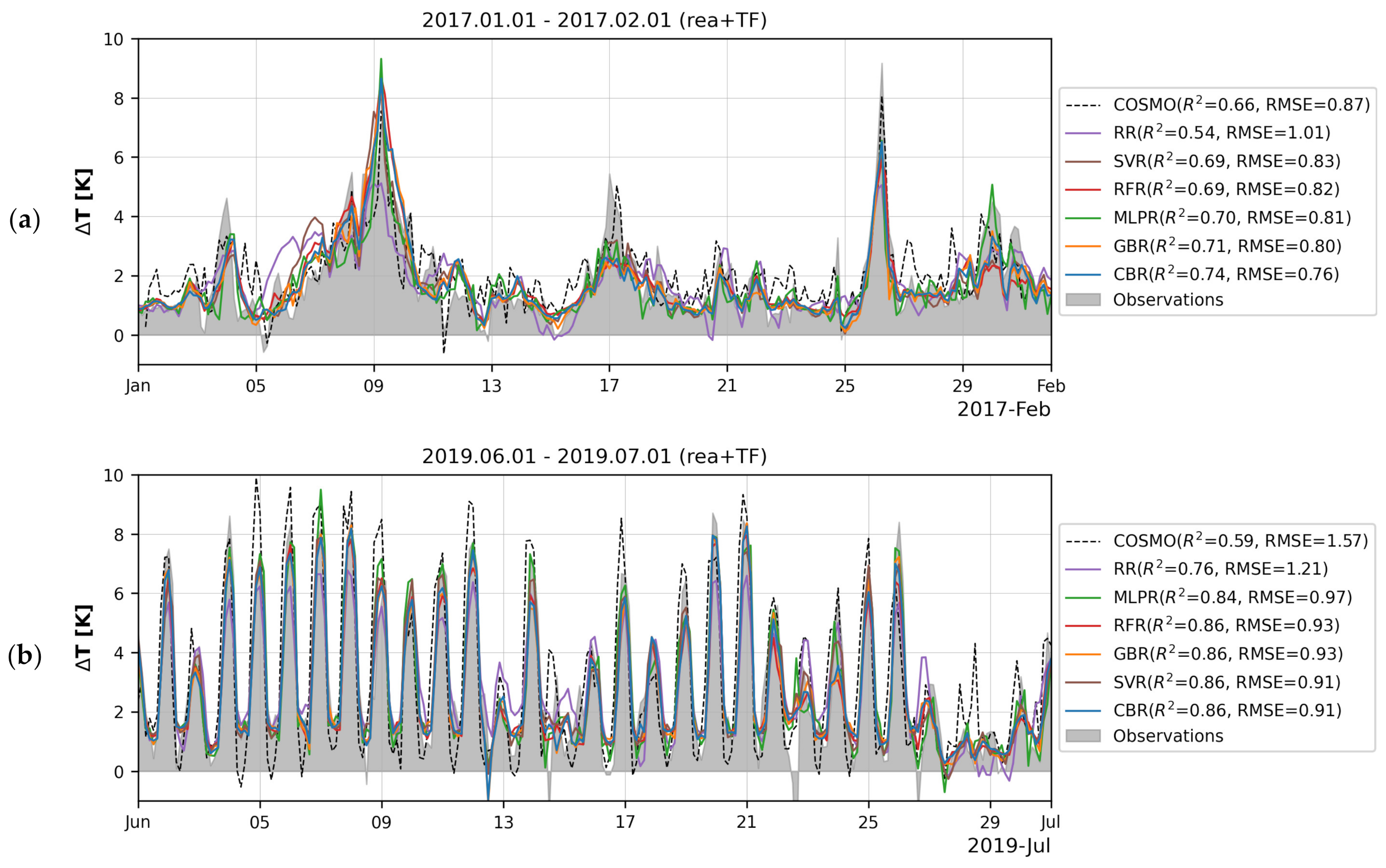
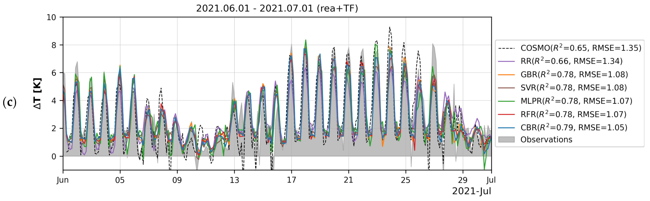
Table 1.
List of meteorological variables used as predictors for urban heat island (UHI) magnitude. Plus and minus signs indicate the presence of variables in observations and reanalysis.
Table 1.
List of meteorological variables used as predictors for urban heat island (UHI) magnitude. Plus and minus signs indicate the presence of variables in observations and reanalysis.
| Name | Description | Unit | Weather Station Observations | Reanalysis |
|---|---|---|---|---|
| t2m | Air temperature at 2-m height | °C | + | + |
| rh2m | Relative humidity at 2-m height | % | + | + |
| vel10m | Wind speed at 10-m height | m/s | + | + |
| Tcc | Total cloud cover fraction | unitless (0–1) | + | + |
| Lcc | Low cloud cover fraction | unitless (0–1) | + | + |
| Sp | Atmospheric pressure | hPa | − | + |
| Blh | Boundary layer height | m | − | + |
| Str | Net longwave radiation | W/m2 | − | + |
| ssr | Net shortwave radiation | W/m2 | − | + |
| strd | Downwelling longwave radiation | W/m2 | − | + |
| ssrd | Downwelling shortwave radiation | W/m2 | − | + |
| tp | 3-h precipitation sum | mm | − | + |
Table 2.
Sets of predictors used to approximate UHI magnitude. Plus and minus signs indicate the presence of the listed groups of predictors in the different sets.
Table 2.
Sets of predictors used to approximate UHI magnitude. Plus and minus signs indicate the presence of the listed groups of predictors in the different sets.
| ID | Set Name | Astronomical Predictors | Observations-Based Predictors | Reanalysis-Based Predictors | Temporal Features | Number of Features |
|---|---|---|---|---|---|---|
| 1a | obs | + | + | − | − | 9 |
| 1b | rea | + | − | + | − | 18 |
| 1c | obs&rea | + | + | + | − | 24 |
| 2a | obs + TF | + | + | − | + | 39 |
| 2b | rea + TF | + | − | + | + | 102 |
| 2c | obs&rea + TF | + | + | + | + | 138 |
Table 3.
List of ML models used in the study.
| Model Name | Acronym | Tuned Hyperparameters and Their Values | Used to Analyze Feature Importance |
|---|---|---|---|
| Ridge Regression (baseline) | RR | - | − |
| Random Forest Regression | RFR | n_estimators [100, 200, 500] | + |
| Gradient Boosting Regression | RBR | n_estimators [100, 200, 500, 1000] | + |
| CatBoost Regression | CBR | n_estimators [100, 200, 500, 1000, 2000] | + |
| Support Vector Regression | SVR | - | − |
| Multi-Layer Perceptron Regression | MLPR | hidden_layer_sizes [100 × 3, 100 × 5, 100 × 7, 200 × 3, 200 × 5, 200 × 7]; max_iter [200, 500, 1000] | − |
Disclaimer/Publisher’s Note: The statements, opinions and data contained in all publications are solely those of the individual author(s) and contributor(s) and not of MDPI and/or the editor(s). MDPI and/or the editor(s) disclaim responsibility for any injury to people or property resulting from any ideas, methods, instructions or products referred to in the content. |
© 2023 by the authors. Licensee MDPI, Basel, Switzerland. This article is an open access article distributed under the terms and conditions of the Creative Commons Attribution (CC BY) license (https://creativecommons.org/licenses/by/4.0/).
Share and Cite
MDPI and ACS Style
Varentsov, M.; Krinitskiy, M.; Stepanenko, V. Machine Learning for Simulation of Urban Heat Island Dynamics Based on Large-Scale Meteorological Conditions. Climate 2023, 11, 200. https://doi.org/10.3390/cli11100200
AMA Style
Varentsov M, Krinitskiy M, Stepanenko V. Machine Learning for Simulation of Urban Heat Island Dynamics Based on Large-Scale Meteorological Conditions. Climate. 2023; 11(10):200. https://doi.org/10.3390/cli11100200
Chicago/Turabian StyleVarentsov, Mikhail, Mikhail Krinitskiy, and Victor Stepanenko. 2023. "Machine Learning for Simulation of Urban Heat Island Dynamics Based on Large-Scale Meteorological Conditions" Climate 11, no. 10: 200. https://doi.org/10.3390/cli11100200
Note that from the first issue of 2016, this journal uses article numbers instead of page numbers. See further details here.