Climate Change and Extreme Events in Northeast Atlantic and Azores Islands Region

Abstract

In small island regions, the influence of climate change assumes particular relevance. In the Azores archipelago, made up of nine islands, the geographical circumstances, oceanic condition, territorial dispersion, land use model and other physiographic constraints reinforce and enhance the vulnerability of the islands to changes in current weather patterns. Coupled Model Intercomparison Phase 6 (CMIP6) projections are used for the northeast Atlantic region to evaluate daily extreme climate events in large scale for the Azores region. Results shows changes in the annual maximum number of consecutive dry days, the annual number of wet days, and especially in the annual number of tropical nights. Despite limitations due to the lack of spatial detail, the large-scale framework suggests changes that may be enhanced by topography, particularly with respect to precipitation. The conclusions point to the need to establish standard rules in the processes of design, reviewing and/or amending territorial management instruments at the municipal scale in the Autonomous Region of the Azores, with the goal of adapting to a different climate from the recent past.

1. Introduction

Global atmospheric temperature will continue to increase until the mid-21st century under all emissions scenarios considered. Thus, a global temperature increase of 1.5 °C and 2 °C is expected to be exceeded during the 21st century unless considerable reductions in carbon dioxide (CO₂) and other greenhouse gas emissions occur in the coming decades [1]. The Fifth Assessment Report (AR5) [2] of the Intergovernmental Panel on Climate Change (IPCC) has also highlighted that climate change is now affecting weather and climate extremes in all regions of the globe, such as increased heat waves, heavy rainfall and longer periods of drought. The IPCC Sixth Assessment Report (AR6) also confirmed that is virtually certain that the frequency and intensity of hot extremes increased, and those of cold extremes have decreased on the global scale since 1950.

However, global warming is not equally distributed around the globe [3]. The effects of global warming on the evolution and distribution of temperature and precipitation are not evident. A warmer atmosphere can hold more water vapor according to the Clausius–Clapeyron relationship (CC) [4]. However, while an increase in evaporation and therefore in the amount of water vapor in the atmosphere is expected, it is not clear whether this translates into an increase in precipitation [5]. Evaporation and precipitation processes are very complex, and the most advanced models still rely on parameterizations or coarse representations to resolve these mechanisms in the atmosphere [6,7].

Due to its particular geographical location, in the North Atlantic subtropical region, and in the path of many polar and tropical disturbances that eventually affect the European continent, the Azores islands have been, since the late 19th century, the object of scientific interest by the international meteorological community [8]. Its position close to the North Atlantic Subtropical Anticyclone, aka the Azores High, has made the Azores a reference in the characterization of the circulation patterns that control the weather in western Europe. The clearest example is the NAO (North Atlantic Oscillation) index created in 1923 by Gilbert Thomas Walker, which initially consisted of the difference in mean sea level pressure between Ponta Delgada (Miguel-Azores) and Reykjavik (Iceland) [9]. In this context and in the framework of climate change, several studies have already been carried out in the Azores using the results of Coupled Model Intercomparison Phase 5 (CMIP5) [8,10,11,12,13].

Coupled Ocean–Atmosphere Global Circulation Models (CGCMs) are based on the physical laws describing the dynamics of the atmosphere and the ocean expressed in the form of mathematical equations [14]. Since these equations are non-linear, they can only be solved numerically using classical mathematical methods and powerful computers [15]. Currently, CGCMs constitute a complete representation of the climate system, with an evolution towards more and more complex models that include biogeochemical cycles [16].

But the climate models need scenarios that condition their response. The SSP (Shared Socioeconomic Pathway) scenarios describe possible future climate scenarios, which depend on how socioeconomic factors may change in this century such as population, economic growth, education, urbanization and the rate of technological development [17]. Under these conditions, the SSP consist of five different ways in which the world may evolve in the absence of climate policies and how different levels of climate change mitigation can be achieved when the mitigation targets of the RCPs (Representative Concentration Pathways) are combined with the SSP [18].

The objective of Coupled Model Intercomparison (CMI) is to better understand past, present, and future climate change arising from natural, unforced variability or in response to changes in radiative forcings in a multi-model context [16]. CMI Phase 6 (CMIP6) brought an advanced understanding of the role of clouds in general atmospheric circulation and climate sensitivity to assess the response of the cryosphere to a warming climate and its global consequences; to understand the factors that control water availability over land; to assess climate extremes, what controls them, how they have changed in the past and how they might change in the future; to understand and predict regional sea level change and its coastal impacts; to improve near-term climate predictions; and to determine how biogeochemical cycles and feedback control greenhouse gas concentrations and climate change [16].

There are very few studies on projections of climate extremes in oceanic regions and even fewer on small islands. With regard to the improvements achieved by the CMIP6 models, the main motivation for this study is to evaluate the CMIP6 results for some extreme climate indices in the Azores region. To date, this is the first study on climate extremes in the Azores using CMIP6 results.

2. Materials and Methods

An area between 36.5° N–40° N and 32° W–24.5° W has been defined in the eastern North Atlantic, containing the Azores region (Figure 1). A larger area (30° N–50° N, 5° W–45° W) is also used to assess changes on a synoptic scale.

A set of 33 models of the CMIP6 project (

Table 1. CMIP6 models used in this work.

Model	Nominal Horizontal Resolution	Institution
ACCESS-CM2	250 km	CSIRO-ARCCSS
ACCESS-ESM1-5	250 km	CSIRO
AWI-ESM-1-1-LR	250 km	AWI
BCC-ESM1	250 km	BCC
CanESM5	500 km	CCCma
CESM2-FV2	250 km	NCAR
CESM2-WACCM	100 km	NCAR
CESM2	100 km	NCAR
CMCC-CM2-HR4	100 km	CMCC
CMCC-CM2-SR5	100 km	CMCC
CMCC-ESM2	100 km	CMCC
EC-Earth3-AerChem	100 km	EC-Earth-Consortium
EC-Earth3-CC	100 km	EC-Earth-Consortium
EC-Earth3-Veg-LR	250 km	EC-Earth-Consortium
FGOALS-f3-L	100 km	CAS
FGOALS-g3	250 km	CAS
GFDL-ESM4	100 km	NOAA-GFDL
IITM-ESM	250 km	CCCR-IITM
INM-CM4-8	100 km	INM
INM-CM5-0	100 km	INM
IPSL-CM5A2-INCA	500 km	IPSL
IPSL-CM6A-LR	250 km	IPSL
KACE-1-0-G	250 km	NIMS-KMA
KIOST-ESM	250 km	KIOST
MIROC6	250 km	MIROC
MPI-ESM1-2-HR	100 km	MPI-M
MPI-ESM1-2-LR	250 km	MPI-M
MRI-ESM2-0	100 km	MRI
NESM3	250 km	NUIST
NorCPM1	250 km	NCC
NorESM2-MM	100 km	NCC
SAM0-UNICON	100 km	SNU
TaiESM1	100 km	AS-RCEC

) was used in this work. However, not all the models have results for all the variables and/or all the scenarios simultaneously. Therefore, only subsets of these models were effectively used, depending on the variable and scenario used. Each model has a historical simulation, which consists of a reconstruction of the climatological series at each point of the globe, based on known boundary conditions over time (atmospheric composition, solar forcing, etc.), and several projections corresponding to the various SSP scenarios.

For all simulations, only the first variant ID “r1i1p1f1” was used because it is the most common one. The variant ID identifies the realization index (i.e., ensemble member), initialization method, physics version and forcing variant used in each simulation [19].

The historical simulations and projections datasets of CMIP6 used in this paper are available in the Climate Data Store (CDS) of the Copernicus program [20]. Global Climate Models have been used as a fundamental tool for the analysis of past and future climate extremes [21].

Table 2. CMIP6 models used in historical simulations. The “x” marks mean “available”.

Model	Daily Total Precipitation	Daily Minimum Temperature
ACCESS-CM2	x	x
ACCESS-ESM1-5	x	x
AWI-ESM-1-1-LR	x	x
BCC-ESM1	x	x
CanESM5	x	x
CESM2-FV2	x
CESM2-WACCM	x
CESM2	x
CMCC-CM2-HR4	x
CMCC-CM2-SR5	x
CMCC-ESM2	x	x
EC-Earth3-AerChem	x	x
EC-Earth3-CC	x	x
EC-Earth3-Veg-LR	x	x
FGOALS-f3-L	x	x
FGOALS-g3	x	x
GFDL-ESM4	x	x
IITM-ESM	x
INM-CM4-8	x	x
INM-CM5-0	x	x
IPSL-CM5A2-INCA	x
IPSL-CM6A-LR	x	x
KACE-1-0-G	x	x
KIOST-ESM	x	x
MIROC6	x	x
MPI-ESM1-2-HR	x	x
MPI-ESM1-2-LR	x	x
MRI-ESM2-0	x	x
NESM3	x	x
NorCPM1	x	x
NorESM2-MM	x	x
SAM0-UNICON	x	x
TaiESM1	x

shows the CMPI6 models used for historical simulations of daily precipitation amounts and daily minimum temperature. All the models present results for total daily precipitation, while only 25 present results for minimum daily temperature. On the other hand, not all models have the same spatial resolution. To enable comparisons with the reference, the ERA5 reanalysis [22], it was necessary to regrid the fields to the same spatial resolution as ERA5 (0.25° × 0.25°).

In this work we used three SSP scenarios: SSP1 2.6, SSP2 4.5 and SSP5 8.5. These represent low, intermediate and high radiative forcings due to different greenhouse gases emission pathways. As not all the models have results for all the available SSP scenarios, those that maximized the number of models available for the chosen variables were selected.

Table 3. CMIP6 models used in SSP scenarios projections. The “x” marks mean “available”.

Model	SSP1 2.6	SSP2 4.5	SSP5 8.5
ACCESS-CM2	x	x	x
AWI-CM-1-1-MR	x	x	x
BCC-CSM2-MR	x	x	x
CanESM5	x	x	x
CESM2-WACCM			x
CMCC-CM2-SR5		x	x
CMCC-ESM2	x	x	x
EC-Earth3-CC		x	x
EC-Earth3-Veg-LR	x	x	x
FGOALS-g3	x	x	x
GFDL-ESM4	x	x	x
IITM-ESM	x	x	x
INM-CM4-8	x	x	x
INM-CM5-0	x	x	x
IPSL-CM5A2-INCA	x
IPSL-CM6A-LR	x	x	x
KACE-1-0-G	x	x	x
KIOST-ESM	x	x	x
MIROC6	x	x	x
MPI-ESM1-2-LR	x	x	x
MRI-ESM2-0	x	x	x
NESM3		x	x
NorESM2-LM	x	x	x
NorESM2-MM	x	x	x
TaiESM1			x

shows the models used for each SSP scenario. As can be seen, 25 models were used, but not all scenarios are available.

Daily data downloaded from “CMIP6 climate projections” CDS [23] consist of historical and projection simulations for two climate elements: daily total precipitation (PRECTOT) and minimum daily temperature (TNM). Three extreme climate indices, CDD (annual number of consecutive dry days), R20 mm (annual number of wet days) and TR (annual number of tropical nights), as well as ensemble means and ranges were computed using the python climate tools in the XCLIM module [24]. As a reference dataset, “ERA5 hourly data on single levels” hourly data from 1961 to 1990 were downloaded from CDS. Daily total precipitation and daily minimum temperatures were computed, as well as the three extreme climate indices mentioned above.

Spatial averages of ERA5 and CMIP6 were performed in the working area defined as “Azores region”, i.e., between 36.5° N–40° N and 32° W–24.5° W (Figure 1), to compute time series, bias, trends and changes. Biases between the CMPI6 ensemble mean of historical and ERA5 reference datasets were evaluated in the region under study, as well as the linear trends and changes projected for the end of the century, 2071–2100, with respect to the 1961–1990 ERA5 reference period.

All calculated p-values refer to t-tests. For biases, the null hypothesis is that 2 independent samples have identical (expected) mean values and assume identical variances. For trends, the null hypothesis is that the slope is zero, using the Wald test with the t distribution of the test statistic. The results are considered statistically significant when the p-values are less than 0.05, i.e., when the confidence interval is 95%.

3. Results

3.1. Atmospheric CO₂

Data of monthly averages of CO₂ mole fraction measured in air samples collected at Serreta station (Terceira Is. Azores, AZR: 38.770000° N, 27.379999° W) from 1980 to 2022 were downloaded from the WMO World Data Centre for Greenhouse Gases (WDCGG) [25]. The samples were collected by the IPMA (Portuguese Institute for Sea and Atmosphere) and analyzed by Global Monitoring Laboratory (NOAA). Longitude-averaged data of historical and projections simulations were also downloaded from the CMIP6 Forcing Datasets (input4MIPs) at the World Data Center for Climate, including historical data [26] (1850–2014) and projections (2015–2100) for the three scenarios: SSP1 2.2 [27], SSP2 4.5 [28] and SSP5 8.5 [29]. The data obtained have a resolution of 0.5°, and linear interpolation was applied to obtain the time series at the Serreta latitude (38.77° N).

Figure 2 presents the time series of monthly averages of measurements of the mole fraction of atmospheric CO₂ from air samples collected at Serreta station (38.77° N) from 1980 to 2022 and estimated for the same latitude, according to historical simulations (until 2014) and projections until 2100 and for the three scenarios, SSP1 2.2, SSP2 4.5 and SSP5 8.

The three scenarios follow almost identical trajectories until about 2024, diverging afterwards almost exponentially. While in the SPP2 4.5 scenario, CO₂ abundance tends to a value of about 600 ppm(v), and in the SSP1 2.6 scenario, a maximum is reached by 2060. On the other hand, the SSP5 8.5 scenario’s trajectory increases exponentially. CO₂ historical simulation shows a non-statistically significant (p-value < 0.05) positive bias of 1.39 ± 2.48 ppm relative to ERA5, whereas both show significant trends for the period of 1980–2024 (

Table 4. Linear trends of CO₂ at Serreta (1980–2014).

	Trend (ppm/Year)
Measurements	1.73 ± 0.03
Historical	1.85 ± 0.03

).

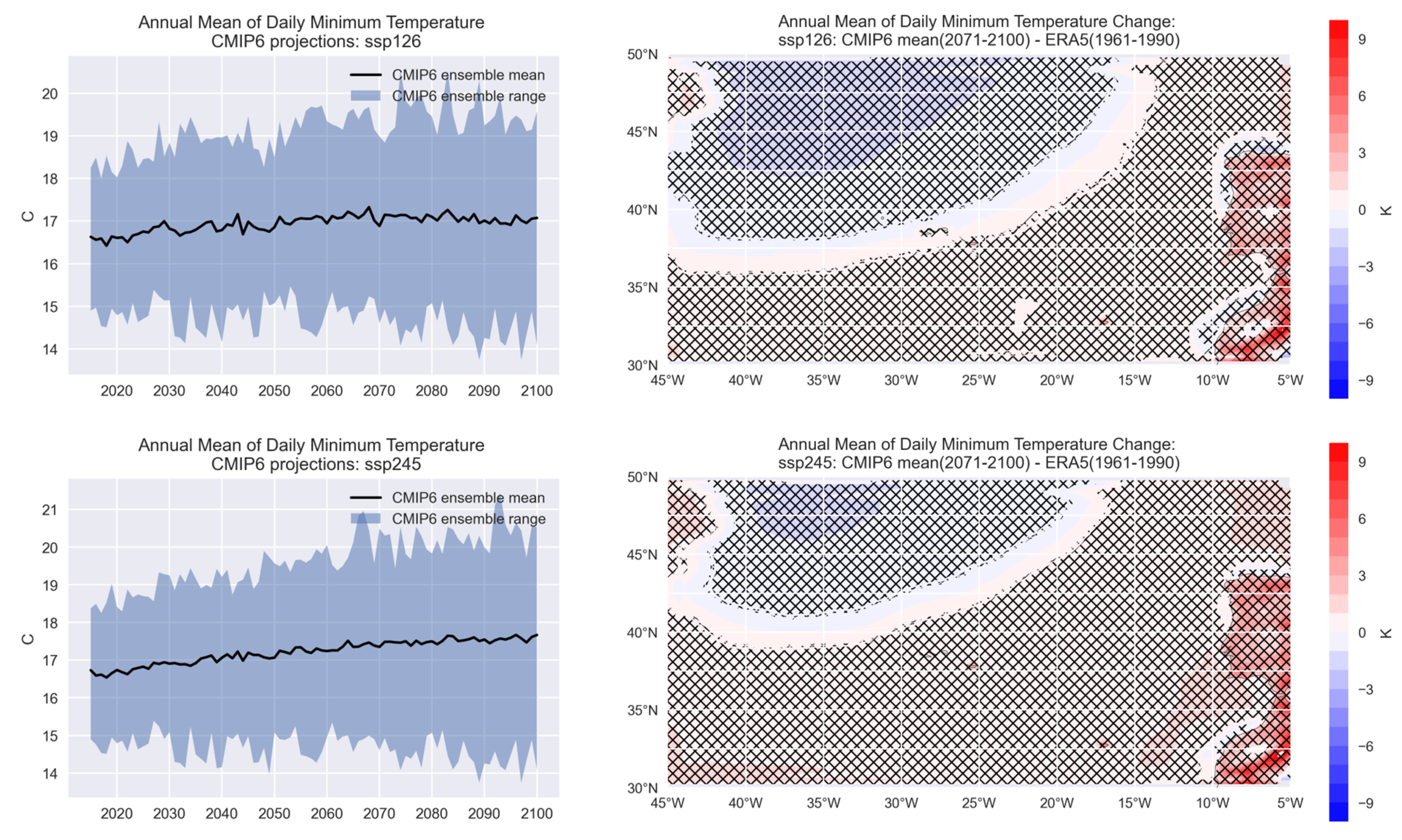
3.2. Annual Mean of Daily Minimum Temperature

Historical annual means of daily minimum temperature simulated by CMIP6 models were compared with ERA5 reanalysis data. Figure 3 shows the departure of CMIP6 simulations from ERA5 during the 1961–1990 reference period. The results show a small but statistically significant (p-value < 0.05) bias of −0.56 ± 0.27 K in the region. This means that CMIP6 simulations systematically underestimate ERA5 reference data, with ERA5 data being inside the amplitude range of the CMPI6 ensemble. This is true not only in the Azores region but also for most part of the Northeastern Atlantic and adjacent continental regions (Figure 4). The CMIP6 ensemble mean shows a statistically significant (p-value < 0.05) positive linear trend of 0.038 ± 0.003 K/decade from 1850 to 2014. However, as can be seen, the majority of the increase occurred during the last 30 years.

CMIP6 projections of the annual mean of the daily minimum temperature for the three SSP scenarios were also compared to the 1961–1990 ERA5 reference period. The left column of Figure 5 shows the ensemble means and ranges of the annual mean of the daily minimum temperature for each of the three scenarios. These results show positive trends of mean and amplitude ranges of the ensembles in all scenarios, especially in SSP2 4.5 and SSP5 8.5 (

Table 5. CMPI6 ensemble mean projections of annual mean daily minimum temperature for the Azores region. Linear trends (2015–2100) and projected changes (Δ) for 2071–2100 relative to 1961–1990.

Scenario	Trend (K/Decade)	Trend p-Value	Δ (K)	Δ p-Value
ssp126	0.055 ± 0.006	3.68 × 10−15	0.073 ± 0.289	1.72 × 10−1
ssp245	0.118 ± 0.004	5.14 × 10−47	0.539 ± 0.293	1.08 × 10−14
ssp585	0.225 ± 0.003	1.91 × 10−79	1.221 ± 0.347	2.01 × 10−27

).

The right column of Figure 5 shows maps of the CMIP6-projected change in the annual mean daily minimum temperature for the end of XXI century (2071–2100) relative to the 1961–1990 ERA5 reanalysis and for each scenario. CMIP6 projections were bias-adjusted using the results of the 1961–1990 comparison, and statistically significant (p-value < 0.05) areas are represented with hatches. It can be seen that the projected changes are positive for all the scenarios and for most of the north-east Atlantic, but the SSP1 2.6 scenario is not statistically significant in the Azores region, except for the islands. These results are summarized in Table 5.

Comparatively, higher values are observed in the Iberian Peninsula and North Africa; it can also be seen in both continental regions that this increase is boosted by distance from the sea.

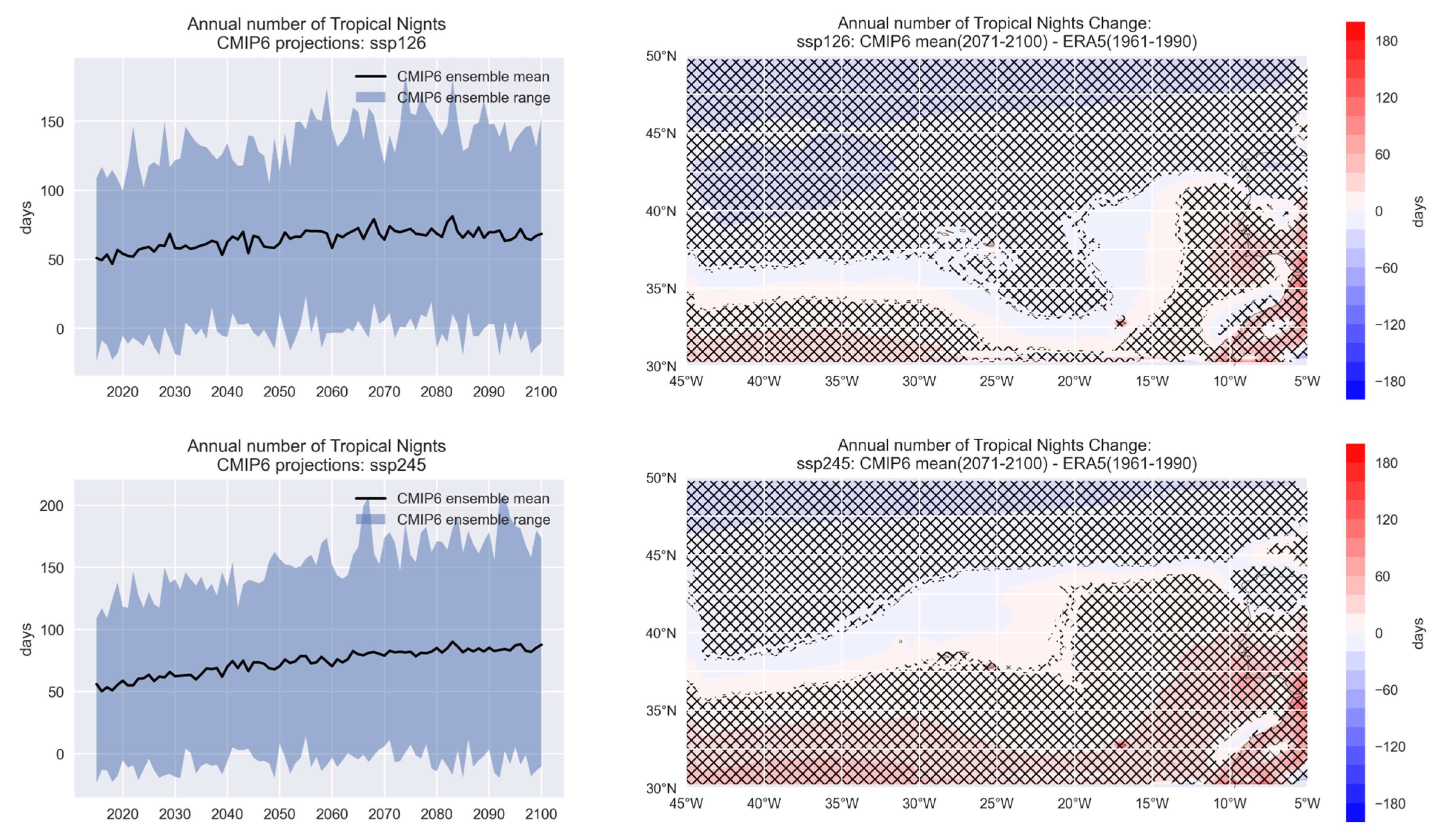
3.3. Annual Number of Tropical Nights

Similarly, CMIP6 projections of the annual number of tropical nights for the three SSP scenarios were also compared to the 1961–1990 ERA5 reference period. The annual number of tropical nights ($TR$) is defined as the annual count of days when $TN$ (daily minimum temperature) > 20 °C. Let ${TN}_{ij}$ be the daily minimum temperature on day i in year j. $TR$ is the count of days where:

$${ TN}_{ij}>20 °\mathrm{C}$$

Comparisons between CMIP6 simulations of historical data and ERA5 reanalysis between 1961 and 1990 show a statistically significant bias of −26.0 ± 12.2 tropical nights, i.e., the simulations underestimate the reanalysis in the Azores region. Figure 6 shows the TR time series computed from ERA5 daily minimum temperatures and CMIP6 hourly temperatures from 1961 to 1990, where almost all ERA5 data are above the CMIP6 mean values but still inside the range.

The left column of Figure 7 shows the ensemble means and ranges of $TR$ for the three SSP scenarios. As expected, these results show positive and statistically significant trends of mean and amplitude ranges of the ensembles in all scenarios (

Table 6. CMPI6 ensemble mean projections of annual number of tropical nights for the Azores region. Linear trends (2015–2100) and projected changes (Δ) for 2071–2100 relative to 1961–1990.

Scenario	Trend (Day/Decade)	Trend p-Value	Δ (Day)	Δ p-Value
ssp126	0.20 ± 0.02	1.21 × 10−14	−7.57 ± 12.57	1.38 × 10−3
ssp245	0.38 ± 0.01	2.47 × 10−41	6.71 ± 12.03	3.23 × 10−3
ssp585	0.72 ± 0.01	5.48 × 10−74	28.15 ± 12.56	8.69 × 10−17

). However, SSP1 2.6 shows a negative change that is consistent with an expected decrease in TR at the end of the century. The right column of Figure 7 shows maps of the CMIP6-projected change in TR for the end of XXI century relative to the 1961–1990 ERA5 reanalysis and for each scenario. In the CMIP6 projections, statistically significant (p-value < 0.05) areas are represented with hatches. It can be seen that the projected changes are positive for all the scenarios and for most of the north-east Atlantic, but the SSP1 2.6 and SSP2 4.5 scenarios are partially statistically significant in the Azores region.

3.4. Annual Total Precipitation Amount

The annual total precipitation amount computed from daily PRECTOT CMIP6 historical simulations data were compared to ERA5 reanalysis data computed from hourly datasets. Figure 8 shows the departures of CMIP6 simulations from ERA5 during the 1961–1990 reference period. The results show a small but non-statistically significant (p-value = 0.78) bias of −6.3 ± 123.7 mm in the region. This means that CMIP6 ensemble mean is very close to ERA5 reference data, i.e., there is no statistically significant difference between the two sets. However, there are large areas with either a large positive or negative bias in the Northeastern Atlantic and in continental regions (Figure 9). The CMIP6 ensemble mean (Figure 8) shows a small but statistically significant (p-value < 0.05) positive linear trend of 0.038 ± 0.003 mm/decade from 1850 to 2014.

In addition, the annual precipitation amount in CMIP6 simulations of historical data and ERA5 data between 1961 and 1990 show a small bias of −6.3 ± 123.8 mm, which is not statistically significant in the Azores region.

Figure 10 (left column) shows the ensemble means and ranges of the annual mean of the daily minimum temperature for each of the three scenarios. These results show small positive but statistically significant trends in the mean and amplitude ranges of the ensembles in all scenarios, and for SSP1 2.6 and SSP2 4.5 (

Table 7. CMPI6 ensemble mean projections of annual total precipitation amount for the Azores region. Linear trends (2015–2100) and projected changes (Δ) for 2071–2100 relative to 1961–1990.

Scenario	Trend (mm/Decade)	Trend p-Value	Δ (K)	Δ p-Value
ssp126	3.79 ± 1.33	5.65 × 10−3	18.5 ± 126.9	4.31 × 10−1
ssp245	2.11 ± 0.89	2.01 × 10−2	7.2 ± 126.4	7.55 × 10−1
ssp585	−1.23 ± 0.69	7.84 × 10−2	−10.1 ± 126.0	6.60 × 10−1

). However, SSP5 8.5 shows a negative and statistically significant trend. The right column of Figure 10 shows maps of the CMIP6–projected change of annual total precipitation amount for the end of XXI century (2071–2100) relative to the 1961–1990 ERA5 reanalysis and for each scenario. CMIP6 projections were bias-adjusted using the results of the 1961–1990 comparison, and statistically significant (p-value < 0.05) areas are represented with hatches. It can be noted that the maps of projected change maps are very similar, and that changes are small and not statistically significant (p-value > 0.05) for the Azores region and for all the scenarios. However, there are large areas where changes are large and either positive or negative in the north-east Atlantic.

3.5. Annual Number of Consecutive Dry Days

CMIP6 projections of the annual number of consecutive dry days for the three SSP scenarios were also compared to the 1961–1990 ERA5 reference period. The annual number of consecutive dry days ($CDD$) is defined as the annual maximum number of consecutive days with $\mathrm{P}\mathrm{R}\mathrm{E}\mathrm{C}\mathrm{T}\mathrm{O}\mathrm{T}<1 \mathrm{m}\mathrm{m}$. Let ${ RR}_{ij}$ be the daily precipitation amount on day i in year j. CDD is the largest number of consecutive days, where

$${ RR}_{ij}<1 \mathrm{m}\mathrm{m}$$

Simulations of historical data of the annual number of consecutive dry days from CMIP6 ensembles and ERA5 data between 1961 and 1990 (Figure 11) show a small non-statistically significant bias of 0.61 ± 5.3 days in the Azores region. The left column of Figure 12 shows the ensemble means and ranges of CDD for the three SSP scenarios. These time series show small negative trends in the ensembles means in the SSP1 2.6 and SSP2 4.5 scenarios (Table 7) in the 2015–2100 period. However, the SSP2 4.5 trend is not statistically significant (p-value > 0.05), but that of SSP5 8.5 shows a statistically significant positive trend.

The right column of Figure 12 shows maps of the CMIP6-projected changes of $CDD$ for the end of XXI century relative to 1961–1990 ERA5 and for each scenario. Statistically significant (p-value < 0.05) areas are represented with hatches. The projected changes are positive and statistically significant for all the scenarios for the Azores region (

Table 8. CMPI6 ensemble mean projections of annual number of consecutive dry days for the Azores region. Linear trends (2015–2100) and projected changes (Δ) for 2071–2100 relative to 1961–1990.

Scenario	Trend (Day/Decade)	Trend p-Value	Δ (Day)	Δ p-Value
ssp126	−0.19 ± 0.06	1.24 × 10−3	2.83 ± 5.20	4.83 × 10−3
ssp245	−0.02 ± 0.04	5.97 × 10−1	3.78 ± 5.01	2.06 × 10−4
ssp585	0.27 ± 0.03	1.19 × 10−13	5.64 ± 4.96	1.62 × 10−7

). However, a closer view of the maps show that the Western group (Flores and Corvo islands) and Eastern Group (São Miguel and Santa Maria islands) are on the border of the statistically significant positive trends, but the Central Group (Terceira, Graciosa, Faial, Pico and São Jorge islands) is always in the non-significant zone.

3.6. Annual Number of Wet Days

CMIP6 projections of annual number of wet days for the three SSP scenarios were also compared with 1961–1990 ERA5 reference period. The annual number of wet days ($R20 \mathrm{m}\mathrm{m}$) is defined as the annual count of days when PRECTOT ≥ 20 mm: Let ${ RR}_{ij}$ be the daily precipitation amount on day i in year j. $R20 \mathrm{m}\mathrm{m}$ is the number of days where:

$${ RR}_{ij} \ge 20 \mathrm{m}\mathrm{m}$$

Annual number of wet days from historical data simulations of CMIP6 ensembles and ERA5 data between 1961 and 1990 (Figure 13) show a non-statistically significant small bias of −0.16 ± 1.80 days in the Azores region.

Left column of Figure 14 show the ensemble means and ranges of $R20 \mathrm{m}\mathrm{m}$ for the three SSP scenarios. The time series show small trends but statistically significant in all scenarios (

Table 9. CMPI6 ensemble mean projections of annual number of wet days for the Azores region. Linear trends (2015–2100) and projected changes (Δ) for 2071–2100 relative to 1961–1990.

Scenario	Trend (Day/Decade)	Trend p-Value	Δ (Day)	Δ p-Value
ssp126	0.077 ± 0.021	5.25 × 10−4	1.0 ± 1.8	4.44 × 10−3
ssp245	0.082 ± 0.015	4.09 × 10−7	1.1 ± 1.9	2.26 × 10−3
ssp585	0.080 ± 0.012	9.97 × 10−10	1.1 ± 1.9	1.35 × 10−3

). Right column of Figure 14 show maps of the CMIP6-projected change of $R20 \mathrm{m}\mathrm{m}$ for the end of XXI century relative to 1961–1990 ERA5 and for each scenario, where areas where statistically significant (p-value < 0.05) are represented with hatches. Northern areas have positive significant changes, while southern areas have negative significant changes. A closer look at the Azores region shows significant positive changes in the Western and Central Groups and non-significant positive changes in the Eastern Group for the three scenarios.

4. Discussion

The results of the historical CO₂ mole fraction simulations for the Azores coincide with those observed at the Serreta station and indicate a statistically significant increasing trend between 1980 and 2022. The projections between 2022 and 2100 based on the three scenarios used suggest that the differentiation between the scenarios should occur from 2024 onwards (Figure 2). This result demonstrates that background CO₂ has a homogeneous global distribution that varies with latitude and the importance of monitoring in atmospheric background conditions. However, if the simulated atmospheric CO₂ coincides with the values observed in the Azores, this does not mean that the same is true of the air temperature or the amount of precipitation.

Results show that the CMIP6 ensemble mean of historical simulations of the annual mean of the daily minimum temperature show statistically significant biases for the Azores region and for other regions of the Northeast Atlantic (Figure 3). For the Azores region, the ensemble mean of the simulations of the annual averages of minimum daily temperature (TNM) from CMIP6 systematically underestimate the reference (ERA5), while for the annual amount of precipitation (PRECPTOT), the bias is not significant. A small underestimation of the TNM has a significant impact on the annual number of tropical nights (TR). A relatively small bias of 0.56 K in annual mean of TNM leads to 26 days of TR. The CMIP6 bias spatial distribution of TNM is relatively homogeneous and negative over the Northeastern Atlantic, while it is generally positive and irregular over the continental areas (Figure 4).

For PRECPTOT, the bias field is less homogeneous over the ocean. It is negative near the North American coast, Morocco and the adjacent ocean, and some parts of coastal zones of the Iberian Peninsula, while positive in some inner parts of Iberian Peninsula and the adjacent northern ocean. Between these two areas of different bias signals, a small bias boundary crosses the ocean, including the Central Group of the Azores islands. This suggests that the CMIP6 models perform well for precipitation in the subtropical North Atlantic, along the northern branch of the Azores High.

Spatial averages over the Azores region of TNM and TR projections show positive and statistically significant trends for the period of 2015–2100 and for all the scenarios (Table 5 and Table 6). However, TR projections for the 1961–1990 to 2071–2100 periods show very different variations in the Azores region, depending on the adopted scenario, from a negative change of −8 days in SSP1 2.6 to 28 days in SSP5 8.5. TR shows an almost zonal distribution pattern, with positive changes in the southern and continental zones and negative changes in the northern and oceanic zones (Figure 7). The area of positive changes increases as the forcing increases. The increase in the TR ensemble mean in the Azores region is followed by an increase in the range amplitude, suggesting that there are solutions that can vary from zero to almost 300 days by the end of the century.

Computed CDD and R20 mm from CMIP6 simulations of historical data of PRCPTOT over the Azores (Figure 11 and Figure 13) show small and statistically non-significant bias from ERA5 reanalysis data. Positive and statistically significant trends (2015–2100) of PRCPTOT are found in the Azores region for scenarios SSP1 2.6 and SSP2 4.5 (Table 7). SSP5 8.5 shows a negative but non-significant trend, suggesting a growing uncertainty as the forcing scenario increases. The CDDs calculated from CMIP6 PRCPTOT projections show negative trends for SSP1 2.6 and SSP2 4.5 and positive trends for SSP5 8.5. The trend for SSP2 4.5 is not statistically significant and therefore the trend seems to increase and become more significant with the forcing scenario (Table 8). Projected changes for the end of the XXI century show positive and statistically significant small values in the Azores region. However, the islands of the Central Group are within a zone of non-significant change in all scenarios (Figure 12).

The R20 mm projections show more consistent results than CDD. Positive linear trends for all scenarios in the Azores region are small but statistically significant (Table 9). The same is true of the changes projected for the end of the 21st century. However, the spatial distribution of the changes shows that these changes are mostly in the areas of the Western and Central groups (Figure 13).

Comparisons with earlier results from CMIP5 [13], using RCP scenarios and different reference periods, suggest that CMIP6-projected temperature changes are positive but lower than those projected by CMIP5. Consequently, TR-projected changes from CMIP6 are lower those from CMIP5. On the other hand, the results of the CMIP6 projections of changes in annual precipitation amount are more negative than those of CMIP5. Consequently, the CDD and R20 mm projections are positive and higher in the CMIP6 than in the CMIP5.

Unfortunately, we have not found any evaluations in the literature of CMIP6 or CMIP5 projections of extremes in oceanic regions, and even less so on small islands, so we cannot compare the results obtained here. However, in general terms, the projections of air temperature and precipitation for the Northeast Atlantic region are consistent with the results obtained here [1].

The CMIP6 projections reflect changes in large-scale features, so these results only show the trends of these changes in the Azores region as a whole and not for each island individually, and there may be significant differences in both magnitude and direction depending mainly on the physiographic characteristics of each island. On the other hand, the CMIP6 results are the average of a set of individual model projections, and therefore, the amplitudes of changes from year to year are naturally smoothed. Therefore, while trends are useful for assessing local changes, some caution should be exercised with individual years when applying to a specific site or location. In addition, the methodology adopted only allows us to make inferences about annual trends and changes, and therefore, it is not possible to assess trends or seasonal changes with these results.

ERA5’s resolution for the Azores region is approximately 28 km in latitude × 22 km in longitude. Only the islands of São Miguel, Pico, Terceira and São Jorge are larger than this resolution, although ERA5 does show some relief on the islands of the westernmost group (Flores and Corvo). In general, ERA 5’s topographic representation underestimates the real topography of the islands. For example, the highest elevation in ERA5 in the Azores region is 116 m on the island of São Miguel, while the highest altitude on the island of São Miguel is 1103 m. On the other hand, the highest elevation in the Azores is located on the island of Pico (2351 m), but the ERA shows a maximum of 80 m for the same point. As for the CMIP6 models, the nominal resolution is even lower (100 km to 500 km), while the largest island in the Azores (São Miguel) is only 64 km long. Most of the models show maximum altitudes of between 3 and 27 m, centered on the Central Group, but there are some that do not show any elevation in the region (ACCESS-CM2, ACCESS-ESM1-5, CMCC-CM2-SR5, CMCC-ESM2, INM-CM4-8 and INM-CM5-0). On the other hand, all of the elevations of the CMIP6 models underestimates ERA5 by at least 100 m.

On islands with higher mountains (ex., S, Miguel, Terceira and Pico) orographic forcing is an important mechanism for precipitation occurrence and therefore leads to an increase in heavy rainfall episodes [30,31]. In the case of flatter islands (ex. S. Maria and Graciosa) can have longer drought periods. Thus, topographic differences can lead to enhanced differences in precipitation extremes between islands, leading to disruptive effects in vulnerable systems like Azores.

Positive trends on the length of the drought periods can impact native and endemic species, while positive trends on heavy rain events can impact the safety of populations. Positive trends of tropical nights can impact cause-specific mortality [32,33].

Extreme weather events increase due to climate change are no exception for Azores, and impacts on human and planetary health are also expected [34]. The survival areas of some native and endemic species may also be threatened by climate change.

Other important sectors for the economy of the Azores, such as agriculture, livestock, fisheries and tourism, may suffer significant impacts as a result of the increased risk of natural disasters arising from these changes, especially in isolated and small regions, where recovery is usually more costly and time-consuming [30,31].

5. Conclusions

The results obtained allow us to conclude the following:

• The increase in CO₂ observed in the Azores coincides with that estimated for the same latitude. The current SSP pathway can be identified from 2024 onwards.
• The annual average daily minimum temperature projected by the CMIP6 models in the Azores presents a significant bias compared to the ERA5 reference. This is also true to most part of the Northeast Atlantic area.
• The estimated annual precipitation total for the Azores does not show a significant bias compared to the ERA5 reference. However, there are zones of significant positive and negative bias in Northeast Atlantic area.
• Projections of annual average daily minimum temperatures in the Azores region suggest that an increase in annual average daily temperatures during this century is likely for the SSP1 2.6 scenario and very likely for the remainder. An increase in the annual number of tropical nights is also very likely in all scenarios.
• The annual precipitation projections show no significant changes. The increases in CDD and R20 mm are small but very likely for the SSP 5 8.5 scenario. These results suggest that a simultaneous increase in these two indices and in air temperature means that the CC relationship should be the dominant process in a worst-case forcing scenario, especially in the western islands.

References

1. Intergovernmental Panel on Climate Change. Climate Change 2021—The Physical Science Basis; Cambridge University Press: Cambridge, UK, 2023; ISBN 9781009157896. [Google Scholar]
2. Intergovernmental Panel on Climate Change. Climate Change 2013—The Physical Science Basis; Cambridge University Press: Cambridge, UK, 2014; ISBN 9781107057999. [Google Scholar]
3. Summary for Policymakers. In Global Warming of 1.5 °C; Cambridge University Press: Cambridge, UK, 2022; pp. 1–24.
4. Wallace, J.M.; Hobbs, P.V. Atmospheric Science: An Introductory Survey: Second Edition; Elsevier Inc.: Amsterdam, The Netherlands, 2006; ISBN 9780127329512. [Google Scholar]
5. Schneider, T.; O’Gorman, P.A.; Levine, X.J. Water Vapor and the Dynamics of Climate Changes. Rev. Geophys. 2010, 48, 1–22. [Google Scholar] [CrossRef]
6. Stensrud, D.J. Parameterization Schemes: Keys to Understanding Numerical Weather Prediction Models; Cambridge University Press: Cambridge, UK, 2009; ISBN 9780521865401. [Google Scholar]
7. Feingold, G. Parameterization of the Evaporation of Rainfall for Use in General Circulation Models. J. Atmos. Sci. 1993, 50, 3454–3467. [Google Scholar] [CrossRef]
8. Meirelles, M.G.; Carvalho, F.R. Perspectives of atmospheric sciences in the Azores: History of meteorology and climate change. In Archipelagos. Types, Characteristics and Conservation; Perez, M., Mills, J., Eds.; NOVA, Science Publishers: New York, NY, USA, 2019; pp. 43–69. ISBN 978-1-53614-682-0. [Google Scholar]
9. Stephenson, D.B.; Wanner, H.; Brönnimann, S.; Luterbacher, J. The History of scientific research on the North Atlantic oscillation. In Geophysical Monograph Series; Blackwell Publishing Ltd.: Hoboken, NJ, USA, 2003; Volume 134, pp. 37–50. ISBN 9781118669037. [Google Scholar]
10. Meirelles, M.; Carvalho, F.; Porteiro, J.; Henriques, D.; Navarro, P.; Vasconcelos, H. Climate Change and Impact on Renewable Energies in the Azores Strategic Visions for Sustainability. Sustainability 2022, 14, 15174. [Google Scholar] [CrossRef]
11. Carvalho, F.; Meirelles, M.; Henriques, D.; Navarro, P. Alterações Climáticas e o Aumento de Eventos Extremos Nos Açores. Bol. Núcleo Cult. Horta 2020, 29, 95–108. [Google Scholar]
12. Carvalho, F.; Meirelles, M.; Henriques, D.; Navarro, P. Alterações Climáticas e Energia No Contexto Dos Açores. Bol. Núcleo Cult. Horta 2020, 29, 95–108. [Google Scholar]
13. Carvalho, F.R.S.; Meirelles, M.G.; Henriques, D.V.; Navarro, P.V.; Vasconcelos, H.C. Climate change and the increase of extreme events in Azores. In Climate Change Management; Springer Science and Business Media: Berlin/Heidelberg, Germany, 2022; pp. 349–365. [Google Scholar]
14. Peixoto, J.P.; Oort, A.H. Physics of Climate; Springer: Berlin/Heidelberg, Germany, 1992; ISBN 978-0-88318-712-8. [Google Scholar]
15. Mcavaney, B.J.; Holland, G.J. Dynamics of future climates. In World Survey of Climatology; Elsevier: New York, NY, USA, 1995; pp. 281–314. [Google Scholar]
16. Eyring, V.; Bony, S.; Meehl, G.A.; Senior, C.A.; Stevens, B.; Stouffer, R.J.; Taylor, K.E. Overview of the Coupled Model Intercomparison Project Phase 6 (CMIP6) Experimental Design and Organization. Geosci. Model Dev. 2016, 9, 1937–1958. [Google Scholar] [CrossRef]
17. O’Neill, B.C.; Kriegler, E.; Riahi, K.; Ebi, K.L.; Hallegatte, S.; Carter, T.R.; Mathur, R.; van Vuuren, D.P. A New Scenario Framework for Climate Change Research: The Concept of Shared Socioeconomic Pathways. Clim. Change 2014, 122, 387–400. [Google Scholar] [CrossRef]
18. O’Neill, B.C.; Tebaldi, C.; van Vuuren, D.P.; Eyring, V.; Friedlingstein, P.; Hurtt, G.; Knutti, R.; Kriegler, E.; Lamarque, J.-F.; Lowe, J.; et al. The Scenario Model Intercomparison Project (ScenarioMIP) for CMIP6. Geosci. Model Dev. 2016, 9, 3461–3482. [Google Scholar] [CrossRef]
19. Taylor, K.E.; Juckes, M.; Balaji, V.; Cinquini, L.; Durack, P.J.; Elkington, M.; Guilyardi, E.; Kharin, S.; Lautenschlager, M.; Lawrence, B.; et al. CMIP6 Global Attributes, DRS, Filenames, Directory Structure, and CV’s. Available online: http://goo.gl/v1drZl (accessed on 4 November 2023).
20. Sandstad, M.; Schwingshackl, C.; Iles, C. Climate Extreme Indices and Heat Stress Indicators Derived from CMIP6 Global Climate Projections. Copernicus Climate Change Service (C3S) Climate Data Store (CDS). Available online: https://cds.climate.copernicus.eu/cdsapp#!/dataset/10.24381/cds.776e08bd?tab=overview (accessed on 1 June 2022).
21. Kim, Y.-H.; Min, S.-K.; Zhang, X.; Sillmann, J.; Sandstad, M. Evaluation of the CMIP6 Multi-Model Ensemble for Climate Extreme Indices. Weather Clim. Extrem. 2020, 29, 100269. [Google Scholar] [CrossRef]
22. Hersbach, H.; Bell, B.; Berrisford, P.; Hirahara, S.; Horányi, A.; Muñoz-Sabater, J.; Nicolas, J.; Peubey, C.; Radu, R.; Schepers, D.; et al. The ERA5 Global Reanalysis. Q. J. R. Meteorol. Soc. 2020, 146, 1999–2049. [Google Scholar] [CrossRef]
23. Copernicus Climate Change Service CMIP6 Climate Projections. Climate Data Store 2021. Available online: https://cds.climate.copernicus.eu/cdsapp#!/dataset/projections-cmip6?tab=overview (accessed on 6 October 2023).
24. Bourgault, P.; Huard, D.; Smith, T.J.; Logan, T.; Aoun, A.; Lavoie, J.; Dupuis, É.; Rondeau-Genesse, G.; Alegre, R.; Barnes, C.; et al. Xclim: Xarray-Based Climate Data Analytics. J. Open Source Softw. 2023, 8, 5415. [Google Scholar] [CrossRef]
25. World Data Center for Greenhouse Gases. Available online: https://gaw.kishou.go.jp/ (accessed on 24 October 2023).
26. Meinshausen, M.; Vogel, E.; Nauels, A.; Lorbacher, K.; Meinshausen, N.; Etheridge, D.M.; Fraser, P.J.; Montzka, S.A.; Rayner, P.J.; Trudinger, C.M.; et al. Historical Greenhouse Gas Concentrations for Climate Modelling (CMIP6). Geosci. Model Dev. 2017, 10, 2057–2116. [Google Scholar] [CrossRef]
27. Meinshausen, M.; Nicholls, Z.R.J. UoM-IMAGE-Ssp126-1-2-1 GHG Concentrations; Version 20231024; Earth System Grid Federation: Greenbelt, MD, USA, 2018. [Google Scholar]
28. Meinshausen, M.; Nicholls, Z.R.J. UoM-MESSAGE-GLOBIOM-Ssp245-1-2-1 GHG Concentrations; Version 20231024; Earth System Grid Federation: Greenbelt, MD, USA, 2018. [Google Scholar]
29. Meinshausen, M.; Nicholls, Z.R.J. UoM-REMIND-MAGPIE-Ssp585-1-2-1 GHG Concentrations; Version 20231024; Earth System Grid Federation: Greenbelt, MD, USA, 2018. [Google Scholar]
30. Nurse, L.A.; McLean, R.F.; Agard, J.; Briguglio, L.P.; Duvat-Magnan, V.; Pelesikoti, N.; Tompkins, E.; Webb, A. Small Islands. In Climate Change 2014: Impacts, Adaptation and Vulnerability: Part B: Regional Aspects: Working Group II Contribution to the Fifth Assessment Report of the Intergovernmental Panel on Climate Change; Cambridge University Press: Cambridge, UK, 2015; pp. 1613–1654. ISBN 9781107415386. [Google Scholar]
31. Mycoo, M.; Wairiu, M.; Campbell, D.; Duvat, V.; Golbuu, Y.; Maharaj, S.; Nalau, J.; Nunn, P.; Pinnegar, J.; Warrick, O. Small Islands. In Climate Change 2022: Impacts, Adaptation and Vulnerability. Contribution of Working Group II to the Sixth Assessment Report of the Intergovernmental Panel on Climate Change; Pörtner, H.-O., Roberts, D.C., Tignor, M., Poloczanska, E.S., Mintenbeck, K., Alegría, A., Craig, M., Langsdorf, S., Löschke, S., Möller, V., et al., Eds.; Cambridge University Press: Cambridge, UK; New York, NY, USA, 2022; pp. 2043–2121. [Google Scholar]
32. Royé, D.; Sera, F.; Tobías, A.; Lowe, R.; Gasparrini, A.; Pascal, M.; de’Donato, F.; Nunes, B.; Teixeira, J.P. Effects of Hot Nights on Mortality in Southern Europe. Epidemiology 2021, 32, 487–498. [Google Scholar] [CrossRef]
33. Margolis, H.G. Heat waves and rising temperatures: Human health impacts and the determinants of vulnerability. In Global Climate Change and Public Health; Springer: New York, NY, USA, 2014; pp. 85–120. [Google Scholar]
34. Rom, W.N.; Pinkerton, K.E. Introduction: Consequences of global warming to planetary and human health. In Climate Change and Global Public Health; Springer Nature: Cham, Switzerland, 2021; pp. 1–33. [Google Scholar]
Figure 1. Map of the Eastern North Atlantic with the location of Azores archipelago. The highlighted rectangle corresponds to the working area (36.5° N–40° N and 32° W–24.5° W). The mesh represents the spatial resolution used in this work (0.25° × 0.25°).
Climate 11 00238 g001
Figure 2. Monthly means of molar fraction of atmospheric CO2 measured in Azores and estimated for the latitude of 38.77° N.
Climate 11 00238 g002
Figure 3. ERA5 and CMIP6 historical ensemble mean and range (maximum and minimum) of annual mean of daily minimum temperature for the Azores region (1961–1990).
Climate 11 00238 g003
Figure 4. Annual mean of daily minimum temperature. Left: Time series of CMIP6 ensemble mean and range for the Azores region (1850–2014). Right: Map of historical CMPI6 ensemble mean bias relative to ERA5 (1961–1990). Hatched areas represent statistically significant (p-value < 0.05) bias.
Climate 11 00238 g004
Figure 5. CMIP6–projected annual mean daily minimum temperature for the Azores region and for SSP1 2.6 (top), SSP2 4.5 (middle) and SSP5 5.8 (bottom) scenarios. Left: Ensemble mean and range time series. Right: Map of projected ensemble mean changes for 2071–2100 relative to ERA5 1961–1990 reanalysis (hatched areas represent statistically significant changes, p-value < 0.05).
Climate 11 00238 g005aClimate 11 00238 g005b
Figure 6. Simulations of annual number of tropical nights for the Azores region (1961–1990) computed from ERA5 hourly temperatures and CMIP6 historical daily minimum temperatures.
Climate 11 00238 g006
Figure 7. CMIP6–projected annual number of tropical nights for the Azores region and for SSP1 2.6 (top), SSP2 4.5 (middle) and SSP5 5.8 (bottom) scenarios. Left: Ensemble mean and range time series. Right: Map of projected ensemble mean changes for 2071–2100 relative to ERA5 1961–1990 reanalysis (hatched areas represent statistically significant changes, p-value < 0.05).
Climate 11 00238 g007aClimate 11 00238 g007b
Figure 8. ERA5 and CMIP6 historical ensemble mean and range (maximum and minimum) of annual total precipitation amount for the Azores region (1961–1990).
Climate 11 00238 g008
Figure 9. Annual total precipitation amount. Left: Time series of CMIP6 ensemble mean and range for the Azores region (1850–2014). Right: Map of historical CMPI6 ensemble mean bias relative to ERA5 (1961–1990). Hatched areas represent statistically significant (p-value < 0.05) bias.
Climate 11 00238 g009
Figure 10. CMIP6–projected annual precipitation for the Azores region and for SSP1 2.6 (top), SSP2 4.5 (middle) and SSP5 5.8 (bottom) scenarios. Left: Ensemble mean and range time series. Right: Map of projected ensemble mean changes for 2071–2100 relative to ERA5 1961–1990 reanalysis (hatched areas represent statistically significant changes, p-value < 0.05).
Climate 11 00238 g010
Figure 11. Simulations of annual number of consecutive dry days for the Azores region (1961–1990) computed from ERA5 hourly precipitation amounts and CMIP6 historical daily precipitation amounts.
Climate 11 00238 g011
Figure 12. CMIP6–projected annual number of consecutive dry days for the Azores region and for SSP1 2.6 (top), SSP2 4.5 (middle) and SSP5 5.8 (bottom) scenarios. Left: Ensemble mean and range time series. Right: Map of projected ensemble mean changes for 2071–2100 relative to ERA5 1961–1990 reanalysis (hatched areas represent statistically significant changes, p-value < 0.05).
Climate 11 00238 g012aClimate 11 00238 g012b
Figure 13. Simulations of annual number of wet days for the Azores region (1961–1990) computed from ERA5 hourly precipitation amounts and CMIP6 historical daily precipitation amounts.
Climate 11 00238 g013
Figure 14. CMIP6–projected annual number of wet days for the Azores region and for SSP1 2.6 (top), SSP2 4.5 (middle) and SSP5 5.8 (bottom) scenarios. Left: Ensemble mean and range time series. Right: Map of projected ensemble mean changes for 2071–2100 relative to ERA5 1961–1990 reanalysis (hatched areas represent statistically significant changes, p-value < 0.05).
Climate 11 00238 g014