
Model Consistent Pseudo-Observations of Precipitation and Their Use for Bias Correcting Regional Climate Models

Abstract
:1. Introduction
2. Study Region

3. Model and Data

| Name | RCM | GCM | Time Period | Comment |
|---|---|---|---|---|
| E-OBS | - | - | 1980–2009 | Gridded @ 50 km |
| PTHBV | - | - | 1980–2009 | Gridded @ 4 km |
| PSOBS | RCA4 | ERA-Interim | 1980–2009 | Corrected to E-OBS |
| REI | RCA4 | ERA-Interim | 1980–2009 | Standard setup |
| REISN | RCA4 | ERA-Interim | 1980–2009 | Spectrally nudged |
| ECE | RCA4 | EC-Earth | 1971–2000 | Standard setup |
4. Methods
4.1. Pseudo-Observational Data
4.2. Distribution Based Scaling (DBS)
5. Results
5.1. Synchronizing Weather Events Using Spectral Nudging
| Daily | Monthly | |||||
|---|---|---|---|---|---|---|
| Season | REI | REISN | PSOBS | REI | REISN | PSOBS |
| DJF | 0.42 | 0.70 | 0.72 | 0.67 | 0.88 | 0.97 |
| MAM | 0.23 | 0.63 | 0.68 | 0.44 | 0.78 | 0.98 |
| JJA | 0.19 | 0.55 | 0.59 | 0.41 | 0.78 | 0.98 |
| SON | 0.34 | 0.67 | 0.70 | 0.61 | 0.85 | 0.98 |
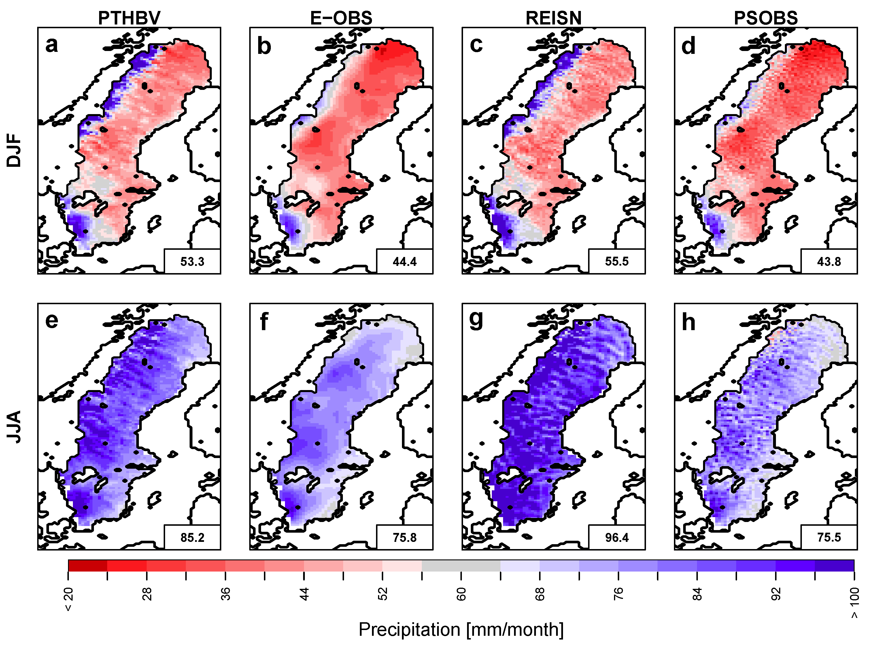
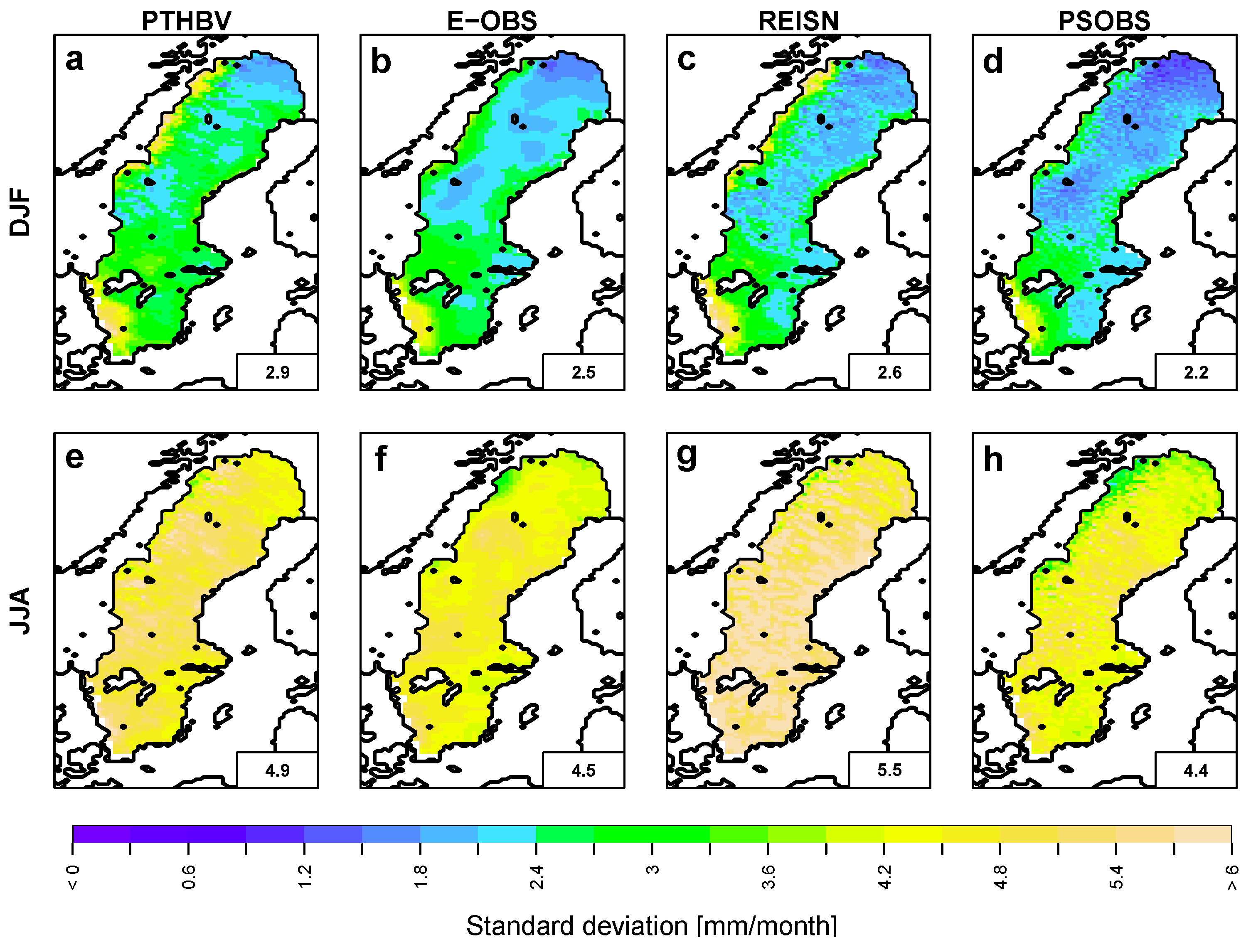
5.2. Evaluation


5.3. Bias Correction


6. Discussion
7. Conclusions
Acknowledgments
Author Contributions
Conflicts of Interest
References
- Haylock, M.; Hofstra, N.; Tank, A.M.G.K.; Klok, E.J.; Jones, P.D.; New, M. A European daily high-resolution gridded dataset of surface temperature, precipitation and sea-level pressure. J. Geophys. Res. 2008, 113. [Google Scholar] [CrossRef]
- Graham, L.; Andréasson, J.; Carlsson, B. Assessing climate change impacts on hydrology from an ensemble of regional climate models, model scales and linking methods—A case study on the Lule river basin. Clim. Chang. 2007, 81, 293–307. [Google Scholar] [CrossRef]
- Piani, C.; Haerter, J.O.; Coppola, E. Statistical bias correction for daily precipitation in regional climate models over Europe. Theor. Appl. Climatol. 2010, 99, 187–192. [Google Scholar] [CrossRef]
- Berg, P.; Feldmann, H.; Panitz, H.J. Bias correction of high resolution regional climate model data. J. Hydrol. 2012, 448–449, 80–92. [Google Scholar] [CrossRef]
- Johansson, B.; Chen, D. The influence of wind and topography on precipitation distribution in Sweden: Statistical analysis and modelling. Int. J. Climatol. 2003, 23, 1523–1535. [Google Scholar] [CrossRef]
- Weedon, G.; Gomes, S.; Viterbo, P.; Shuttleworth, W.; Blyth, E.; Österle, H.; Adam, C.; Bellouin, N.; Boucher, O.; Best, M. Creation of the watch forcing data and its use to assess global and regional reference crop evaporation over land during the twentieth century. J. Hydrometeor. 2011, 12, 823–848. [Google Scholar] [CrossRef]
- Samuelsson, P.; Jones, C.; Willén, U.; Ullerstig, A.; Gollvik, S.; Hansson, U.; Jansson, C.; Kjällström, E.; Nikulin, G.; Wyser, K. The Rossby Centre regional climate model RCA3: Model description and performance. Tellus 2011, 63A, 4–23. [Google Scholar] [CrossRef]
- Berg, P.; Döscher, R.; Koenigk, T. Impacts of using spectral nudging on regional climate model RCA4 simulations of the Arctic. Geosci. Model Dev. 2013, 6, 849–859. [Google Scholar] [CrossRef]
- Von Storch, H.; Langenberg, H.; Feser, F. A spectral nudging technique for dynamical downscaling purposes. Mon. Weather Rev. 2000, 128, 3664–3673. [Google Scholar] [CrossRef]
- Dee, D.P.; Uppala, S.M.; Simmons, A.J.; Berrisford, P.; Poli, P.; Kobayashi, S.; Andrae, U.; Balmaseda, M.A.; Balsamo, G.; Bauer, P.; et al. The ERA-Interim reanalysis: Configuration and performance of the data assimilation system. Q. J. R. Meteorol. Soc. 2011, 137, 553–597. [Google Scholar] [CrossRef]
- Hazeleger, W.; Wang, X.; Severijns, C.; S¸tefaănescu, S.; Bintanja, R.; Sterl, A.; Wyser, K.; Semmler, T.; Yang, S.; van den Hurk, B.; et al. EC-Earth V2. 2: Description and validation of a new seamless earth system prediction model. Clim. Dyn. 2012, 39, 2611–2629. [Google Scholar] [CrossRef]
- Koenigk, T.; Brodeau, L. Ocean heat transport into the Arctic in the twentieth and twenty-first century in EC-Earth. Clim. Dyn. 2013, 42, 3101–3120. [Google Scholar] [CrossRef]
- Koenigk, T.; Brodeau, L.; Graversen, R.G.; Karlsson, J.; Svensson, G.; Tjernström, M.; Willen, U.; Wyser, K. Arctic climate change in 21st century CMIP5 simulations with EC-Earth. Clim. Dyn. 2013, 40, 1–25. [Google Scholar] [CrossRef]
- Lucas-Picher, P.; Boberg, F.; Christensen, J.H.; Berg, P. Dynamical downscaling with reinitializations: A method to generate finescale climate datasets suitable for impact studies. J. Hydrometeorol. 2013, 14, 1159–1174. [Google Scholar] [CrossRef]
- Yang, W.; Andréasson, J.; Graham, L.P.; Olsson, J.; Rosberg, J.; Wetterhall, F. Distribution based scaling to improve usability of regional climate model projections for hydrological climate change impacts studies. Hydrol. Res. 2010, 41, 211–229. [Google Scholar] [CrossRef]
- Buser, C.M.; Künsch, H.R.; Lüthi, D.; Wild, M.; Schär, C. Bayesian multi-model projection of climate: Bias assumptions and interannual variability. Clim. Dyn. 2009, 33, 849–868. [Google Scholar] [CrossRef]
- Haerter, J.O.; Hagemann, S.; Moseley, C.; Piani, C. Climate model bias correction and the role of timescales. Hydrol. Earth Syst. Sci. 2011, 15, 1065–1079. [Google Scholar] [CrossRef]
- Taylor, K.E. Summarizing multiple aspects of model performance in a single diagram. J. Geophys. Res. 2001, 106, 7183–7192. [Google Scholar] [CrossRef]
© 2015 by the authors; licensee MDPI, Basel, Switzerland. This article is an open access article distributed under the terms and conditions of the Creative Commons Attribution license (http://creativecommons.org/licenses/by/4.0/).
Share and Cite
Berg, P.; Bosshard, T.; Yang, W. Model Consistent Pseudo-Observations of Precipitation and Their Use for Bias Correcting Regional Climate Models. Climate 2015, 3, 118-132. https://doi.org/10.3390/cli3010118
Berg P, Bosshard T, Yang W. Model Consistent Pseudo-Observations of Precipitation and Their Use for Bias Correcting Regional Climate Models. Climate. 2015; 3(1):118-132. https://doi.org/10.3390/cli3010118
Chicago/Turabian StyleBerg, Peter, Thomas Bosshard, and Wei Yang. 2015. "Model Consistent Pseudo-Observations of Precipitation and Their Use for Bias Correcting Regional Climate Models" Climate 3, no. 1: 118-132. https://doi.org/10.3390/cli3010118