Perspectives for Very High-Resolution Climate Simulations with Nested Models: Illustration of Potential in Simulating St. Lawrence River Valley Channelling Winds with the Fifth-Generation Canadian Regional Climate Model

Abstract

With the refinement of grid meshes in regional climate models permitted by the increase in computing power, the grid telescoping or cascade method, already used in numerical weather prediction, can be applied to achieve very high-resolution climate simulations. The purpose of this study is two-fold: (1) to illustrate the perspectives offered by climate simulations on kilometer-scale grid meshes using the wind characteristics in the St. Lawrence River Valley (SLRV) as the test-bench; and (2) to establish some constraints to be satisfied for the physical realism and the computational affordability of these simulations. The cascade method is illustrated using a suite of five one-way nested, time-slice simulations carried out with the fifth-generation Canadian Regional Climate Model, with grid meshes varying from roughly 81 km, successively to 27, 9, 3 and finally 1 km, over domains centered on the SLRV. The results show the added value afforded by very high-resolution meshes for a realistic simulation of the SLRV winds. Kinetic energy spectra are used to document the spin-up time and the effective resolution of the simulations as a function of their grid meshes. A pragmatic consideration is developed arguing that kilometer-scale simulations could be achieved at a reasonable computational cost with time-slice simulations of high impact climate events. This study lends confidence to the idea that climate simulations and projections at kilometer-scale could soon become operationally feasible, thus offering interesting perspectives for resolving features that are currently out of reach with coarser-mesh models.

1. Introduction

Today’s general circulation models (GCMs), also known has global climate models, have proven their reliability at reproducing past and present climates, and they constitute the primary tools for making projections of future climate consequent to anthropogenic effects [1]. Owing to their humongous computational cost, resulting from the combination of their complex formulation, the time to achieve dynamic equilibrium with multi-century long integrations and the need to establish statistical significance with ensemble simulations, operational GCMs are forced to employ a rather coarse resolution. The average grid spacing of today’s GCMs participating in the AR5 report on century-scale climate projections is about 300 km [2]. Such horizontal resolutions are too coarse to satisfy the needs of most climate-change impact studies [3,4,5]. Given that the computational cost of a GCM is inversely proportional to the third or fourth power of the grid spacing (as discussed in detail in Section 4), reducing the grid spacing of GCMs is prohibitive for long simulations, because of insufficient computational resources available to most research centers.

An alternative approach to coarse GCMs was proposed in the late 1980s: nested regional climate models (RCMs) [6,7], known in numerical weather prediction (NWP) as limited-area models (LAMs). Based on the concept of dynamical downscaling [8], the computational domain is restricted to a study region (typically the size of a continent or smaller), and the lateral boundary conditions (LBCs) are provided either by reanalyses or GCM simulations/projections. One must however recognize that regional climate modeling is critically dependent on the fidelity of the LBCs at large scales; nonetheless, examining the sensitivity of local-scale phenomena to changes in GCM-simulated large-scale conditions has proven to be a worthwhile approach. Over the past two decades, RCMs have become sophisticated tools for present-day simulations and future climate projections. Over time, several improvements have been made in the formulation of RCMs: the grid meshes have been refined; the computational domains have enlarged; and the simulated periods have lengthened. For example, while initially, typical domains contained about 50 by 50 grid points and simulation periods seldom exceeded one month (e.g., [7]), nowadays RCMs are regularly integrated over domains of 200 by 200 grid points and simulated periods extend to centuries, as, for example, in the Coordinated Regional Climate Downscaling Experiment (CORDEX) [9,10] initiated in 2009. Spatial resolution, however, has been rather slow to evolve from the initial grid meshes of about 60 km. Indeed, the standard CORDEX experiment calls for grid meshes of 0.44° (~50 km), although groups that can afford it are also encouraged to use grid meshes of 0.11° (~12 km). Some groups have since performed extensive simulations with 12-km grid meshes (e.g., [11,12,13,14,15]), although such simulations remain extremely costly when performed over large regions, such as over entire continents.

With a grid spacing of a few tens of km, some interesting mesoscale processes begin to be partly resolved by the models. However, such a resolution is still too coarse for the proper representation of several important weather processes and climate features that may be relevant for high-impact weather studies. The simulation of phenomena, such as downslope windstorms in the lee of large mountains, wind channelling in valleys, lake/sea breezes, katabatic winds, mesoscale convective complexes, mixed precipitation events, to name but a few, requires using much finer meshes to resolve the underlying physical processes explicitly. The non-hydrostatic dynamical core of some LAMs allows convection-permitting simulations using grid spacing smaller than 10 km (e.g., [16,17,18,19]). Recently a flurry of activities has been initiated in several groups around the world towards the use of kilometer-scale RCM simulations (e.g., [11,12,13,20,21,22,23,24,25]); several of these have been reported in the proceedings of the 3rd Lund Regional-scale Climate Modeling Workshop held in Sweden [26].

As computing power continues to increase, the use of very fine meshes of a few km for climate modeling on limited domains will gradually become feasible for more groups. The large resolution jump between the kilometer-mesh RCM and the coarse-mesh LBCs from GCM would however imply the requirement of using very large regional domains, of order of thousands of grid points in the linear dimension, in order to allow sufficient room for the spin-up of fine scales. Based on the rule-of-thumb that the regional domain of a nested model should comprise a minimum of 20 grid points of the driving model in the linear dimension [27], we estimate that a 1-km mesh RCM driven by a 300-km mesh GCM would hence need a domain of about 6000 × 6000 grid points. Such domains would be prohibitively expensive computationally for simulations on climate time scales. This provides the motivation for seeking efficient ways to produce much higher resolution climate simulations and projections at an affordable computational expense. An alternative approach to direct dynamical downscaling is the use of telescoping domains, also called the cascade method. In this case, the resolution jump between each simulation in the cascade is under the control of the user, thus allowing the use of more limited domains at each step of the cascade, with a resulting associated appreciable computational savings. The cascade has already been employed for quite some time in NWP (e.g., [28,29,30]). It consists in a suite of nested-grid simulations, with larger domain coarse-mesh simulations successively providing the LBCs for smaller domain simulations on finer meshes. Although the grid telescoping method has been used in NWP and for mesoscale case studies, it has only recently started being used for climate applications. Despite significant remaining challenges, these studies lend interesting perspectives for the application of the grid telescoping cascade method to achieve very high-resolution climate simulations and projections.

Most of the aforementioned work investigating the added value of kilometer-scale climate simulations focused on intense precipitations, some in connection with major topographic forcing. This paper takes a rather different perspective by looking at a phenomenon of dynamical origin and associated with rather modest topographical features: that of wind channelling in the St. Lawrence River Valley (SLRV; see Figure 1 for topographical features). This study will investigate the impact of dynamical downscaling on the simulation of wind channelling in the SLRV to determine the minimum resolution required for an appropriate reproduction of the climatological signature of the SLRV winds. SLRV wind channelling is an important local process, especially in winter and spring seasons, as it can produce a very strong temperature inversion in lower layers of the atmosphere, which, combined with the associated warm front precipitation, can lead to important freezing rain events and a large amount of icing at the surface [31]. The SLRV’s winds are a crucial element of local climate, and damages caused by freezing rain events can produce important societal and economic impacts. Whether changes in the frequency and occurrence of such events could result from the anticipated anthropogenic climate change is an important issue, which we hope could be advantageously explored with the cascade methodology.

Figure 1. Geographical details of the study domain. The St. Lawrence River Valley (SLRV), Lake Champlain Valley (LCV), Lake Ontario and the Laurentian, Appalachian, Adirondack, Green and White mountains are indicated. The red and blue dots indicate the locations of Montréal and Québec City, respectively. Topographic height (meters) is shown by grey tones.

Figure 1. Geographical details of the study domain. The St. Lawrence River Valley (SLRV), Lake Champlain Valley (LCV), Lake Ontario and the Laurentian, Appalachian, Adirondack, Green and White mountains are indicated. The red and blue dots indicate the locations of Montréal and Québec City, respectively. Topographic height (meters) is shown by grey tones.

The paper is organized as follows. The experimental design of simulations performed with the fifth-generation Canadian Regional Climate Model (CRCM5) on a series of telescoping domains with meshes varying from roughly 81 km, successively to 27, 9, 3 and, finally, 1 km, are described in Section 2. The spin up of fine scales is studied in Section 3 to determine the time required to reach dynamical equilibrium at each step of the cascade. This is addressed with the study of kinetic energy spectra over different domains and as a function of time to establish some constraints for physical realism and proper interpretation of cascade simulations (Section 3.1). The results are also analyzed in terms of resolved SLRV topographical winds as a function of the different horizontal resolution (Section 3.2). Finally, to look forward, a suggestion of using an event-based time-slice approach to limit computational cost at its minimum is proposed in Section 4, which, in principle, would allow performing very high-resolution climate simulations at quite an affordable computational cost. Section 5 summarizes and provides some conclusions.

2. Experimental Design

2.1. The Model Description

The experiments have been performed with the fifth-generation Canadian RCM (CRCM5; [32,33,34]). CRCM5 is based, in large part, on the Global Environmental Multiscale model (GEM; [35,36]) developed by Environment Canada for NWP. The dynamical core uses a two-time-level quasi-implicit semi-Lagrangian marching scheme, and the horizontal discretization is based on an Arakawa staggered C-grid. The model has a fully elastic non-hydrostatic option [37], in which case the vertical coordinate is terrain-following hydrostatic pressure [38]. In CRCM5, a sponge zone [39] of ten grid points is applied around the perimeter of the regional domain where the inner solution is gradually blended with the outer solution imposed as LBCs.

The land-surface processes are formulated following the most recent version of the Canadian Land Surface Scheme (CLASS 3.5; [40,41]) that allows for a detailed representation of vegetation, land-surface types, organic soil and a flexible number of layers. Most other subgrid-scale physical parameterization modules have been taken from GEM as used for NWP: correlated-K terrestrial and solar radiation schemes [42], turbulent kinetic energy closure planetary boundary layer and vertical diffusion [43,44,45], boundary-layer clouds [43,46], shallow-convection clouds [47,48] and a weak ∇⁶ lateral diffusion.

The subgrid-scale physical parameterizations, as the name indicates, aim at representing the ensemble effect of physical processes operating below the resolved scales in models. Although the parameterizations ought clearly to vary as a function of the model’s mesh, it is often difficult to develop robust formulations that self-adjust to model resolution. In particular, a distinct challenge to atmospheric modeling with horizontal grid spacing around 10 km is the transition from fully parameterized to fully resolved deep convection in the so-called “grey zone” [12,49,50,51,52,53,54], where deep convection is partly resolved and partly a subgrid-scale process. For the experiments reported below, moist convection, cloud microphysics and subgrid-scale orographic effects were adjusted depending on resolution. Simulations with grid meshes coarser than about 10 km were performed with the hydrostatic dynamical core, and the Sundqvist diagnostic condensation scheme [55] was used for stratiform clouds and large-scale precipitation, with precipitation type diagnosed via an empirical algorithm developed by Bourgouin [56]. The Kain and Fritsch deep-convection scheme [57] is employed, and the subgrid-scale orographic effects are parameterized following the McFarlane mountain gravity-wave drag [58] and the low-level orographic blocking schemes of [59]. Simulations with grid meshes finer than 10 km were performed with the non-hydrostatic dynamical core, using the Milbrandt and Yau double-moment bulk-microphysics scheme [60,61] that provides detailed information on the different types of precipitation (snow, rain, graupel and hail), and parameterizations of deep convection and subgrid-scale orographic effects were then turned off. In the simulations, sea surface temperatures, sea-ice concentration and resolved lakes are prescribed from ERA-Interim reanalyses [62].

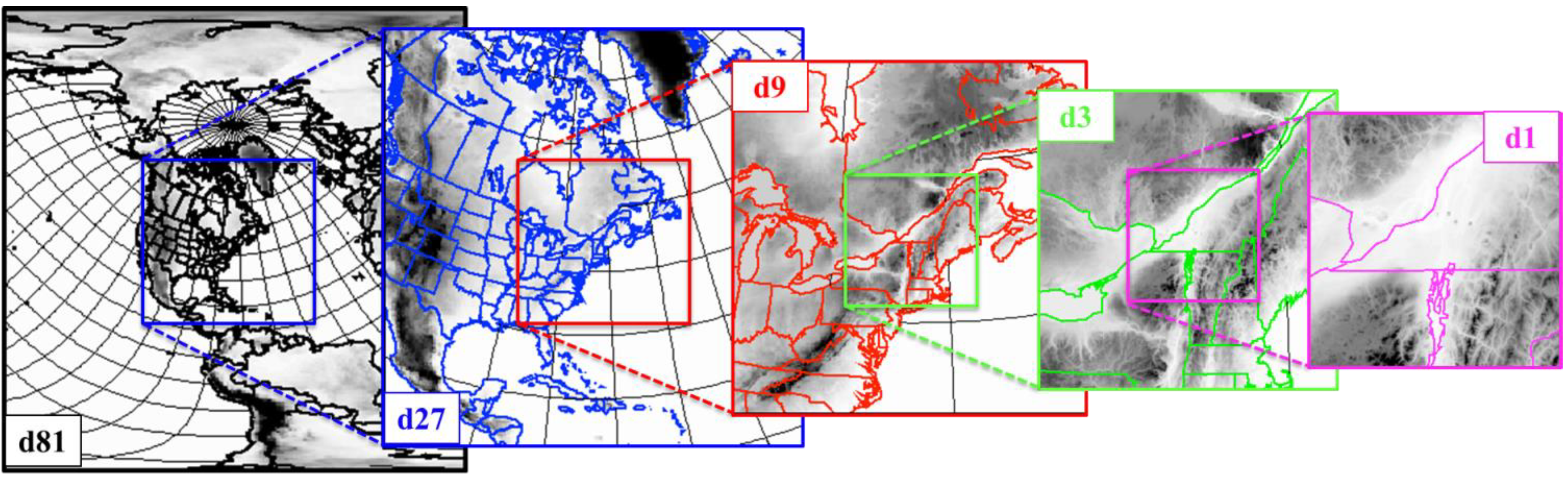
2.2. The Cascade Description

A suite of five one-way nested CRCM5 simulations has been performed with horizontal grid meshes of 0.81°, 0.27°, 0.09°, 0.03° and 0.01° (hereinafter referred to as d81, d27, d9, d3 and d1, respectively), using a factor of three in mesh size between each stage in the cascade. The domains are centered over Montréal, Canada (45°30ʹN, 73°35ʹW), as shown in Figure 2. The domains are square with roughly the same number of grid points in the horizontal. The computational domains comprise 220 × 220 grid points for the d81 simulation and 245 × 245 grid points for the other simulations; this corresponds to the following free domains (excluding the Davies’ sponge zone) of 200 × 200 grid points for the d81 simulation and 225 × 225 grid points for the other simulations. Each fine-mesh domain in centered in the middle third of the driving coarser mesh domain, in such a way as to provide ample room for the spin-up of fine scales at the resolution jump between each domain. As shown in Figure 2, the model-resolved topographical features become more detailed with finer meshes; indeed, it can be seen that some mountain peaks’ heights have been doubled from the d81 to the d3 simulations. Hence, the influence of the surrounding SLRV topography is expected to improve in higher resolution simulations.

Figure 2. The computational domains used for the fifth-generation Canadian Regional Climate Model (CRCM5) cascade: d81 (0.81°; black), d27 (blue), d9 (red), d3 (green) and d1 (magenta) simulations. The domains are square and centered on Montréal (Québec, Canada). The grey tones represent the topography definition in each domain (see the legend of Figure 1).

Figure 2. The computational domains used for the fifth-generation Canadian Regional Climate Model (CRCM5) cascade: d81 (0.81°; black), d27 (blue), d9 (red), d3 (green) and d1 (magenta) simulations. The domains are square and centered on Montréal (Québec, Canada). The grey tones represent the topography definition in each domain (see the legend of Figure 1).

All simulations used 56 levels in the vertical, with a top computational level at 10 hPa. The time steps were adjusted to maintain roughly the same Courant numbers: 30 min, 10 min, 200 s, 60 s and 20 s are used for the d81, d27, d9, d3 and d1 simulations, respectively. The d81 simulation was driven at 6-hourly intervals by the ERA-Interim data, available to us on a 2° mesh. The archival time intervals were adapted as a function of grid mesh in order to provide suitable LBCs driving data for the next model in the cascade. The d81 simulation was archived at 3-h intervals to provide the LBCs for the d27; the d27 simulation provided the LBCs for the d9 simulation at hourly intervals; the d9 simulation provided the LBCs for d3 at 20-min intervals; and the d3 simulation provided the LBC for the d1 simulation at 5-min intervals. As mentioned earlier, a major change of formulation was operated in CRCM5 around 10 km, with finer grid meshes being considered as convection-permitting. Two d9 simulations were performed, one using large-scale parameterizations and the other using fine-scale parameterizations; the latter provided LBCs fields for hydrometeors as required by the Milbrandt and Yau microphysics scheme [60,61] used with finer meshes.

Section 4 will discuss in greater detail the interest of grid telescoping for climate-scale simulations. For this feasibility study without any pretense of statistical significance, only short simulations were performed. The launching date of higher resolution simulations in the cascade was delayed to allow for spin-up, and the simulation lengths were reduced with increased resolution in order to reduce computational cost: 6 months for d81 (from 1 October 2001 to 1 April 2002), 4 months for d27 (from 1 December 2001 to 1 April 2002), 3 months for d9 (from 1 January to 1 April 2002), 1 month for d3 (from 4 February to 7 March 2002) and 15 days for d1 (from 12 February to 1 March 2002).

3. Results

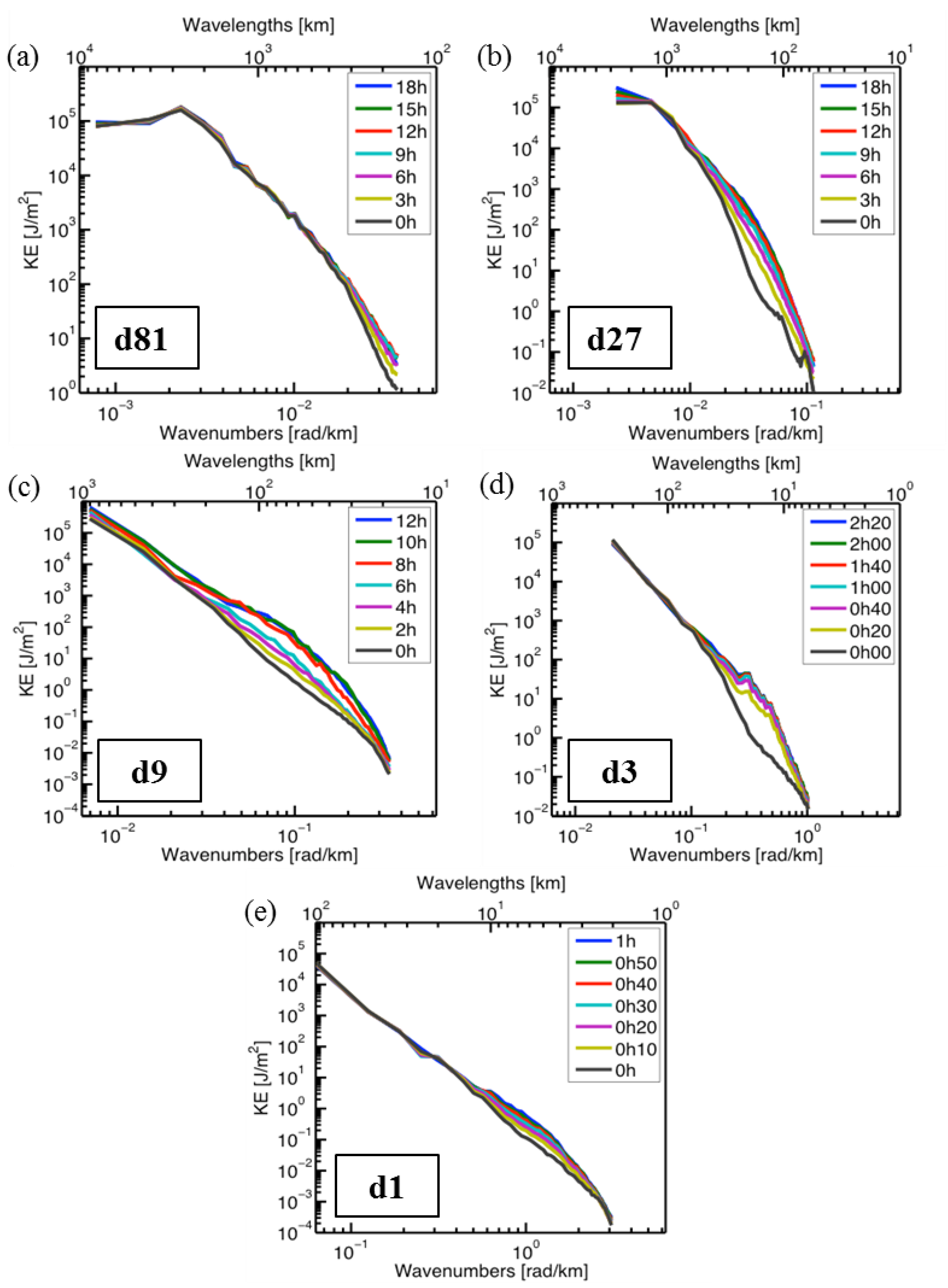
3.1. Kinetic Energy Spectra

Kinetic energy (KE) spectra have been useful to characterize the atmospheric dynamics in global analyses and simulations (e.g., [63,64]). Because models solve discretized versions of the field equations, an important issue with any numerical model is their effective resolution (e.g., [65]). An additional consideration with nested LAM is the spin-up time required to develop fine scales when initialized and driven by low-resolution data (e.g., [66]). The spin-up time needs to be properly dealt with when time-slice simulations are considered as opposed to continuous ones. Variance spectra are useful tools to address such issues, allowing one to quantify how much power there is in different spatial scales of simulated atmospheric fields at various times. At synoptic scales, where the quasi-geostrophic equilibrium prevails, theories and analyses show that the KE spectrum follows a k⁻³ power law, with k the horizontal wavenumber (e.g., [67,68]). Several studies indicate a transition to a spectral slope of k^−5/3 at the mesoscale (e.g., [69,70]); the theories explaining this part of the spectrum are not well understood, however, nor at what scale the transition between the two spectral slopes occurs.

KE spectra can be computed over a limited-area domain using the discrete cosine transform (DCT; [71]). The variances of the horizontal wind components, σ_U²(k) and σ_V²(k), are computed on pressure levels with the DCT as a function of the two-dimensional wavenumber k and then combined to form the KE spectrum ${\mathrm{\sigma }}_{\mathrm{K}\mathrm{E}}^2\left(\mathrm{k}\right)=\frac{{\mathrm{\sigma }}_{\mathrm{U}}^2(\mathrm{k})+{\mathrm{\sigma }}_{\mathrm{V}}^2(\mathrm{k})}{2}$, which can then be vertically integrated over some atmospheric depth and temporally averaged over some selected period. KE spectra of the various CRCM5 simulations have been computed and will be analyzed to study the spin-up process and the effective resolution of each simulation in the cascade.

3.1.1. Spin-Up Time

Starting from and driven by coarse-mesh data, high-resolution models are known to develop their own fine-scale variance (e.g., [67]). Figure 3 confirms this result by showing KE spectra at various times in the cascade simulations. To reduce spurious effects caused by the lateral boundaries, the spectra were computed over the 50 × 50 inner grid points of each computational domain. In Figure 3, all axes are logarithmic. The ordinate corresponds to the ${\mathrm{\sigma }}_{KE}^2\left(k\right)$ (in J/m²), vertically integrated from 700 to 200 hPa; the upper abscissa indicates the wavelengths λ (in km) and the lower abscissa the wavenumbers k = 2π/λ (in radians km⁻¹). With the DCT, the shortest wavelength or Nyquist length scale is twice the grid spacing (2 × ∆x), and the longest wavelength is twice the domain size (i.e., the number of grid points multiplied by the grid spacing, 2 × 50 × ∆x). The different line colors correspond to different times in the simulations.

The results indicate that fine-scale KE develops from larger scale initial and lateral boundary conditions, and after some initial growth period, the curves converge to their asymptotic values. The spin-up time appears to be shorter with finer meshes, varying from roughly 12 h for d81 and d27, 10 h for d9, 2 h for d3 and 50 min for d1. These results are in general agreement with those obtained by Skamarock [72] with the Weather Research Forecasting (WRF) model over the USA for three days in June, 2003: he obtained spin-up times in the range of 6 and 12 h for simulations with grid spacing of 4, 10 and 22 km. The spin-up time is an important consideration in the design of time-slice telescoping-grid simulations: it is necessary to leave some time at each stage in the cascade for the higher resolution simulations to spin-up small scales from coarse-scale initial and lateral boundary conditions. The above analysis only concerned atmospheric dynamics spin-up. In practice, the adjustment of land-surface processes also needs to be considered; these adjustment times may be substantially longer than those for the atmosphere.

Figure 3. Kinetic energy (KE) spectra at various times after the launching of the (a) d81, (b) d27, (c) d9, (d) d3 and (e) d1 simulations. The different line colors correspond to different times in the simulation, as identified by the respective panels’ legends. The ordinates are the KE (J/m²) vertically averaged from 700 to 200 hPa; the upper abscissas represent the wavelengths (km) and the lower abscissas the wavenumbers (rad/km). All axes are shown on logarithmic scales.

Figure 3. Kinetic energy (KE) spectra at various times after the launching of the (a) d81, (b) d27, (c) d9, (d) d3 and (e) d1 simulations. The different line colors correspond to different times in the simulation, as identified by the respective panels’ legends. The ordinates are the KE (J/m²) vertically averaged from 700 to 200 hPa; the upper abscissas represent the wavelengths (km) and the lower abscissas the wavenumbers (rad/km). All axes are shown on logarithmic scales.

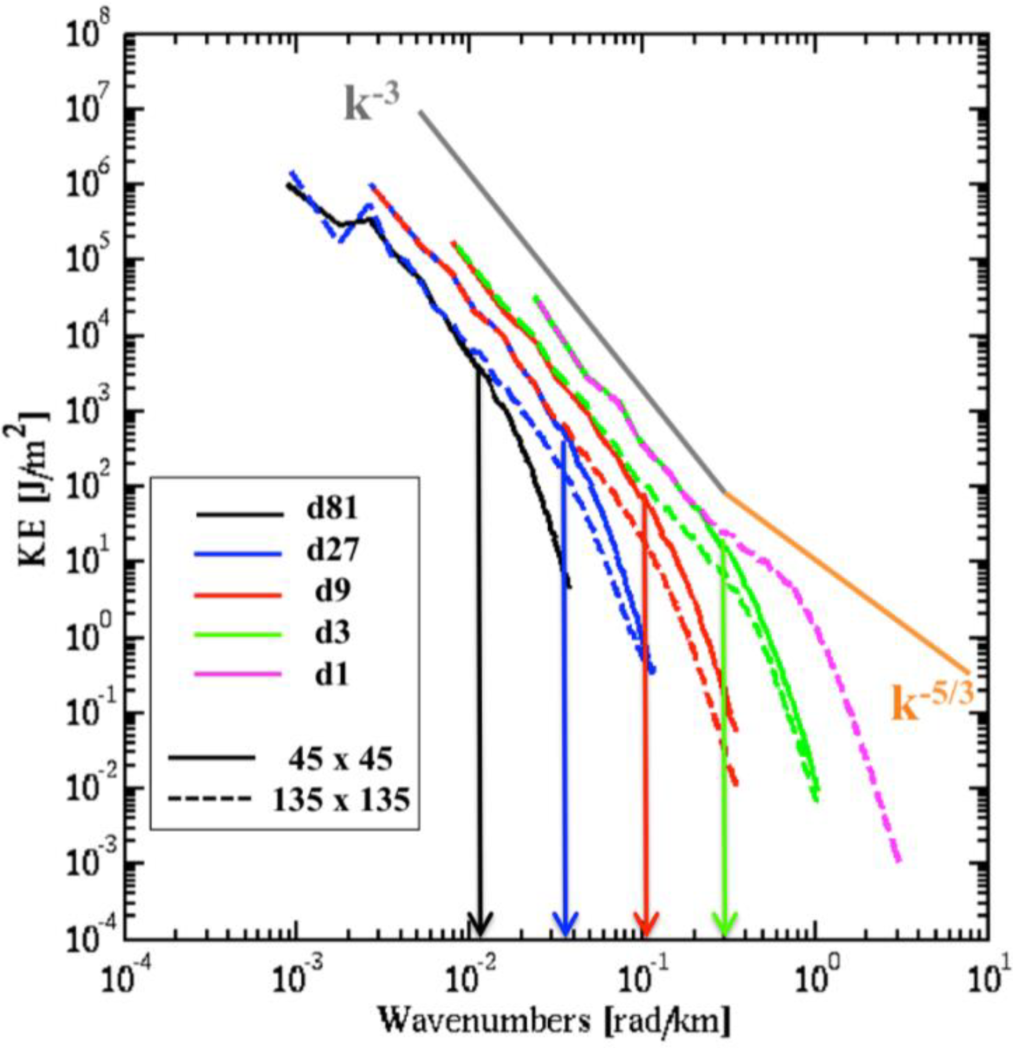
3.1.2. Effective Resolution

While the shortest permitted wavelength in a simulation is the Nyquist length scale, equal to twice the grid spacing by virtue of the properties of Fourier series, it is important to realize that permitted length scales are not equally well resolved in numerical models and, hence, distinguishing the effective resolution of a model from its mesh size is needed (e.g., [72,73]). Variance spectra provide a first measure of the necessary condition to be fulfilled for declaring a scale as resolved; the actual simulation skill is a further condition, but this will not be considered in the following. The shape of KE spectra near the upper wavenumber limit of a model provides useful information on the influence of model numerical techniques and dissipation mechanisms. The role of dissipation in particular is to prevent small-scale variance from piling up near the shortest permitted scale, thus causing aliasing that would misrepresent the physical interactions [74]. Hence, while insufficient dissipation will result in a raised spectrum tail, excessive dissipation will cause over-damping of the spectrum’s tail (e.g., [75]). A pragmatic definition of the effective resolution of a model is the length scale at which a spectrum begins to exhibit damping relative to some reference spectrum obtained from either theory, an observational dataset or from a finer mesh simulation. Length scales shorter than the effective resolution thus defined have to be considered as suspect in model simulations.

Figure 4 shows KE spectra of the five simulations in the cascade, averaged vertically from 700 to 200 hPa and temporally from 0000 UTC 13 February to 0000 UTC 1 March 2002 in the common period, excluding the first 24 h of integration for spin-up. Because limited-area spectral variances vary with domain size, two computed spectra are shown for each simulation: the solid lines show spectra computed over 45 × 45 grid-point domains and the dashed lines show spectra computed over larger 135 × 135 grid-point domains. This way, the solid line of a d_{3 × n} coarser mesh simulation can be compared to the dashed line of the d_n finer mesh simulation, with n ∈ {1, 3, 9, 27}, as these are computed over the same physical region, to define the effective resolution of a simulation using the nearest finer resolution spectrum as the reference.

The dropping tails of the kinetic energy spectrum at high wavenumbers signals the effect of the dissipation of energy near the finest permitted scales on the model grid. When the spectra of two simulations performed on different grid meshes are compared, the wavenumber where the two simulations diverge represent the scale where the coarser resolution begins to be dynamically suspect because of the effect of excessive numerical dissipation. The subjectively-estimated effective resolution wavenumbers, indicated in Figure 4 by colored arrows, are approximately 0.011, 0.033, 0.1 and 0.3 rad km⁻¹ for d81, d27, d9 and d3 simulations, respectively. This gives effective resolution wavelengths (λ_eff) of roughly 571, 190, 63 and 21 km, which correspond to roughly seven-times the grid spacing, i.e., 3.5 × (2 × ∆x). This finding is consistent with the numerical results obtained by Skamarock [72] for grid meshes of 22, 10 and 4 km and with numerical analysis theory that estimates the effective resolution of low-order finite-difference schemes to lie between 6 × ∆x and 10 × ∆x (e.g., [72]). Figure 4 also shows a shift in the spectral slopes from k⁻³ at large scales to k^−5/3 at small scales in the d1 simulation. The transition occurs near k = 0.31 rad∙km⁻¹, corresponding approximately to λ = 20 km. This value however needs to be taken with reservations, as it occurs close to the effective resolution of 7 km.

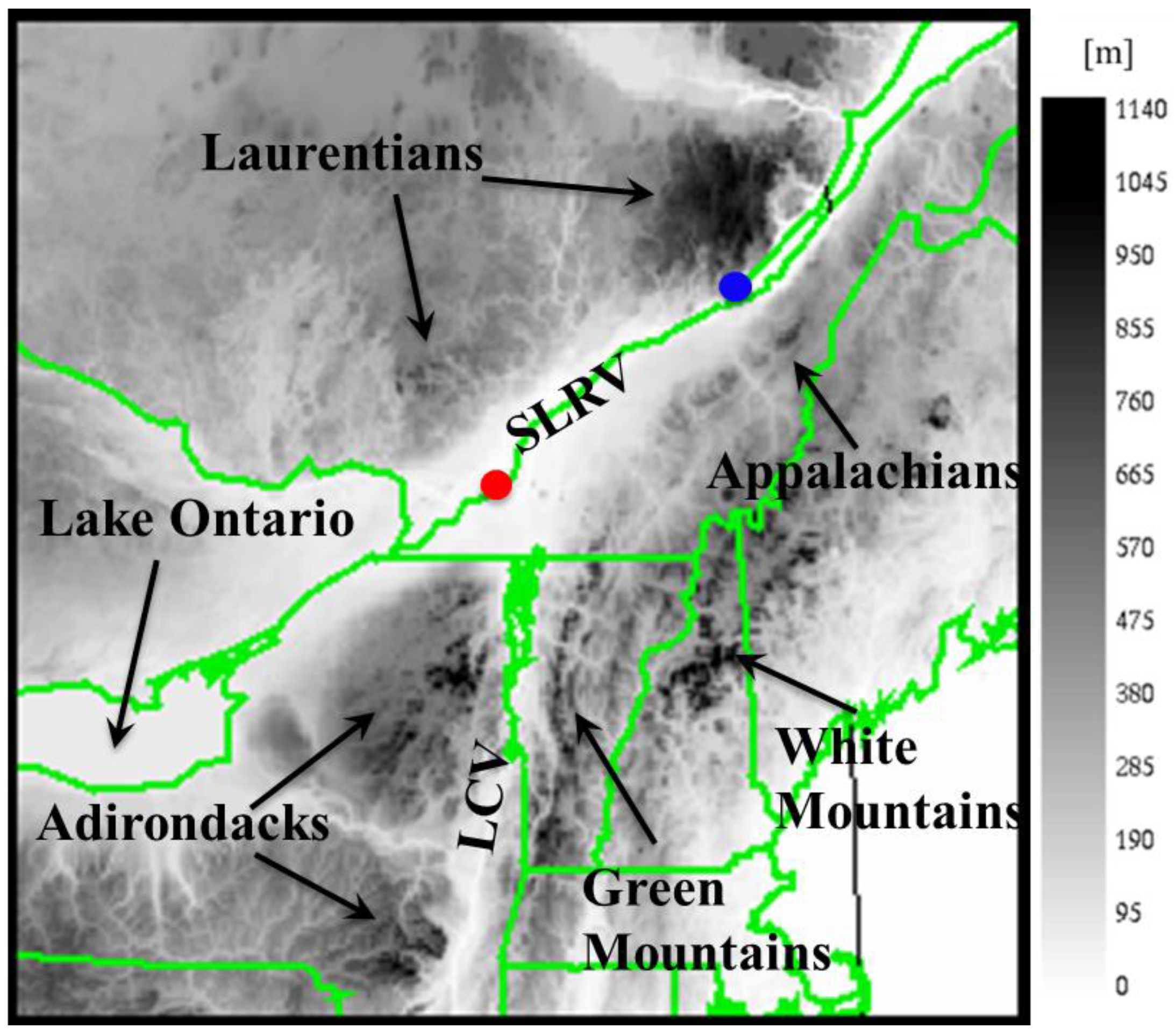
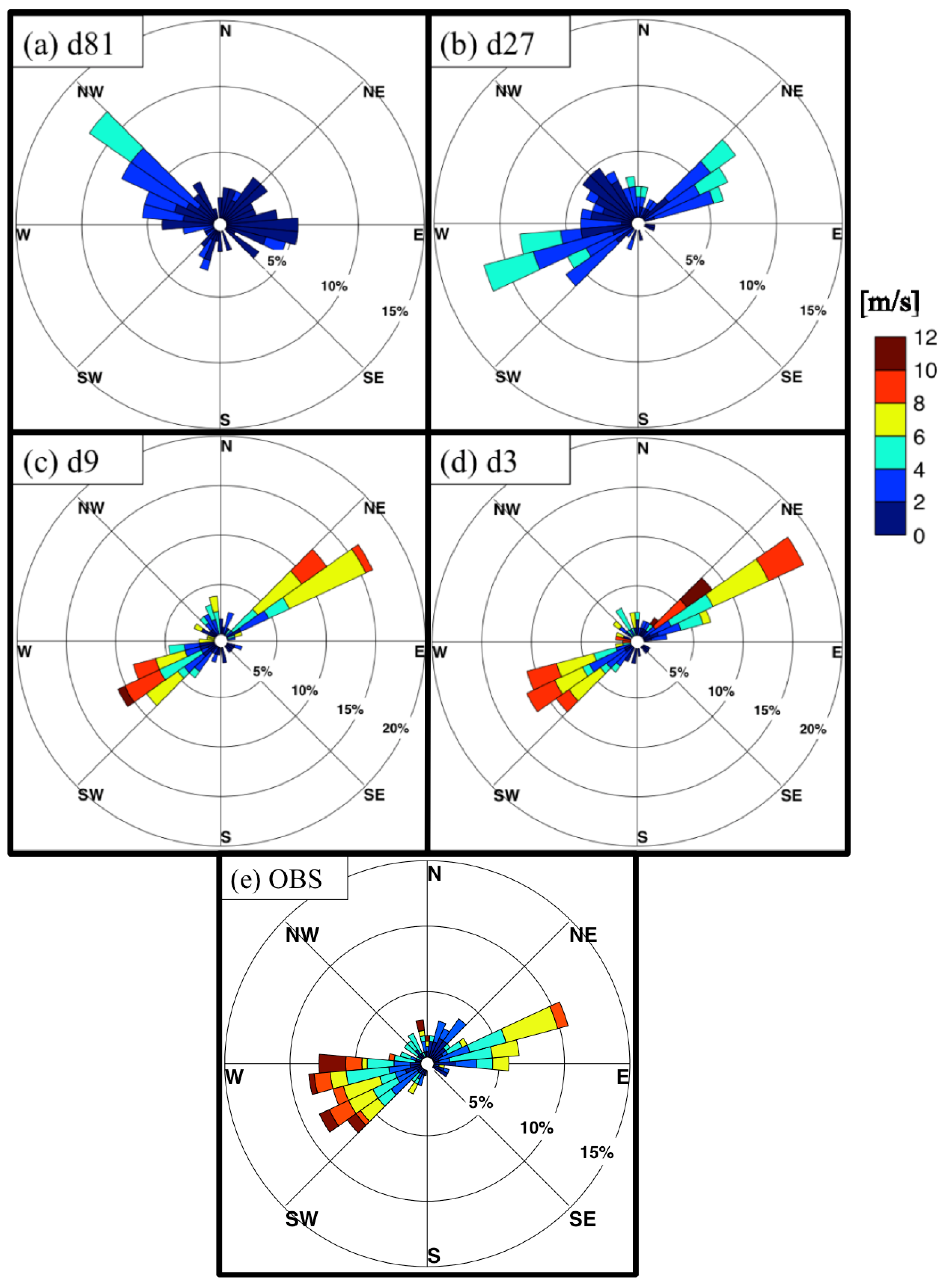
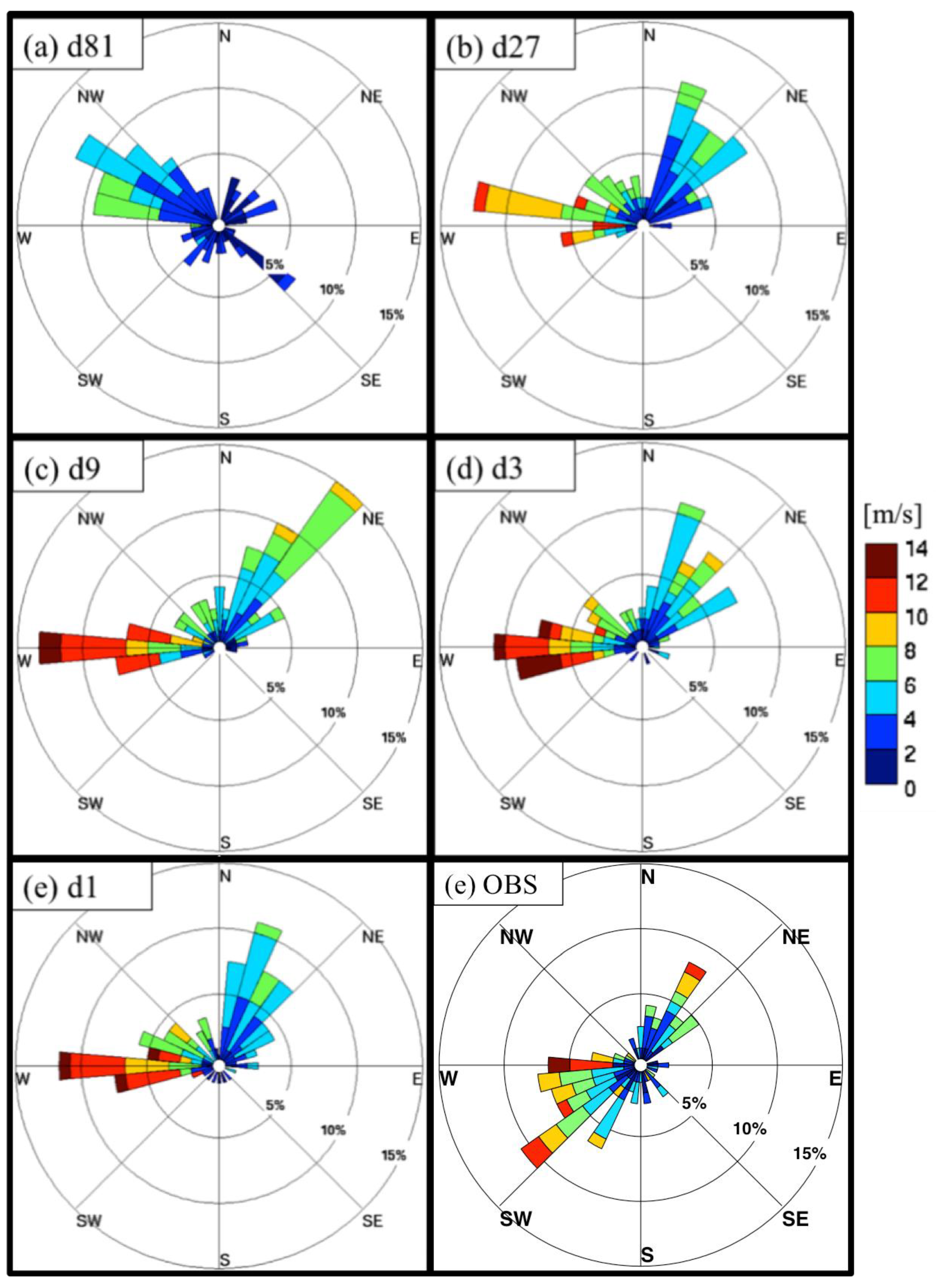
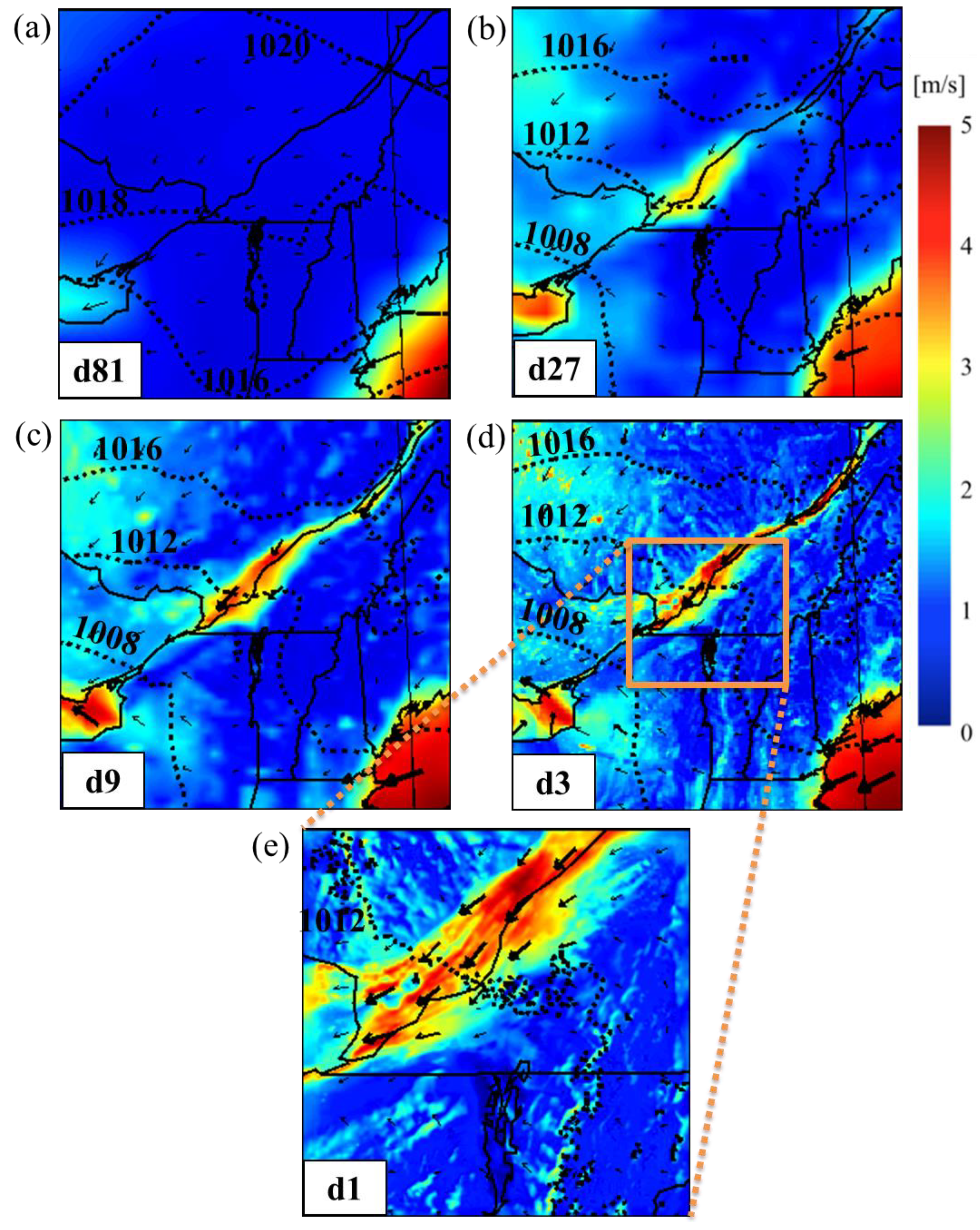
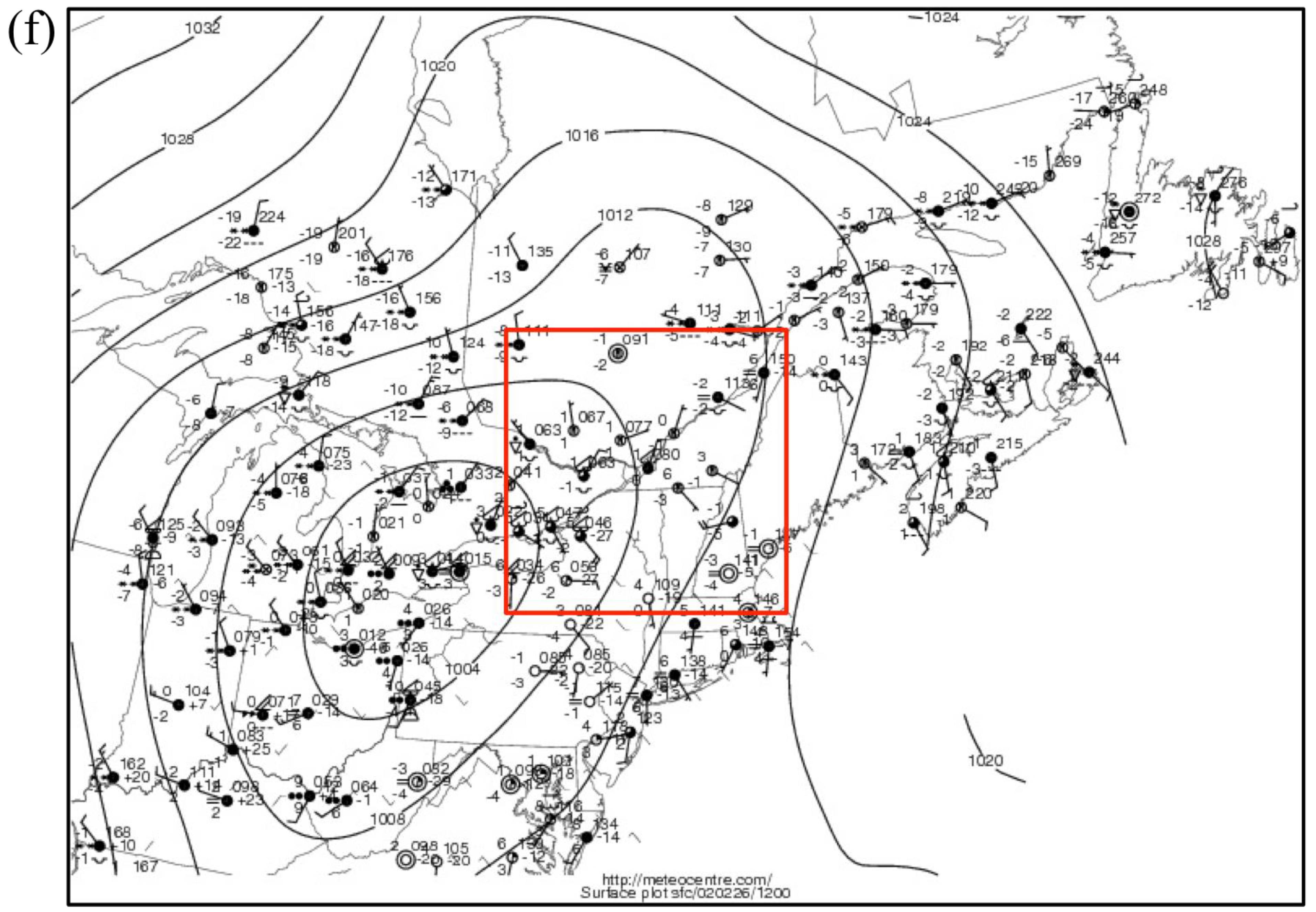
3.2. St. Lawrence River Valley Features

As mentioned before, wind channelling represents an important local climate feature in the SLRV. Synoptic conditions that lead to wind reversal from southwesterly aloft to northeasterly near the surface can produce very strong low-level temperature inversions that enhance the propensity for freezing rain events in winter and spring seasons. On occasion, the large accumulation of ice on structures and the surface cause important damages with associated societal and economic impacts.

Figure 4. Kinetic energy (KE) spectra for the d81 (black), d27 (blue), d9 (red), d3 (green) and d1 (pink) simulations. The abscissa represents the wavenumbers (rad/km), and the ordinate is the KE (J/m²), vertically averaged from 700 to 200 hPa and temporally averaged over the period from 0000 UTC 13 February to 0000 UTC 1 March 2002. The solid lines correspond to domains covering the inner 45 × 45 grid points, and the dashed lines correspond to the same spatial coverage in the next higher closest resolution (135 × 135 grid points). The arrows show the estimated effective resolution for each simulation. The grey and orange lines are the k⁻³ and k^−5/3 characteristic spectral slopes, respectively.

Figure 4. Kinetic energy (KE) spectra for the d81 (black), d27 (blue), d9 (red), d3 (green) and d1 (pink) simulations. The abscissa represents the wavenumbers (rad/km), and the ordinate is the KE (J/m²), vertically averaged from 700 to 200 hPa and temporally averaged over the period from 0000 UTC 13 February to 0000 UTC 1 March 2002. The solid lines correspond to domains covering the inner 45 × 45 grid points, and the dashed lines correspond to the same spatial coverage in the next higher closest resolution (135 × 135 grid points). The arrows show the estimated effective resolution for each simulation. The grey and orange lines are the k⁻³ and k^−5/3 characteristic spectral slopes, respectively.

We now proceed to investigate the minimum resolution required for an appropriate reproduction of the climatological signature of the SLRV wind channelling. Figure 5 shows the low-level wind roses at the grid point closest to Québec City (blue dot in Figure 1), averaged over the common period (0000 UTC 4 February to 0000 UTC 7 March 2002), for the various simulations in the cascade, except for d1, because of the absence of the selected grid point. The circles on the wind-rose diagrams represent the frequency distributions for each wind intensity and direction pair (intensity indicated by colors and directions by bands). By comparing with observations [76], we see that only d9 and d3 succeed in reproducing the characteristics of the observed wind rose, with a predominance of southwesterly and northeasterly winds. The d81 simulation shows a total absence of SLRV channelling winds, and the d27 simulation shows some valley winds, but with underestimated frequency and intensity.

The low-level wind roses at the grid point closest to Montréal (red dot in Figure 1) are displayed in Figure 6, which shows again that wind channelling is absent in the coarser resolution simulations. The frequent northeasterly winds are rather well reproduced by the higher resolution simulations (d9, d3 and d1). The other dominant wind direction, however, is westerly in simulations, unlike observations that show about as many southwesterly as westerly wind occurrences. In comparison with the observations [76], the d9, d3 and d1 simulations reproduce northeasterly and strong westerly winds well, but no southwesterly winds were simulated for this period.

Figure 5. Wind rose diagrams of the low-level horizontal wind for the (a) d81, (b) d27, (c) d9 and (d) d3 simulations, averaged over the period from 0000 UTC 4 February to 0000 UTC 7 March 2002, at the grid point closest to Québec City (blue dot in Figure 1); (e) Surface wind roses diagrams of the Jean-Lesage Airport surface (© [76]) station averaged over the same period. The colors represent the wind intensities (m/s) and the circles the frequencies (%) for each intensity/direction pair.

Figure 5. Wind rose diagrams of the low-level horizontal wind for the (a) d81, (b) d27, (c) d9 and (d) d3 simulations, averaged over the period from 0000 UTC 4 February to 0000 UTC 7 March 2002, at the grid point closest to Québec City (blue dot in Figure 1); (e) Surface wind roses diagrams of the Jean-Lesage Airport surface (© [76]) station averaged over the same period. The colors represent the wind intensities (m/s) and the circles the frequencies (%) for each intensity/direction pair.

Figure 6. (a–d) Same as Figure 5, but at the grid point closest to Montréal (red dot in Figure 1) and averaged over the period from 0000 UTC 13 February to 0000 UTC 1 March 2002. (e) Same Figure 5, but for the Pierre-Elliott-Trudeau Airport surface station (© [76]) from the Environment Canada archives.

Figure 6. (a–d) Same as Figure 5, but at the grid point closest to Montréal (red dot in Figure 1) and averaged over the period from 0000 UTC 13 February to 0000 UTC 1 March 2002. (e) Same Figure 5, but for the Pierre-Elliott-Trudeau Airport surface station (© [76]) from the Environment Canada archives.

A study of the vertical structure of the simulations’ wind roses by [77] indicated that the SLRV channelling effect is restricted to heights below the 900 hPa level, which is roughly the level of surrounding topographic features. Interesting also is that the strength of these SLRV low-level winds often exceeds that of the geostrophic winds aloft.

As mentioned before, the SLRV is a critical factor leading to the channelling of the surface wind. As reported by [78], this typical situation is observed with approaching warm fronts, when there is a low-level pressure gradient oriented from SW to NE along the valley axis, with the low-pressure located over the Great Lakes and a high-pressure over the Gulf of St. Lawrence. The combination of warm air advection aloft and cold air advection at lower levels leads to a low-level inversion that is favorable to the production of freezing rain in winter and spring.

Figure 7 show the simulated low-level winds (arrows for wind directions and colors for wind speeds) and mean sea level pressure (black dashed contours) for the various simulations in the cascade, at a specific moment in the 15-day period common to all simulations that corresponded to the typical winter northeasterly winds situation. The results clearly show that meshes of 9 km or finer are required for realistic simulation of wind channelling in the SLRV. Others topographic effects are also noted in the highest resolution simulations; over Lake Ontario (for d9 and d3), the east coast (for d9 and d3) and the Lake Champlain Valley (for d1). The overall sea-level pressure pattern of observed surface conditions (f) is well reproduce in the d27, d9, d3 and d1 simulations’ results with a small overestimation. The winds’ intensity and directions are similar to the observations around the Montréal City region [79].

Figure 7. Typical situation for northeast winter wind channelling in the SLRV. Speed (m/s) and directions (background colors and black arrows, respectively) of the low-level wind and the mean sea level pressure (black dashed lines) for (a) d81, (b) d27, (c) d9, (d) d3 and (e) d1 simulations, at 1200 UTC 26 February 2002; (f) the corresponding analysed conditions (© [79]). The red square in (f) represents the region cover by the simulations’ results.

Figure 7. Typical situation for northeast winter wind channelling in the SLRV. Speed (m/s) and directions (background colors and black arrows, respectively) of the low-level wind and the mean sea level pressure (black dashed lines) for (a) d81, (b) d27, (c) d9, (d) d3 and (e) d1 simulations, at 1200 UTC 26 February 2002; (f) the corresponding analysed conditions (© [79]). The red square in (f) represents the region cover by the simulations’ results.

Figure 8 shows vertical temperature profiles associated with this particular time for the grid point closest to Québec City (see the blue dot of Figure 1). As can be seen, a melting layer is found in the four simulations, but only the three finer resolution simulations have a low-level refreezing layer. Different precipitation types would result from these four very different vertical profiles of temperature. For example, rain would probably reach the surface in d81, whereas in the three other simulations, mixed phase precipitation would probably occur, the exact type depending on the depth of the melting layer. If the melting layer is thin (as in d27), snow would probably not melt completely, and it may refreeze before reaching the surface, leading to ice pellets [80]. On the other hand, as the depth of the melting layer aloft increases (as in d9 and d3), the amount of melting snow will increase, leading to mixed precipitation at the surface. One may assume that d3 could be associated with more freezing rain at the surface than d9. Overall, these simulations indicate that the horizontal resolution of models can strongly impact the type of precipitation reaching the surface. The observed vertical profiles (b) cannot be associated with freezing rain at the surface [81], because the surface temperature (solid line) is over 0 °C, but as this station is located ~500 km west of Québec City, this station is not affected by the SLRV topography and northeasterly winds; then, no refreezing layer is found in the sounding.

Figure 8. (a) Vertical temperature profiles of the d81 (black line), d27 (blue line), d9 (red) and d3 (green line) simulations, for the grid point closest to Québec City (see the blue dot in Figure 1) at 1200 UTC 26 February 2002; (b) corresponding observed vertical profile at the closest radio sounding station, Maniwaki, located some 500 km to the west of Québec City (© [81]).

Figure 8. (a) Vertical temperature profiles of the d81 (black line), d27 (blue line), d9 (red) and d3 (green line) simulations, for the grid point closest to Québec City (see the blue dot in Figure 1) at 1200 UTC 26 February 2002; (b) corresponding observed vertical profile at the closest radio sounding station, Maniwaki, located some 500 km to the west of Québec City (© [81]).

In summary, while these simulations are too short to allow any statement about the statistical significance of the results, they clearly indicate that SLRV channelled winds can be simulated with CRCM5, but that grid meshes of 9 km or finer are required. Hence, the cascade of telescoping grids could be a technique to dynamically downscale coarse-mesh GCM simulations to resolve the topographic forcing responsible for wind channelling in the SLRV. As mentioned before, the representation of such topographic impacts on the wind direction is a necessary condition to make climate projections of changes in freezing-rain events in the region.

4. Application to a Regional Climate Modeling Approach

Climate-change impact studies demand a level of detail that is today unaffordable computation-wise with global climate models (GCMs). Nested regional climate models (RCMs) offer a much reduced cost alternative due to the concentration of the computational load over the specific area of interest, and this is why their use has grown so much over the last two decades. Surface forcings from topographical features, land-ocean contrasts and the explicit resolution of mesoscale circulations are all improved in high-resolution simulations, whether global or regional. Nevertheless, performing kilometer-scale simulations over climate time scales still represents a colossal computational burden, even with limited-area models. This section discusses practical considerations for an application to the regional climate modeling approach using the cascade method, and it proposes a pragmatic approach based on time-slice simulations of event-specific episodes.

In climate modeling, computing power constraints constitute a central concern in the design of any experiment, whether with global or regional models. Notwithstanding the scientific merit of a planned simulation, its design must give due consideration to computational resource requirements. No matter how interesting some experiments could potentially be, they are useless if insufficient computing resources are available to complete the simulation within a time frame for which the investigator and his end-users are prepared to wait.

As reported in the Introduction, several groups are starting to use cascades of telescoping-grid, nested, limited-area models to achieve kilometer-scale climate simulations. While much less computer intensive than corresponding global simulations, such regional simulations can nonetheless be quite demanding in computing resources. Hence, it is important to try to design and adopt the most efficient cascade strategy. In this section, the computing time consideration will be reviewed to suggest a strategy allowing very high-resolution climate integrations at the most reduced computational cost.

Let us start by reviewing computing cost considerations for global models. The computing time C_GCM (the cost) can be expressed as:

C_GCM = K × N_x × N_y × N_z × N_t

(1)

where K is the average cost per grid point, N_x and N_y are the numbers of the grid points along the horizontal x- and y-axes, respectively, N_z is the number of levels in the vertical and N_t is the number of time steps required to complete the simulation. K is a complex function of the hardware, software and complexity of the model. The numbers of grid points N_x and N_y are directly linked to the horizontal grid spacing (Δx and Δy) given that the domain (L_x and L_y) is global. N_z is related to the average vertical grid spacing (Δz) and to the height of the computational domain (L_z), and finally, N_t is connected to the time step (Δt) and the length of the simulation (L_t); hence, Δ_i = L_i/N_i for i ∈ {x,y,z,t}. Further assuming uniform vertical and horizontal grid spacings and Δx = Δy for simplicity, the cost of a GCM can be then expressed as:

$$C_{GCM}=K \frac{L_x}{\Delta x} \frac{L_y}{\Delta x} \frac{L_z}{\Delta z} \frac{L_t}{\Delta t}$$

(2)

Once Δx is fixed, there are physical and numerical constraints on Δz and Δt. The authors of [82] have discussed consistency issues between Δx and Δz, showing that at synoptic scales, the condition $\text{Δz}/\text{Δx}\approx \text{f}/\text{Π}$ should be respected, where f and Π are the Coriolis parameter and the Brunt-Väisälä frequency, respectively. At convective scales, on the other hand, the isotropy of the mesh is desirable: Δz/Δx ≈ 1. In practice, however, these constraints are seldom respected, especially at synoptic scales. In the following, we will take for generality that Δz = rΔx, which r = 1 for convective scales and r = f/Π ≈ 0.01 for mid-latitude synoptic scales.

The time step must also respect some constraints. In Eulerian time marching schemes, numerical stability requires that the Courant-Friedrichs-Lewy non-dimensional number C_FL = U Δt/Δx be less than unity. In explicit Eulerian schemes, U is the sum of the maximum wind speed and the phase speed of the fastest waves, while in semi-implicit Eulerian schemes, U is the maximum wind speed. Semi-implicit semi-Lagrangian schemes allow relaxing this condition, and in practice, C_FL ≤ 5 is often used with acceptable accuracy [83]. In the following, we will consider for generality that the time step is Δt = C_FL Δx/U, where C_FL is an order unity quantity. With these constraints on Δz and Δt, the cost equation can be written as:

$$C_{GCM}= \frac{K L_x{L}_y{L}_z U L_t}{r C_{FL}} \frac{1}{\Delta x^4}$$

(3)

For a given combination of software, hardware and meteorological regime, the parameters K, r and C_FL are not under the direct control of the user. For a GCM, the horizontal domain (L_x, L_y) covers the entire globe, L_z is heavily constrained to cover the troposphere and at least the lower stratosphere and the length of the simulation must be of the order of several decades to achieve equilibrium and statistical significance of the results. Hence, the well-known rule ensues: the cost of a GCM is inversely proportional to the fourth power of the horizontal grid spacing. As mentioned before, the condition on Δz is not always respected, and when N_z and Δz are fixed arbitrarily, then the cost becomes an inverse function of the third power of the grid spacing:

$$C_{GCM}= \frac{K L_x{L}_y{N}_z U L_t}{C_{FL}} \frac{1}{\Delta x^3}$$

(4)

The above considerations pertain to a global model. In the case of a LAM, the choice of the computational domain (L_x × L_y) is under the user’s control. A reduction of the domain size affords an important reduction of cost, which is what has made nested models increasingly popular tools over the last two decades. If one accepts using the same number of horizontal grid points (N_x, N_y) independently of the mesh size, hence reducing the domain size as the resolution increases, then the cost of a LAM simulation becomes inversely proportional to the first power of the grid spacing:

$$C_{LAM}= \frac{K N_x^2{N}_z U }{C_{FL}} \frac{L_t}{\Delta x}$$

(5)

Under the above assumptions, the cost is only a function of the parameters L_t and Δx. The first rather than the third power dependency on grid spacing is what makes high-resolution nested models very competitive, as far as computational cost is concerned, compared to global models. Nevertheless, achieving convection-resolving simulations on a climate time scale still represents a humongous computational burden that is out of reach for most climate research groups, due to the linear inverse dependency on Δx.

If one were, however, to further accept using shorter time slices as resolution increases, which means reducing the period of integration in order to keep the ratio L_t/Δx constant, the cost would be constant, independent of mesh size:

$$C_{LAM}=Q= \frac{K U N_z{L}_t{N}_x^2}{C_{FL} \mathrm{\Delta }x}$$

(6)

This result was, however, obtained under very restrictive assumptions: K and U are assumed to remain the same, and C_FL, N_z, N_y, N_x and the ratio L_t/Δx are kept constant, independent of mesh size; this last condition becomes very important for regional climate application, as discussed below.

Hence, if one were to build a cascade with telescoping grids respecting all of the above assumptions, the total cost of the experiment would include the cost of intermediate integrations, and hence:

$$C_{cascade}=\text{η} Q$$

(7)

where η is the number of telescoping grids in the cascade. Under these very restrictive assumptions and if each step in the cascade refines the mesh size by the same factor α, then a total increase of resolution by a factor α^η‑1 would be afforded for η times the cost of a single low-resolution simulation. The factor η represents a very benign increase of cost as a function of increased resolution compared to Equations (4)–(6).

For simulations spanning a wide range of spatial scales, the cascade approach should ensure that reasonable jumps in the grid mesh are used between the driving data and the nested model at each stage. What constitutes the optimum or maximum jump is not universally accepted. In their cloud-resolving simulations, [84] showed that the maximum acceptable resolution jump was about a factor of three. Some recent NWP applications employed a resolution jump smaller than three (e.g., [18]). Other studies found that much larger resolution steps were acceptable (e.g., [85,86]). The work in [87] showed that a factor of ten appears acceptable for regional climate modeling with a 45-km mesh. Experiments have revealed that the jump in resolution puts constraints on the minimum acceptable domain size to allow for proper spin-up of the small scales. In practice, a conservative and safe approach would seem to be to use a jump α of about three.

Of all of the above assumptions required in the proposed cascade strategy in Equation (6), the reduced length of simulations with increasing resolution (constant ratio L_t/Δx) is perhaps the most severe, as statistical significance is of course an issue when the length of simulations is concerned. Nevertheless, [23] showed the utility of event-based downscaling of the ten most extreme 24-h precipitation events that occurred in 30-year periods, and this has inspired us the following thought experiment. Consider, for example, 30-year period as the canonical minimal period for studying general circulation in the atmosphere. Let us consider making a cascade of simulations ranging from a mesh size of 50-km down to 1 km. Maintaining a constant ratio of L_t/Δx would imply that the 1-km simulation period would be 219 days long. If one were to accept to only activate the 1-km simulation for episodes of events of interests (such as thunderstorm, freezing rain events or wind storms) of one-day period at a time, with a few hours of spin-up each, this means that some 150 such episodes could be simulated with the 1-km mesh model. Given that these episodes could be chosen to be associated with a diversity of synoptic conditions spanning the 30 years, they would be independent of one another, and 150 samples would appear a very reasonable number to obtain statistical significance of the selected high-impact weather event of interest. The challenge then would be the identification of episodes of interest; these would have to be determined from the coarser mesh simulation, based on large-scale circulation patterns, convective available potential energy or the pressure gradient along the valleys, as used, for example, in the studies of [23,31,78,88].

5. Summaries and Conclusions

In this study, we performed an illustrative experiment using the channelled winds in the St. Lawrence River Valley as the test-bed. A telescoping-grid cascade affords a pragmatic approach for achieving very high-resolution climate simulations and projections at a reasonable computationally cost. This experiment consisted of a series of five one-way nested simulations with CRCM5 on grid meshes of 0.81°, 0.27°, 0.09°, 0.03° and 0.01°, over domains centered on Montréal (Québec, Canada). This study led to several conclusions:

• The high-resolution simulations displayed marked improvements compared to coarser ones, because the mountain ranges in the vicinity of the SLRV are simply not resolved in coarser resolution simulations. Compared to coarser resolution (d81), the d3 and d1 topographies’ definitions of the CRCM5 were enhanced, and some of the highest mountains’ peak heights were doubled in the finer resolution.
• Kinetic energy spectra showed that small scales are better resolved with the finer resolution simulations and that the effective resolution wavelength is about seven-times the grid spacing of each simulation in the cascade.
• The high-resolution simulations succeeded in reproducing the known propensity of low-level winds to blow along the SLRV, despite the modest height of the bordering Laurentian and Appalachian mountain ranges. These valley winds were simply not resolved in coarser resolution simulations. For example, the wind direction shifted by 180° at the same grid point depending on the resolution.
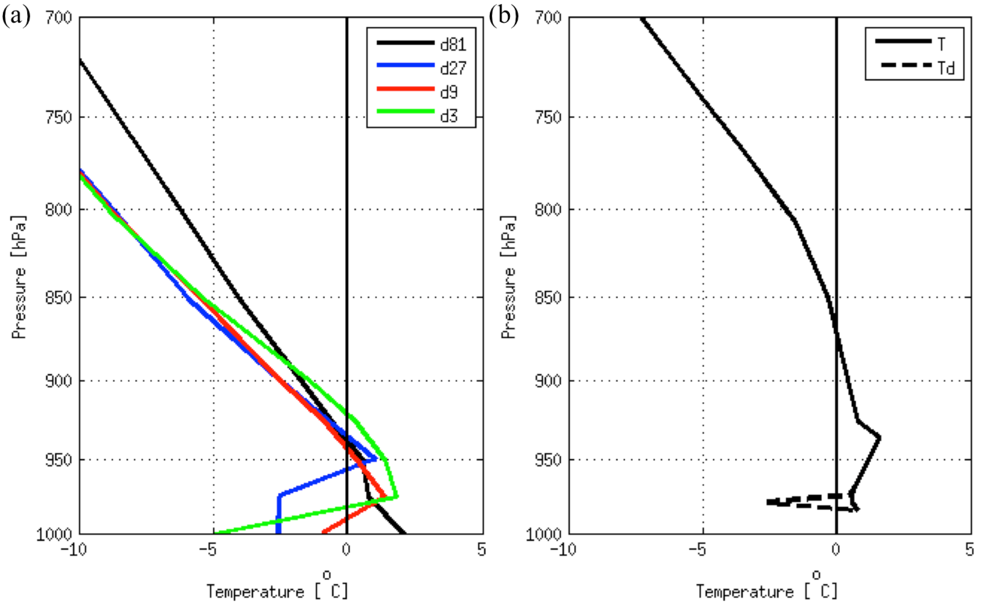
• The vertical temperature structure is also impacted by the model horizontal resolution. For example, a simulation with a mesh of 81 km would lead to rain at the surface, whereas the 3‑km one would be associated with freezing rain. For instance, no refreezing layer and temperature inversion are found at lower levels for the simulation with grid spacing of 81 km. Furthermore, the depth and temperature of the melting layer varies significantly across model resolutions, which is directly linked to the type of precipitation.
• A pragmatic theoretical cost argument has been developed, suggesting a climatological framework to use the cascade method for studying specific high-impact weather of interest using very high-resolution regional climate modeling.

In conclusion, considering that the wind direction in the SLRV is closely related to high-impact weather events, such as freezing rain (e.g., [31]), this constitutes a major potential added value of high-resolution simulations. The results confirmed the importance of getting the accurate wind speed and direction to solve for the type of precipitation when the temperature is near 0 °C. It appears that 3-km grid spacing is the best suited to obtain the appropriate temperature inversion and the good representation of SLRV wind channelling. This study lends confidence to the idea that climate simulations and projections at the kilometer scale could soon become operationally feasible, thus offering interesting perspectives for resolving features that are out of reach with coarser-mesh models.

Several challenges remain for the operational implementation of the proposed cascade strategy, including the adjustment of the subgrid-scale physical parameterizations as a function of the model’s grid mesh remaining a distinct challenge. In particular, for deep convection across the “grey zone”, there is currently little consensus in the research community as to the exact mesh size where the use of the moist convection parameterization becomes necessary. This issue needs to be addressed adequately before the simulation of convective precipitation systems for climate application can fully benefit from the cascade approach down to kilometer-scale meshes.

References

1. Parry, M.L.; Canziani, O.F.; Palutikof, J.P.; van der Linden, P.J.; Hanson, C.E. IPCC: Climate Change 2007: Impacts, Adaptation and Vulnerability; Cambridge University Press: Cambridge, UK, 2007; p. 976. [Google Scholar]
2. IPCC. Climate Change 2013: The Physical Science Basis; Stocker, T.F., Qin, D., Plattner, G.K., Tignor, M., Allen, S.K., Boschung, J., Nauels, A., Xia, Y., Bex, V., Midgley, P.M., Eds.; Cambridge University Press: Cambridge, UK, 2013; p. 1535. [Google Scholar]
3. Mearns, L.O.; Schneider, S.H.; Thompson, S.L.; McDaniel, L.R. Analysis of climate variability in General Circulation Models: Comparison with observations and changes in variability in 2×CO2 experiments. J. Geophys. Res. 1990, 95, 20469–20520. [Google Scholar] [CrossRef]
4. Christensen, J.H.; Hewitson, B.; Busuioc, A.; Chen, A.; Gao, X.; Held, I.; Jones, R.; Kolli, R.K.; Kwon, W.-T.; Laprise, R.; et al. Regional climate projections. In Climate Change 2007: The Physical Science Basis; Contribution of Working Group I (WGI) to the Fourth Assessment Report (AR4) of the Intergovernmental Panel on Climate Change (IPCC); Solomon, S., Qin, D., Manning, M., Chen, X., Marquis, M., Averyt, K.B., Tignor, M., Miller, H.L., Eds.; Cambridge University Press: Cambridge, UK; New York, NY, USA, 2007; pp. 918–925. [Google Scholar]
5. Giorgi, F.; Coppola, E. Does the model regional bias affect the projected regional climate change? An analysis of global model projections. Clim. Chang. 2010, 100, 787–795. [Google Scholar] [CrossRef]
6. Dickinson, R.E.; Errico, R.M.; Giorgi, F.; Bates, G.T. A regional climate model for the western United States. Clim. Chang. 1989, 15, 383–422. [Google Scholar]
7. Giorgi, F. Simulation of regional climate using a limited area model nested in a general circulation model. J. Clim. 1990, 3, 941–963. [Google Scholar] [CrossRef]
8. Von Storch, H.; Langenberg, H.; Feser, F. A spectral nudging technique for dynamical downscaling purposes. Mon. Weather Rev. 2000, 128, 3664–3673. [Google Scholar] [CrossRef]
9. Nikulin, G.; Jones, C.; Giorgi, F.; Asrar, G.; Büchner, M.; Cerezo-Mota, R.; Christensen, O.B.; Déqué, M.; Fernandez, J.; Hänsler, A.; et al. Precipitation climatology in an ensemble of CORDEX-Africa regional climate simulations. J. Clim. 2012, 25, 6057–6078. [Google Scholar] [CrossRef]
10. Giorgi, F. Future directions for CORDEX: Emerging issues concerning Regional climate projections. In Proceedings of the ICRC 2013, Brussels, Belgium, 4–7 November 2013.
11. Hong, S.-Y.; Kanamitsu, M. Dynamical downscaling: Fundamental issue from an NWP point of view and recommendations. Asia-Pac. J. Atmos. Sci. 2014, 50, 83–104. [Google Scholar] [CrossRef]
12. Kendon, E.J.; Roberts, N.M.; Senior, C.A.; Roberts, M.J. Realism of rainfall in a very high-resolution regional climate model. J. Clim. 2012, 25, 5791–5806. [Google Scholar] [CrossRef]
13. Ban, N.; Schmidli, J.; Schär, C. Evaluation of the convection-resolving regional climate modeling approach in decade-long simulations. J. Geophys. Res. Atmos. 2014, 119, 7889–7907. [Google Scholar] [CrossRef]
14. Jacob, D.; Petersen, J.; Eggert, B.; Alias, A.; Christensen, O.B.; Bouwer, L.M.; Braun, A.; Colette, A.; Déqué, M.; Georgievski, G.; et al. EURO-CORDEX: New high-reolution climate change projections for European impact research. Reg. Environ. Chang. 2014, 14, 563–578. [Google Scholar] [CrossRef]
15. Lucas-Picher, P.; Riboust, P.; Somot, S.; Laprise, R. Reconstruction of the spring 2011 Richelieu River flood by two regional climate models and a hydrological model. J. Hydrometeor. 2014. [Google Scholar] [CrossRef]
16. Hart, K.A.; Steenburgh, W.J.; Onton, D.J. Model forecast improvements with decreased horizontal grid spacing over finescale intermountain orography during the 2002 Olympic Winter Games. Weather Forecast. 2005, 20, 558–576. [Google Scholar] [CrossRef]
17. Lean, H.W.; Clark, P.A.; Dixon, M.; Roberts, N.M.; Fitch, A.; Forbes, R.; Halliwell, C. Characteristics of high-resolution versions of the Met Office Unified Model for forecasting convection over the United Kingdom. Mon. Weather Rev. 2008, 136, 3408–3424. [Google Scholar] [CrossRef]
18. Mailhot, J.; Milbrandt, J.A.; Giguère, A.; McTaggart-Cowan, R.; Erfani, A.; Denis, B.; Glazer, A.; Vallée, M. An experimental high resolution forecast system during the Vancouver 2010 winter Olympic and Paralympic games. Pure Appl. Geophys. 2014, 171, 209–229. [Google Scholar] [CrossRef]
19. Coen, J.; Cameron, M.; Michalakes, J.; Patton, E.; Riggan, P.; Yedinak, K. WRF-fire: Coupled weather-wildland fire modeling with the weather research and forecasting model. J. Appl. Meteor. Climatol. 2013, 52, 16–38. [Google Scholar] [CrossRef]
20. Trapp, R.J.; Halvorson, B.A.; Diffenbaugh, N.S. Telescoping, multimodel approaches to evaluate extreme convective weather under future climates. J. Geophys. Res. 2007, 112, 1–13. [Google Scholar]
21. Prein, A.F.; Truhetz, H.; Suklistch, M.; Gobiet, A. Evaluation of the Local Climate Model Intercomparison Project (LocMIP) simulations. WegCenter Rep. 2011, 41, 27–57. [Google Scholar]
22. Stiperski, I.; Ivančan-Picek, B.; Grubišić, V.; Bajić, A. Complex bora flow in the lee of southern velebit. Quart. J. R. Meteorol. Soc. 2012, 138, 1490–1506. [Google Scholar] [CrossRef]
23. Mahoney, K.; Alexander, M.; Scott, J.D.; Barsugli, J. High-resolution downscaled simulations of warm-season extreme precipitation events in the Colorado Front Range under past and future climates. J. Clim. 2013, 26, 8671–8689. [Google Scholar] [CrossRef]
24. Wang, C.; Jones, R.; Perry, M.; Johnson, C.; Clark, P. Using ultrahigh-resolution regional climate model to predict local climatology. Quart. J. R. Meteorol. Soc. 2013. [Google Scholar] [CrossRef]
25. Yeung, J.K.; Smith, J.A.; Villarini, G.; Ntelekos, A.A.; Baeck, M.L.; Krajewski, W.F. Analyses of the warm season rainfall climatology of the northeastern US using regional climate model simulations and radar rainfall fields. Adv. Water Resour. 2011, 34, 184–204. [Google Scholar] [CrossRef]
26. BALTEX: The Baltic Sea Experiment: 3rd Lund Regional-scale Climate Modelling Workshop, 21st Century Challenges in Regional Climate Modelling. Lund, Sweden, 16–19 June 2014; Available online: http://www.baltex-research.eu/RCM2014/ (accessed on 19 December 2014).
27. Leduc, M.; Laprise, R. Regional Climate Model sensitivity to domain size. Clim. Dyn. 2009, 32, 833–854. [Google Scholar] [CrossRef]
28. Hill, G.E. Grid telescoping in numerical weather prediction. J. Appl. Meteor. 1968, 7, 29–38. [Google Scholar] [CrossRef]
29. Chen, J.H.; Miyakoda, K. A nested grid computation for the barotropic free surface atmosphere. Mon. Weather Rev. 1974, 102, 181–190. [Google Scholar] [CrossRef]
30. Rife, D.L.; Davis, C.A.; Knievel, J.C. Temporal changes in wind as objects for evaluating mesoscale numerical weather prediction. Weather Forecast. 2009, 24, 1374–1389. [Google Scholar] [CrossRef]
31. Roebber, P.J.; Gyakum, J.R. Orographic influences on the mesoscale structure of the 1998 ice storm. Mon. Weather Rev. 2003, 131, 27–50. [Google Scholar] [CrossRef]
32. Hernández-Díaz, L.; Laprise, R.; Sushama, L.; Martynov, A.; Winger, K.; Dugas, B. Climate simulation over CORDEX Africa domain using the fifth-generation Canadian Regional Climate Model (CRCM5). Clim. Dyn. 2013, 40, 1415–1433. [Google Scholar] [CrossRef]
33. Martynov, A.; Laprise, R.; Sushama, L.; Winger, K.; Šeparović, L.; Dugas, B. Reanalysis-driven climate simulation over CORDEX North America domain using the Canadian Regional Climate Model, version 5: Model performance evaluation. Clim. Dyn. 2013, 41, 2973–3005. [Google Scholar] [CrossRef] [Green Version]
34. Šeparović, L.; Alexandru, A.; Laprise, R.; Martynov, A.; Sushama, L.; Winger, K.; Tete, K.; Valin, M. Present climate and climate change over North America as simulated by the fifth-generation Canadian Regional Climate Model (CRCM5). Clim. Dyn. 2013, 41, 3167–3201. [Google Scholar]
35. Côté, J.; Gravel, S.; Méthot, A.; Patoine, A.; Roch, M.; Staniforth, A. The operational CMC-MRB Global Environmental Multiscale (GEM) model: Part I—Design considerations and formulation. Mon. Weather Rev. 1998, 126, 1373–1395. [Google Scholar] [CrossRef]
36. Côté, J.; Desmarais, J.-G.; Gravel, S.; Méthot, A.; Patoine, A.; Roch, M.; Staniforth, A. The operational CMC-MRB Global Environmental Multiscale (GEM) model: Part II–Results. Mon. Weather Rev. 1998, 126, 1397–1418. [Google Scholar] [CrossRef]
37. Yeh, K.S.; Gravel, S.; Méthot, A.; Patoine, A.; Roch, M.; Staniforth, A. The CMC-MRB global environmental multiscale (GEM) model. Part III: Non-hydrostatic formulation. Mon. Weather Rev. 2002, 130, 339–356. [Google Scholar] [CrossRef]
38. Laprise, R. The Euler equation of motion with hydrostatic pressure as independent coordinate. Mon. Weather Rev. 1992, 120, 197–207. [Google Scholar] [CrossRef]
39. Davies, H.C. A lateral boundary formulation for multi-level prediction models. Quart. J. R. Meteorol. Soc. 1976, 102, 405–418. [Google Scholar]
40. Verseghy, D.L. The Canadian land surface scheme (CLASS): Its history and future. Atm.-Ocean 2000, 38, 1–13. [Google Scholar] [CrossRef]
41. Verseghy, D.L. The Canadian Land Surface Scheme: Technical Documentation, Version 3.4; Climate Research Division, Science and Technology Branch, Environment Canada: Dorval, QC, Canada, 2008. [Google Scholar]
42. Li, J.; Barker, H.W. A radiation algorithm with correlated-k distribution. Part-I: Local thermal equilibrium. J. Atmos. Sci. 2005, 62, 286–309. [Google Scholar] [CrossRef]
43. Benoit, R.; Côté, J.; Mailhot, J. Inclusion of TKE boundary layer parameterization in the Canadian Regional Finite-Element Model. Mon. Weather Rev. 1989, 117, 1726–1750. [Google Scholar] [CrossRef]
44. Delage, Y.; Girard, C. Stability functions correct at the free convection limit and consistent for both the surface and Ekman layers. Bound. Layer Meteor. 1992, 58, 19–31. [Google Scholar] [CrossRef]
45. Delage, Y. Parameterising sub-grid scale vertical transport in atmospheric models under statically stable conditions. Bound. Layer Meteor. 1997, 82, 23–48. [Google Scholar] [CrossRef]
46. Tiedtke, M. A comprehensive mass flux scheme for cumulus parameterization in large-scale models. Mon. Weather Rev. 1989, 117, 1779–1800. [Google Scholar] [CrossRef]
47. Kuo, H.L. On formation and intensification of tropical cyclones through latent heat release by cumulus convection. J. Atmos. Sci. 1965, 22, 40–63. [Google Scholar] [CrossRef]
48. Bélair, S.; Mailhot, J.; Girard, C.; Vaillancourt, P. Boundary-layer and shallow cumulus clouds in a medium-range forecast of a large-scale weather system. Mon. Weather Rev. 2005, 133, 1938–1960. [Google Scholar] [CrossRef]
49. Molinari, J.; Dudek, M. Parameterization of convective precipitation in mesoscale numerical models: A critical review. Mon. Weather Rev. 1992, 120, 326–344. [Google Scholar] [CrossRef]
50. Arakawa, A. The cumulus parameterization problem: Past, present and future. J. Clim. 2004, 17, 2493–2525. [Google Scholar] [CrossRef]
51. Piriou, J.M.; Redelsperger, J.-L.; Geleyn, J.-F.; Lafore, J.-P.; Guichard, F. An approach for convective parameterization with memory: Separating microphysics and transport in grid-scale equations. J. Atmos. Sci. 2007, 64, 4127–4139. [Google Scholar] [CrossRef]
52. Gérard, L. An integrated package for subgrid convection, clouds and precipitation compatible with meso-gamma scales. Quart. J. R. Meteorol. Soc. 2007, 133, 711–730. [Google Scholar] [CrossRef]
53. Gérard, L.; Piriou, J.M.; Brožková, R.; Geleyn, J.-F.; Banciu, D. Cloud and precipitation parameterization in a meso-gamma-scale operational weather prediction model. Mon. Weather Rev. 2009, 137, 3960–3977. [Google Scholar] [CrossRef]
54. Bengtsson, L.; Steinheimer, M.; Bechtold, P.; Geleyn, J.-F. A stochastic parametrization for deep convection using cellular automata. Quart. J. R. Meteorol. Soc. 2013, 139, 1533–1543. [Google Scholar] [CrossRef]
55. Sundqvist, H.; Berge, E.; Kristjansson, J.E. Condensation and cloud parameterization studies with a mesoscale numerical weather prediction model. Mon. Weather Rev. 1989, 117, 1641–1657. [Google Scholar] [CrossRef]
56. Bourgouin, P. A method to determine precipitation types. Weather Forecast. 2000, 15, 583–592. [Google Scholar] [CrossRef]
57. Kain, J.S.; Fritsch, J.M. A one-dimensional entraining/detraining plume model and application in convective parameterization. J. Atmos. Sci. 1990, 47, 2784–2802. [Google Scholar] [CrossRef]
58. McFarlane, N.A. The effect of orographically excited gravity-wave drag on the circulation of the lower stratosphere and troposphere. J. Atmos. Sci. 1987, 44, 1175–1800. [Google Scholar]
59. Zadra, A.; Roch, M.; Laroche, S.; Charron, M. The subgrid-scale orographic blocking parametrization of the GEM Model. Atm.-Ocean 2003, 41, 155–170. [Google Scholar] [CrossRef]
60. Milbrandt, J.A.; Yau, M.K. A multimoment bulk microphysics parameterization. Part I: Analysis of the role of the spectral shape parameter. J. Atmos. Sci. 2005, 62, 3051–3064. [Google Scholar] [CrossRef]
61. Milbrandt, J.A.; Yau, M.K. A multimoment bulk microphysics parameterization. Part II: A proposed three-moment closure and scheme description. J. Atmos. Sci. 2005, 62, 3065–3081. [Google Scholar] [CrossRef]
62. Simmons, A.; Uppala, S.; Dee, D.; Kobayashi, S. ERA-Interim: New ECMWF reanalysis products from 1989 onwards. ECMWF Newslett. 2007, 110, 26–35. [Google Scholar]
63. Boer, G.J. Predictability regimes in atmospheric flow. Mon. Weather Rev. 1994, 122, 2285–2295. [Google Scholar] [CrossRef]
64. Lilly, D.K.; Bassett, G.; Droegemeier, K.; Bartello, P. Stratified turbulence in the atmospheric mesoscales. Theoret. Comput. Fluid Dyn. 1998, 11, 139–153. [Google Scholar] [CrossRef]
65. Pielke, R.A. A recommended specific definition of “resolution”. Agric. For. Meteorol. 1991, 55, 345–349. [Google Scholar] [CrossRef]
66. De Elía, R.; Laprise, R.; Denis, B. Forecasting skill limits of nested, limited-area models: A perfect-model approach. Mon. Weather Rev. 2002, 130, 2006–2023. [Google Scholar] [CrossRef]
67. Charney, J.G. Geostrophic turbulence. J. Atmos. Sci. 1971, 28, 1087–1095. [Google Scholar] [CrossRef]
68. Boer, G.J.; Shepherd, T.G. Large-scale two-dimensional turbulence in the atmosphere. J. Atmos. Sci. 1983, 40, 164–184. [Google Scholar]
69. Nastrom, G.D.; Gage, K.S. A climatology of atmospheric wavenumber spectra of wind and temperature observed by commercial aircraft. J. Atmos. Sci. 1985, 42, 950–960. [Google Scholar] [CrossRef]
70. Gage, K.S.; Nastrom, G.D. Theoretical interpretation of atmospheric wavenumber spectra of wind and temperature observed by commercial aircraft during GASP. J. Atmos. Sci. 1986, 43, 729–740. [Google Scholar] [CrossRef]
71. Denis, B.; Côté, J.; Laprise, R. Spectral decomposition of two-dimensional atmospheric fields on limited-area domains using the Discrete Cosine Transform (DCT). Mon. Weather Rev. 2002, 130, 1812–1829. [Google Scholar] [CrossRef]
72. Skamarock, W.C. Evaluating mesoscale NWP models using kinetic energy spectra. Mon. Weather Rev. 2004, 132, 3019–3032. [Google Scholar] [CrossRef]
73. Durran, D.R. Numerical Methods for Fluid Dynamics: With Applications to Geophysics; Springer: New York, NY, USA, 2010; Volume 32, p. 516. [Google Scholar]
74. Leith, C.E. Diffusion approximation for two-dimensional turbulence. Phys. Fluids 1968, 11, 671–673. [Google Scholar] [CrossRef]
75. Koshyk, J.N.; Hamilton, K. The horizontal kinetic energy spectrum and spectral budget simulated by high-resolution troposphere-stratosphere-mesosphere GCM. J. Atmos. Sci. 2001, 58, 329–348. [Google Scholar] [CrossRef]
76. Historical Climate Data. Available online: http://climate.weather.gc.ca/advanceSearch/searchHistoricData_e.html/ (accessed on 25 March 2015).
77. Cholette, M. Méthode de Télescopage Appliquée au MRCC5 Pour une Étude de Faisabilité d’un Modèle Régional de Climat de Très Haute Résolution. M.Sc. Dissertation, Department Earth and Atmospheric Sciences, Université du Québec à Montréal, Montréal, QC, Canada, 2013; p. 101. [Google Scholar]
78. Carrera, M.L.; Gyakum, J.R.; Lin, C.A. Observational study of wind channeling within the St-Lawrence River valley. J. Appl. Meteor. Climatol. 2009, 48, 2341–2361. [Google Scholar] [CrossRef]
79. MétéoCentre: Centre Météo UQAM Montréal | La météo en temps réel pour le Québec, le Canada, les États-Unis et l’Europe. Available online: http://meteocentre.com/ (accessed on 26 March 2015).
80. Thériault, J.M.; Stewart, R. A parameterization of the microphysical processes forming many types of winter precipitation. J. Atmos. Sci. 2010, 67, 1492–1508. [Google Scholar] [CrossRef]
81. University of Wyoming, College of Engineering, Department of Atmospheric Science. Available online: http://weather.uwyo.edu/wyoming/ (accessed on 25 March 2015).
82. Lindzen, R.S.; Fox-Rabinowitz, M. Consistent vertical and horizontal resolution. Mon. Weather Rev. 1989, 117, 2575–2583. [Google Scholar] [CrossRef]
83. Robert, A. A stable numerical integration scheme for the primitive meteorological equations. Atm.-Ocean 1981, 19, 35–46. [Google Scholar] [CrossRef]
84. Clark, T.L.; Farley, R.D. Severe downslope windstorm calculations in two and three spatial dimensions using anelastic interactive grid nesting: A possible mechanism for gustiness. J. Atmos. Sci. 1984, 41, 329–350. [Google Scholar] [CrossRef]
85. Beck, A.; Ahrens, B.; Stadlbacher, K. Impact of nesting strategies in dynamical downscaling of reanalysis data. Geophys. Res. Lett. 2004. [Google Scholar] [CrossRef]
86. Suklitsch, M.; Gobiet, A.; Leuprecht, A.; Frei, C. High resolution sensitivity studies with the regional climate model CCLM in the Alpine Region. Meteorol. Z. 2008, 17, 467–476. [Google Scholar] [CrossRef]
87. Denis, B.; Laprise, R.; Caya, D. Sensitivity of a regional climate model to the resolution of the lateral boundary conditions. Clim. Dyn. 2003, 20, 107–126. [Google Scholar]
88. Razy, A.; Milrad, S.M.; Atallah, E.H.; Gyakum, J.R. Synoptic-scale environments conductive to orographic impacts on cold-season surface wind regimes at Montreal, Quebec. J. Appl. Meteor. Climatol. 2012, 51, 598–616. [Google Scholar] [CrossRef]