3.1. Control Simulation (CNTRL)
The CNTRL simulations comprised of ten-member ensembles. The simulations were driven by the NOAA Optimum Interpolation (OI) SST V2 long-term climatological mean prescribed over the entire domain (
Figure 2). The initial and lateral boundary conditions were four times daily NCEP Reanalysis climatologies for 1971–2000. Each ensemble member was created by randomly modifying the specific humidity at each grid cell in the lateral boundaries through the simulation period. The amplitude of the perturbation is only one-tenth of one percent of the original specific humidity values, and hence the random relative humidity modification only minutely perturbs the initial and lateral boundary conditions, without measurable effects on the primary forcing. The 10-member ensemble mean rainfall rate for CNTRL was used as a reference to assess changes in simulated rainfall rates associated with SST forcing over different ocean basins.
The CNTRL ensemble mean rainfall rate produced a realistic June–September rainfall distribution over Western Ethiopia (
Figure 3a) that compared well with observed rainfall climatology for 1970–1999 (
Figure 3b). However, there are significant differences between observed and simulated rainfall rates over Northwestern and Eastern Ethiopia, with the simulations showing much drier rainfall rates in Eastern Ethiopia. Comparison of
Figure 3a,b with Section 5 of [
9] (June-September simulated-observed rainfall rates, bottom panel) shows that the large simulated rainfall rate (>10 mm·day
−1) in Northwest Ethiopia also was reproduced in the average of 18 individual summer season simulations, and thus reflects the model’s wet bias in the region. In contrast, the eastward extension of moderate rainfall rate (>4 mm·day
−1) into Eastern Ethiopia was correctly simulated in [
9] (
Figure 7), but the climatologically (1971–2000 average) forced simulation produced little rainfall there. This disparity is the direct result of the absence of year-to-year variability in the simulation forced by climatological atmospheric and SST initial and boundary conditions, and not a result of model inaccuracy. The rainfall distributions and amounts for the peak monsoon rainfall months (July-August) are similar to the June to September simulation counterparts (
Figure 3c,d). Because of the importance of the peak rainy season months for Ethiopian monsoon rainfall, subsequent SST sensitivity comparisons will largely be limited to the July–August period.
Figure 3.
Comparison of CNTRL-simulated ensemble mean (left) and observed (right) rainfall rates (mm·day−1). (a) Simulated ensemble mean and (b) observed rainfall rates for June–September. (c) same as (a) but for July–August. (d) Same as (b) but for July–August. CNTRL is 10-member ensemble average obtained by specifying monthly varying 1971–2000 SST climatology with initial and boundary conditions obtained from 6-hourly and daily varying NCEP-NCAR Reanalysis climatology for 1971–2000.
The large-scale flow and temperature patterns for the CNTRL experiments are shown in
Figure 4 for July–August. There is a strong similarity between the observed mean seasonal flow (not shown) and the modeled flow forced by the climatological monthly SST and 6-hourly atmospheric fields. Major features of the simulated flow at 850 hPa for July–August (
Figure 4a) include warm surface temperatures in the equatorial trough zone, northerlies and northeasterlies from the Azores anticyclone, a well-established St. Helena anticyclone and associated southwesterlies in the Gulf of Guinea, westerlies across West Africa reaching Ethiopia, a zonally extended Mascarene anticyclone with strong Somali low level jet (LLJ), and southerly to southwesterly winds reaching Ethiopia. At 150 hPa (
Figure 4b), cooler (warmer) air dominates the equatorial tropics (subtropics), and the tropical easterly jet extends from India to Africa with wind speeds in excess of 20 m·s
−1 reaching Ethiopia. These circulation features are the major monsoon components affecting Ethiopian summer rainfall (e.g., [
10,
11]). The model-simulated large scale flow patterns largely are similar to the forcing reanalysis data, and will be used as a benchmark to assess the changes in large scale flow patterns associated with the SST sensitivity experiments.
Figure 4.
July–August wind (vector), resultant wind speed (dashed contour), and temperature (shading; K, color scale at right) patterns for CNTRL simulation for 850 hPa (top) and 150 hPa (bottom). Mean sea level pressure (hPa) is shown in top panel. Arrows give wind vectors (m·s−1, magnitude scale in lower right corner) and magnitude is also contoured (5 m·s−1 intervals). The border of Ethiopia is delineated by a solid bright red line.
3.2. Impacts of SST Variations in the Indian Ocean
The effects of SST variations in the Indian Ocean were examined by performing several sensitivity experiments (
Table 1). In the Northern Indian Ocean (NIO; 0°–25°N, 40°–75°E) and Southern Indian Ocean (SIO; 10°–40°S, 30°–80°E), SSTs were increased/decreased by 2K in the individual sectors while prescribing a 30-year average SST everywhere else in the model domain (
Figure 2). These experiments are denoted ±2K-NIO and ±2K-SIO, respectively. To examine the effects of zonally varying SSTs, westward linearly increasing/decreasing SST anomalies were added to the climatological SSTs over the Equatorial Indian Ocean while maintaining the 30-year average SSTs in the remaining model domain. In the first experiment (WwEcIO), the climatological SST over the Western Indian Ocean (10°S–10°N, 35°–70°E) was increased by a maximum of +2K off the coast of eastern Africa and then linearly decreased eastward to zero at 70°E. Over the Eastern Indian Ocean (10°S–10°N, 70°–100°E), the climatological SST was linearly further reduced eastwards with a maximum negative anomaly of −2K applied at the eastern extreme (100°E). This SST specification crudely follows a reversed SST gradient in the Indian Ocean associated with the Indian Ocean Dipole, as depicted in
Figure 2 of [
40]. In the second experiment for the Equatorial Indian Ocean (WcEwIO), the climatological SST over the Western Indian Ocean (10°S–10°N, 35°–70°E) was decreased by a maximum of −2K off the coast of Eastern Africa and then linearly increased eastward to zero at 70°E. Over the Eastern Indian Ocean (10°S–10°N, 70°–100°E), the climatological SST was linearly further increased eastwards with a maximum positive anomaly of +2K applied at the eastern extreme (100°E). All simulations (
Table 1) with the above-prescribed SST (±2K-NIO, ±2K-SIO, WwEcIO, and WcEwIO) were constrained by atmospheric initial and boundary conditions obtained from six-hourly and daily varying 1971–2000 NCEP Reanalysis climatologies.
For ease of comparison of the above six model simulations, the results are combined into composite figures that show the rainfall responses (
Figure 5), vertically integrated moisture fluxes (
Figure 6), and 850 hPa (
Figure 7) and 150 hPa (
Figure 8) large-scale circulation changes from CNTRL. This arrangement necessitates frequent cross-referencing between those figures when discussing rainfall responses and accompanying circulation changes associated with contrasting SST forcing couplets.
The simulation results show that, compared to CNTRL, warming of the NIO tends to create wetter conditions over much of the monsoon regions and drier weather over northwestern Ethiopia during July–August (
Figure 5a). The largest positive rainfall anomaly occurred in the central regions. In contrast, cooling of the NIO produced drier conditions in the Western and Central Ethiopia and wetter conditions in the northern regions (
Figure 5b). The rainfall responses to warmer and cooler SST anomaly forcing over the NIO were not identically opposite with each other, but had regional variations. For example, cooler SST forcing produced larger wet anomalies over Northern Ethiopia compared to the mildly drier conditions produced by a warmer anomaly-forcing counterpart.
The large scale atmospheric response to ±2K SST anomaly forcing over the NIO is summarized in
Figure 6a,b, which depict the vertically (1000–600 hPa) integrated zonal (left) and meridional (right) moisture fluxes at the western meridional (33°E, 3°–15°N) and southern zonal (3°N, 33°–48°E) Ethiopian boundaries, respectively. Comparison of the zonal and meridional moisture fluxes for CNTRL shows that the meridional moisture flux across the Ethiopian southern boundary generally is more than twice as large in magnitude as the zonal flux, and demonstrates that the southerlies are the primary moisture driver for Ethiopian June-September rainfall season. The +2K warming of the NIO increased the zonal moisture flux entering western Ethiopia, especially south of 9°N and north of 12°N compared to the simulation forced with climatological SST. For a -2K NIO SST anomaly forcing, the zonal moisture flux crossing the western boundary is reduced (enhanced) south (north) of 9°N compared to the climatological run. The nonsymmetrical moisture flux across the western boundary between the positive and negative anomaly forcing indicates the nonlinearity of the circulation response to the SST forcing. The meridional moisture flux across the Ethiopian southern boundary is higher for the +2K simulation than for the climatological run east of 37°E (
Figure 6b). Conversely, for the -2K NIO SST simulation the meridional moisture flux entering Southern Ethiopia at 3°N and between 33°–48°E is less than the moisture flux in the climatological SST simulation experiment.
Figure 5.
July-August simulated rainfall rate (mm·day
−1) ensemble differences from CNTRL for (
a) 2K sea surface temperature (SST) warming over the Northern Indian Ocean (NIO), (
b) 2K cooling over the NIO, (
c) linearly eastward decreasing SST over the Equatorial Indian Ocean (EIO), (
d) linearly eastward increasing SST over the EIO, (
e) 2K SST warming over the Southern Indian Ocean (SIO), and (
f) 2K SST cooling over the SIO. See
Figure 2 for ocean basin definition. See
Table 1 for description of experiments.
The increase in moisture flux for the +2K NIO SSTA forcing occurred in conjunction with large negative (positive) geopotential height (temperature) anomalies and deepening of the monsoon trough east of 40°E. Other notable synoptic features associated with the +2K NIO SSTA simulation include intensification of the Mascarene high and associated anomalous anticyclone in the southern Indian Ocean and strengthening of the LLJ at low levels (
Figure 7a). In the upper troposphere, anomalous anticyclonic circulation in the Eastern Mediterranean Sea tended to strengthen the tropical easterly jet (TEJ) east of 30°E (
Figure 8a). Although low-level cooler and upper-level warmer temperature anomalies appeared to increase atmospheric stability more in the +2K NIO simulation than in the CNTRL, the vertical structure of moist static stability still showed a conditionally unstable atmosphere in the +2K NIO experiment across much of Ethiopia. For the -2K NIO simulation, positive anomalous geopotential height in the monsoon trough, northerly anomalous flow over the Indian Ocean, negative anomalous geopotential height and anomalous cyclonic circulation in the Southern Indian Ocean weakened the monsoon system at lower levels (
Figure 7b). In the upper troposphere, westerly anomalous flow appeared to weaken the TEJ across Ethiopia (
Figure 8b), which can lead to a locally weaker monsoon rainfall (
Figure 5b).
Figure 6.
Vertically (1000–600 hPa) integrated zonal and meridional moisture fluxes averaged over July–August for warmer/cooler sea surface temperature (SST) anomaly forcing across the Indian Ocean. (
a) Zonal moisture fluxes for the Northern Indian Ocean warming/cooling experiments. (
b) Same as (a) except for meridional fluxes. (
c) Zonal moisture flux for the linearly eastward decreasing/increasing SST forcing experiments over the Equatorial Indian Ocean. (
d) Same as (c) except for meridional fluxes. (
e) Same as (a) except for the Southern Indian Ocean (SIO). (
f) Same as (b) except for the SIO. CNTRL is 10-member ensemble average obtained by specifying monthly varying 1971–2000 SST climatology with initial and boundary conditions obtained from 6-hourly and daily varying NCEP-NCAR Reanalysis climatology for 1971–2000. WwEcIO and WcEwIO are simulations with west-to-east linearly decreasing (increasing) ± 2K SST anomaly forcing. See
Table 1 for description of experiments.
For WwEcIO experiment, the rainfall response to Equatorial Indian Ocean SST forcing was relatively weak during the peak monsoon months of July and August (
Figure 5c), but became strong in September, affecting the equatorial regions of Ethiopia, Somalia, and Kenya, each of which has seasonal rainfall peaks in April and October. For simulations with a reversed SST gradient experiment (WcEWIO), drier conditions prevail over Western Ethiopia and wetter conditions dominate over northeastern regions (
Figure 5d). Inspection of monthly simulated rainfall patterns (not shown) indicated that compared to CNTRL the WwEcIO simulation produced much higher rainfall rates in the Southern and Southeastern Ethiopia during September, whereas the WcEwIO produced near normal rainfall pattern in the Southern regions and wetter (drier) conditions in Northeastern (Western) Ethiopia. The WwEcIO simulated rainfall pattern is consistent with the effect of warm Indian Ocean dipole and positive ENSO events on Equatorial East Africa. Climatologically, the east-west SST anomaly gradient maximizes in October/November (e.g., [
40]), at the peak of the second short rainy season in Ethiopia and Kenya.
Figure 7.
Circulation changes from CNTL at 850 hPa averaged for July-August corresponding to SST anomaly (SSTA) forcing over the (
a,
b) Northern Indian Ocean (NIO; 0°–25°N, 40°–75°E); (
c,
d) Equatorial Indian Ocean (EqIO; 10°S–10°N, 70°–100°E); and (
e,
f) Southern Indian Ocean (SIO; 10°–40°S, 30°–80°E). Each panel shows differences in horizontal winds (vectors; m·s
−1, magnitude scale in lower right corner), temperature (shading; K, color scale at right), and geopotential height (contours; gpm) between the perturbed SSTA forcing experiments and CNTRL. Differences of geopotential heights are contoured every 5 gpm. Anomaly vectors are plotted for resultant magnitudes of at least 1 m·s
−1 only. The border of Ethiopia is delineated in solid red line. See
Table 1 for description of experiments.
Figure 8.
Circulation changes from CNTL at 150 hPa averaged for July-August corresponding to SST anomaly (SSTA) forcing over the (
a,
b) Northern Indian Ocean (NIO; 0°–25°N, 40°–75°E); (
c,
d) Equatorial Indian Ocean (EqIO; 10°S–10°N, 70°–100°E); and (
e,
f) Southern Indian Ocean (SIO; 10°–40°S, 30°–80°E). Each panel shows differences in horizontal winds (vectors; m·s
−1, magnitude scale in lower right corner), temperature (shading; K, color scale at right), and geopotential height (contours; gpm) between the perturbed SSTA forcing experiments and CNTRL. Differences of geopotential heights are contoured every 50 gpm. Anomaly vectors are plotted for resultant magnitudes of at least 1 m·s
−1 only. The border of Ethiopia is delineated in solid red line. See
Table 1 for description of experiments.
The moisture fluxes associated with the Equatorial Indian Ocean simulations show reduced (marginally increased) zonal (meridional) fluxes for the WwEcIO, compared to CNTRL, across the entire latitudinal (longitudinal) cross sections (
Figure 6c,d). On the other hand, compared to CNTRL the WcEwIO simulation produced significantly larger zonal moisture fluxes, especially north of 9°N where much greater rainfall rate anomalies are observed. Although the overall amplitude of the meridional flux is higher than the zonal counterpart, there was a significant increase in zonal flux in Northern Ethiopia that compensated for the decrease in the meridional flux in the WcEwIO experiment.
The anomalous circulation signals associated with the Equatorial Indian Ocean SST gradient specification are much weaker than those found for the ±2K NIO simulations (
Figure 7,
Figure 8 middle panels). The major circulation anomalies for WwEcIO simulation are associated with the anomalous cyclonic circulation over the Arabian Sea and anomalous anticyclonic circulation over Northern Africa extending to the Red Sea at 850 hPa (
Figure 7c). Although there are weak southerly anomalies, the zonal wind anomalies are easterlies west of Ethiopia, consistent with the reduced zonal flux for WwEcIO in
Figure 6c. The WwEcIO SST forcing appeared to have a negligible effect on the strength of the Mascarene anticyclone. In the upper level (
Figure 8c), the zonal wind anomalies are weaker, indicating a lesser impact on the TEJ. However, the WcEwIO simulation produced stronger westerly anomalies reaching Northwest Ethiopia at 850 hPa and easterly (westerly) anomalies in Northern (Central) Ethiopia at 150 hPa that strengthen (weaken) the TEJ in Northern (Central and Western) Ethiopia (
Figure 7d and
Figure 8d).
The ±2K SIO SSTA forcing examines the effects of SST anomalies on the Mascarene high and its impact on Horn of Africa monsoonal rainfall. The warmer than CNTRL SIO SST anomaly forcing tended to increase simulated rainfall across much of the monsoon regions excluding the northern Rift Valley and extreme Northern Ethiopia, with larger wet anomalies being along the western lowlands and over Central and Eastern Ethiopia (
Figure 5e). In contrast, compared to CNTRL the -2K SIO SST anomaly forcing tended to produce drier conditions over Central Ethiopia (
Figure 5f). The asymmetry in the rainfall anomaly again is evident between the two contrasting SST forcing anomalies.
Compared to CNTRL, the increase (decrease) in zonal moisture flux associated with the +2K (-2K) SIO simulation is limited to south of 7°N, while there is no consistent difference in the meridional moisture fluxes between CNTRL and ±2K SIO simulations, with both anomaly simulations yielding lower meridional fluxes across all longitudes between 33°–48°E. In terms of large scale circulation changes, +2K SIO simulation reduced lower tropospheric pressure/geopotential height in the Western Indian Ocean and developed cyclonic circulation anomaly that wakened the Mascarene anticyclone (
Figure 7e). Associated with the development of the anomalous cyclonic flow, the meridional arm of the Intertropical Convergence Zone appeared to be strengthened along a region of warm temperature anomalies, but the monsoon southerlies are weakened. At 150 hPa, the westerly (easterly) anomalies in the Northern (Southern) Ethiopia indicate the weakening (strengthening) of the TEJ in those areas (
Figure 8e). The -2K SIO simulation produced the opposite circulation patterns, with anomalous southerlies (easterlies) at 850 (150) hPa, indicating the strengthening of the LLJ (
Figure 7f) and TEJ (
Figure 8f), respectively.
3.3. Rainfall Response to +1K, +2K, and +4K Atlantic and Indian Ocean SSTA Forcing
The effects of ocean-wide warming of the Atlantic and Indian Oceans on the Ethiopian monsoon rainfall were examined by adding +1K, +2K, and +4K SST anomalies to the monthly varying 1971–2000 climatological SSTs in the Atlantic (AT; 40°S–35°N, 30°W–15°E) and Indian Ocean (IO; 40°S–25°N, 30°–110°E) separately, while prescribing the climatological SSTs across the entire model domain, excluding the AT (or IO) in the respective AT (or IO) simulation (
Table 1). Initial and lateral boundary conditions are six-hourly and diurnally varying 30-year NCEP-NCAR Reanalysis climatologies for 1971–2000. These six experiments are denoted +1K-AT, +2K-AT, +4K-AT, +1K-IO, +2K-IO, and +4K-IO. Deviations in rainfall rates and large-scale circulation patterns were computed from CNTRL counterparts. For ease of comparison, the rainfall responses in the AT and IO simulations are displayed in a single figure. However, individual simulation results are discussed separately, beginning with the rainfall responses to AT warming and accompanying large scale circulation changes from CNTRL, followed by a discussion of the rainfall responses and associated circulation changes for counterpart IO simulations.
Figure 9.
Rainfall rate differences (mm·day
−1, color scale at right) from CNTRL averaged over July–August for simulations with (
a) +1K sea surface temperature anomaly (SSTA) forcing over the Atlantic Ocean (AT; 40°S–35°N, 30°W–15°E), (
b) 1K SSTA forcing over the Indian Ocean (IO; 40°S–25°N, 30°–110°E), (
c) +2K SSTA forcing over AT, (
d) +2K SSTA forcing over IO, (
e) +4K SSTA forcing over AT, and (
f) + 4K SSTA forcing over IO. Differences of ±5 mm·day
−1 rainfall rates are contoured. See
Table 1 for description of experiments.
Figure 9 shows rainfall rate deviations from CNTRL for July-August for the Atlantic and Indian Ocean SSTA forcing. Compared to CNTRL, mildly warmer (+1K) Atlantic Ocean SSTA forcing generally produces wetter conditions in Northern Ethiopia and drier conditions in the western and central regions (
Figure 9a). In particular, the drought prone regions of Northeastern Ethiopia appeared to benefit from the +1K Atlantic warming, with rainfall rates exceeding 5 mm·day
−1 occurring over the northern escarpments. On the other hand, the Blue Nile catchment is affected more severely with a much reduced rainfall rate of >10 mm·day
−1 in the +1K-AT simulation compared to CNTRL. For +2K-AT SSTA simulation (
Figure 9b), the wet anomaly over the northeastern regions disappeared while positive rainfall rate anomalies develop over Northwestern Ethiopia. At the same time, the large negative rainfall anomalies over the western and central regions became localized and less severe. Additionally, a weak positive rainfall anomaly developed in the southern Rift Valley regions. For the +4K-AT SSTA simulation (
Figure 9c), there was a general increase in simulated rainfall rate in the south and decrease in the northern Ethiopia plateau east of Lake Tana (refer to
Figure 1 for location of Lake Tana). The rainfall changes associated with the non-perturbed +1K, +2K, and +4K-AT warming simulations relative to a non-perturbed CNTRL simulation differed noticeably from the perturbed counterparts, and showed that warmer SSTA generally produce drier conditions over Western Ethiopia. The magnitude of the negative rainfall anomalies also increased as the forcing anomaly increased from +1K to +4K. Differences between the ensemble and non-perturbed simulations can be reduced significantly by increasing the perturbation ensemble size from 10 to 25–30.
The low-level (850 hPa) circulation changes associated with +1K, +2K, and +4K SSTA forcing over the Atlantic are shown in
Figure 10. For mild warming of +1K SSTA in the Atlantic, negative geopotential height anomalies developed across much of Africa west of 40°E and large positive anomalies (relative to the CNTRL) prevailed to the east centered over the India subcontinent (
Figure 10a). This pressure/geopotential height anomaly configuration likely reflects the warmer (cooler) temperature anomalies over Central and Eastern Africa (India), and created a large anomalous anticyclonic circulation located over India, and anomalous cyclonic centers over North Sudan/Chad and the Southwestern Indian Ocean. These circulation anomalies weakened the moist westerlies reaching Ethiopia and the southerlies from the Southern Indian Ocean, thereby contributing to the large negative precipitation anomalies in the Blue Nile catchment. The anticyclonic circulation over the Indian subcontinent and the cyclonic anomalies over the central Sahel and in the Mozambique Channel and surrounding areas weakened appreciably for the +2K and +4K SSTA simulations (
Figure 10b,c).
Figure 11 shows the 150-hPa circulation changes associated with +1K, +2K, and +4K SSTA forcing over the Atlantic Ocean. Consistent with the large lower tropospheric response to the +1K-AT SSTA forcing, there is significant reduction of upper tropospheric easterlies in the Indian Ocean in response to warm temperature anomalies and increasing geopotential height centered over the Bay of Bengal and a concomitant anomalous cyclonic flow over the Middle East/Western Asia. The easterly anomalies weakened for the +2K-AT and +4K-AT SSTA simulations, which led to a strengthening of the TEJ and subsequently improvement of the simulated rainfall compared to CNTRL over the Blue Nile catchment.
The largest rainfall response to SSTA forcing occurred for the Indian Ocean experiments (
Figure 9d–f). For the +1K-IO SSTA forcing, a large swath of monsoonal areas excluding parts of Eastern and Northeastern Ethiopia received reduced rainfall rates. In particular, much of the Blue Nile catchment experienced drier conditions, with negative rainfall rate anomalies exceeding 5 mm·day
−1 occurring over large area south of Lake Tana. For the +2K-IO SSTA simulation, the negative rainfall anomaly in the Blue Nile catchment persisted, while large positive rainfall anomalies developed over the drought prone regions of Northeastern Ethiopia. The dry and wet dipole patterns over the Blue Nile catchment and Northeastern Ethiopia persisted for the +4K-IO SSTA simulation, with >10 mm·day
−1 positive anomalies occurring over Wello in the northeastern region and >5 mm·day
−1 negative anomalies continuing in the northern Blue Nile catchment. As was the case for the non-perturbed AT simulations, there are noticeable differences between the non-perturbed and ensemble-based rainfall responses for IO SSTA forcing, with the +4K IO and AT SSTA simulations yielding comparable negative rainfall anomalies in the Western Ethiopia for the non-perturbed counterparts.
Figure 10.
Circulation changes from CNTRL at 850 hPa averaged over July-August for SST anomaly (SSTA) forcing of (
a) +1K, (
b) +2K, and (
c) +4K over the Atlantic Ocean (AT; 40°S–35°N, 30°W–15°E). Each panel shows differences in horizontal winds (vectors; m·s
−1, magnitude scale in lower right corner), temperature (shading; K, color scale at right), and geopotential height (contours; gpm) between the perturbed SSTA forcing experiments and CNTRL. Differences of geopotential heights are contoured every 5 gpm. Anomaly vectors are plotted for resultant magnitudes of at least 1 m·s
−1 only. The border of Ethiopia is delineated in solid red line. See
Table 1 for description of experiments.
Figure 11.
Circulation changes from CNTRL at 150 hPa averaged over July-August for SST anomaly (SSTA) forcing of (
a) +1K, (
b) +2K, and (
c) +4K over the Atlantic Ocean (AT; 40°S–35°N, 30°W–15°E). Each panel shows differences in horizontal winds (vectors; m·s
−1, magnitude scale in lower right corner), temperature (shading; K, color scale at right), and geopotential height (contours; gpm) between the perturbed SSTA forcing experiments and CNTRL. Differences of geopotential heights are contoured every 50 gpm. Anomaly vectors are plotted for resultant magnitudes of at least 1 m·s
−1 only. The border of Ethiopia is delineated in solid red line. See
Table 1 for description of experiments. See
Table 1 for description of experiments.
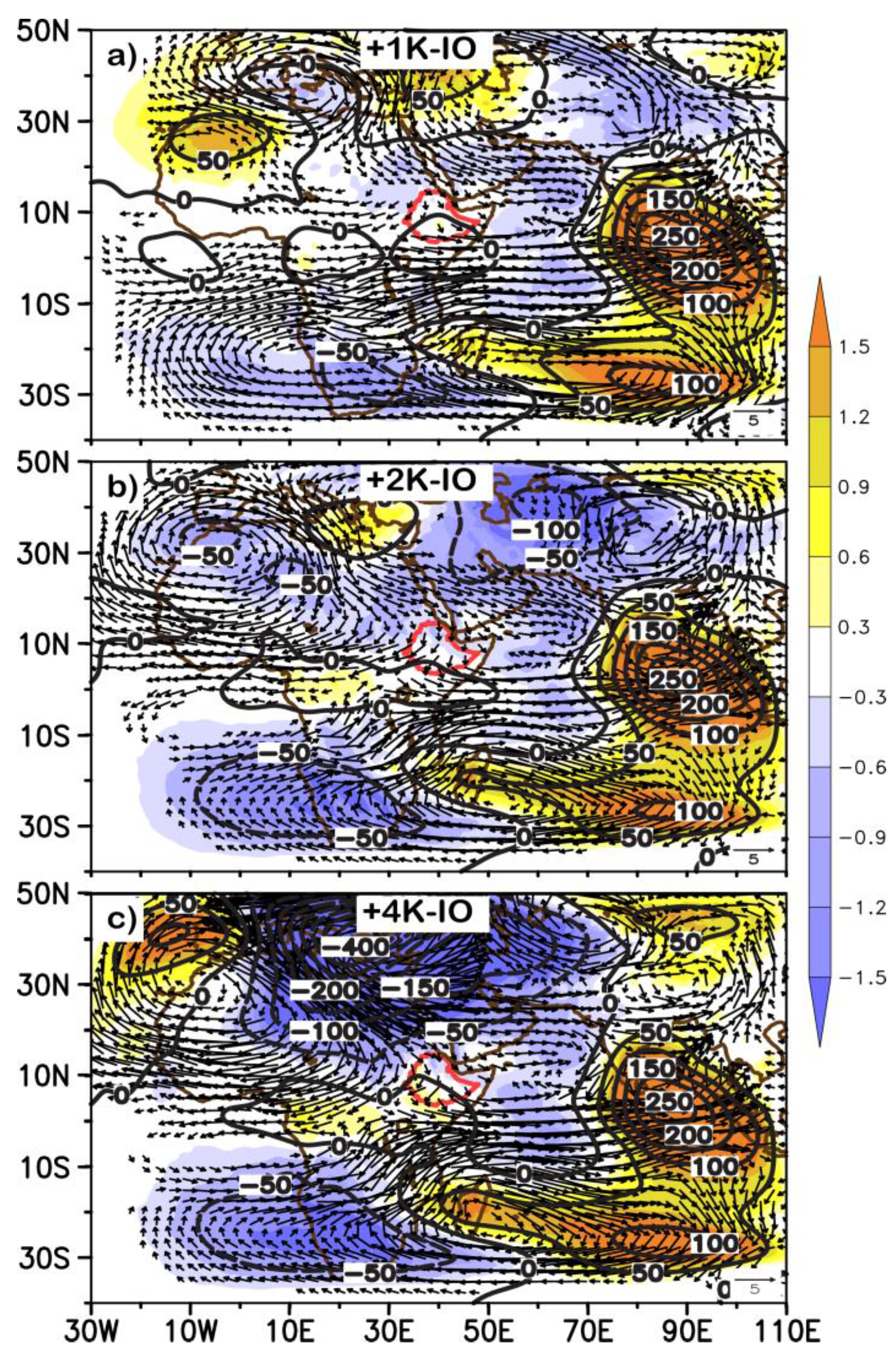
Figure 12 shows the circulation changes at 850 hPa associated with the Indian Ocean warming. For the +1K-IO SSTA, there is a slackening of the meridional pressure gradient associated with filling up of the heat lows over Africa and the monsoon trough over the Indian subcontinent. The easterly anomalies (anomalous cyclonic flow) over the Northern (Southern) Indian Ocean also weakened the LLJ (Mascarene anticyclone). While the weakening of the LLJ and Mascarene anticyclone continued for the +2K-IO and +4K-IO simulations, the meridional pressure gradient over the heat lows across Africa strengthened compared to CNTRL due to the weakened pressure/geopotential height fields in northern Africa. As a result, the increased westerly flow contributed to wet anomalies in Northern Ethiopia. The cooler temperature anomalies across the heat lows may not be consistent from the hydrothermal balance perspective (cooling leading to heavier air mass and higher pressure/geopotential height anomalies), but likely are due to evaporative cooling associated with the increased precipitation north of 12°N.
Figure 12.
Circulation changes from CNTRL at 850 hPa averaged over July-August for SST anomaly (SSTA) forcing of (
a) +1K, (
b) +2K, and (
c) +4K over the Indian Ocean (IO; 40°S–25°N, 30°–110°E). Each panel shows differences in horizontal winds (vectors; m·s
−1, magnitude scale in lower right corner), temperature (shading; K, color scale at right), and geopotential height (contours; gpm) between the perturbed SSTA forcing experiments and CNTRL. Differences of geopotential heights are contoured every 5 gpm. Anomaly vectors are plotted for resultant magnitudes of at least 1 m·s
−1 only. The border of Ethiopia is delineated in solid red line. See
Table 1 for description of experiments.
In the upper troposphere, there is a persistent warming and positive geopotential height anomaly response over the Eastern Indian Ocean and anticyclonic anomalous flow over Northwestern Africa associated with a basin-wide warming of the Indian Ocean (
Figure 13). The westerly anomalies in the Northern Indian Ocean (
Figure 13a) indicate the weakening of the TEJ, which likely contributed to the negative precipitation anomalies in the Blue Nile catchment. Of interest is the large incursion of cold air associated with the southward intrusion of midlatitude westerlies into Northeastern Africa in the +2K-IO and +4K-IO simulations (
Figure 13b,c). This upper level cold air incursion likely enhanced the instability and contributed to the positive precipitation anomalies in Northern Ethiopia.
Figure 13.
Circulation changes from CNTRL at 150 hPa averaged over July-August for SST anomaly (SSTA) forcing of (
a) +1K, (
b) +2K, and (
c) +4K over the Indian Ocean (IO; 40°S–25°N, 30°–110°E). Each panel shows differences in horizontal winds (vectors; m·s
−1, magnitude scale in lower right corner), temperature (shading; K, color scale at right), and geopotential height (contours; gpm) between the perturbed SSTA forcing experiments and CNTRL. Differences of geopotential heights are contoured every 50 gpm. Anomaly vectors are plotted for resultant magnitudes of at least 1 m·s
−1 only. The border of Ethiopia is delineated in solid red line. See
Table 1 for description of experiments. See
Table 1 for description of experiments.
The instability conditions associated with warmer Indian Ocean simulations is further examined from analysis of moist static energy (MSE), given by
MSE =
cpT +
Lq +
gz, where c
p is the specific heat of air at constant pressure, T is air temperature, L is the latent heat of vaporization, q is specific humidity, g is gravitational acceleration, and z is the geopotential height. Large MSE values at low levels destabilize the atmosphere, while a stable atmosphere exhibit increasing MSE with elevation (e.g., [
18,
19]).
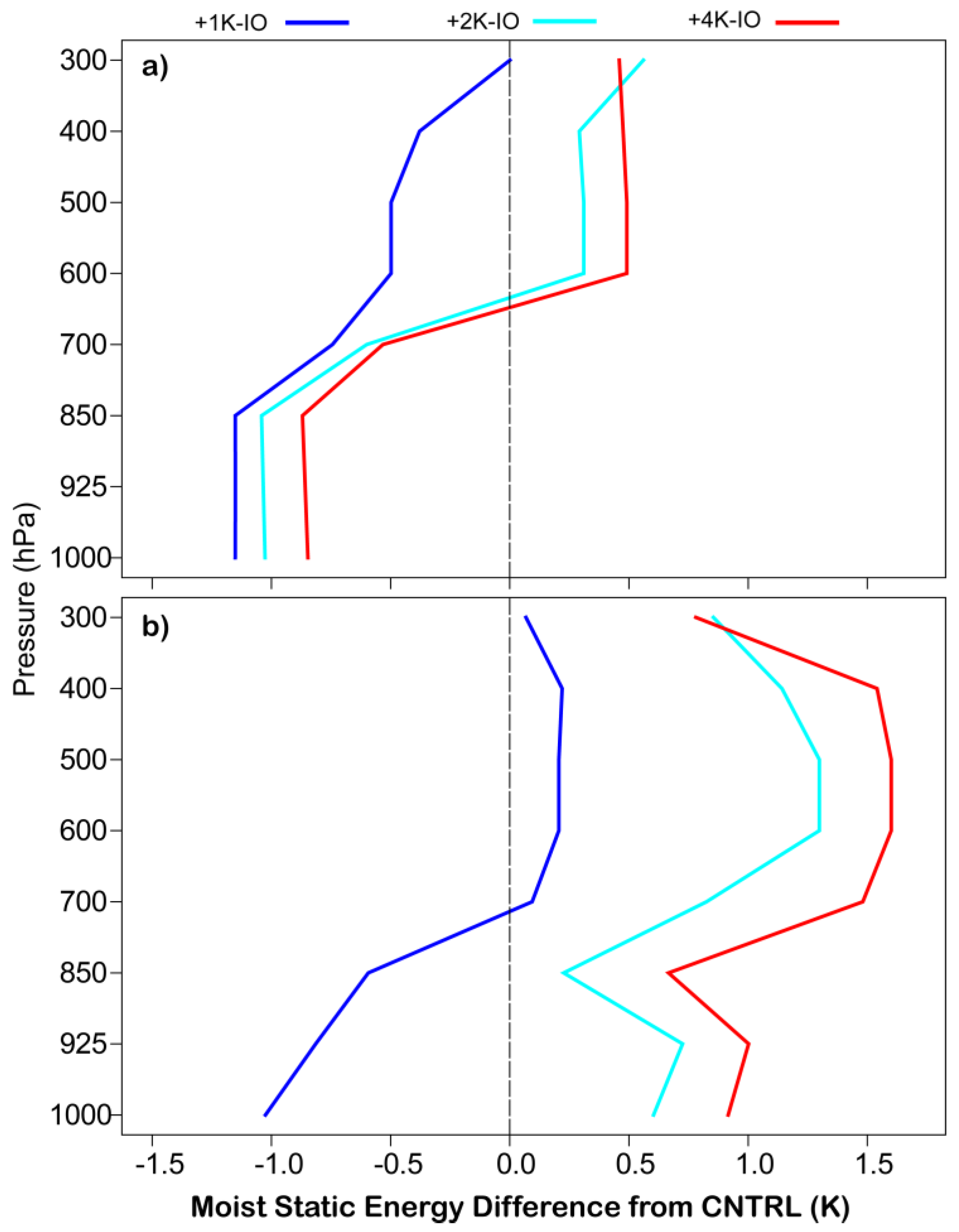
Figure 14 shows MSE deviations from CNTRL for the dry Blue Nile catchment and wet Northeastern Ethiopia for the +1K-IO, +2K-IO, and +4K-IO experiments. For the region with large negative precipitation anomalies, MSEs are lower than CNTRL at low levels, with no change up to 850 hPa compared to CNTRL, for which the MSE increases with height up to 850 hPa. The positive slope through 300 hPa indicates unfavorable conditions and more stably stratified atmosphere compared to CNTRL. For the wet northeastern region, the MSEs are higher than CNTRL with a shallower inversion layer extending to 925 hPa. The MSE steeply decreases up to 850 hPa for the +2K and +4K experiments for which large positive rainfall anomalies were simulated in Northeastern Ethiopia. Although the profiles for northeastern regions showed a weakening of the MSE gradient with height, the steep gradient further enhanced atmospheric instability and contributed to the positive precipitation anomalies in Northern Ethiopia.
Figure 14.
Vertical profiles of moist static energy (MSE) for warm Indian Ocean experiments. (
a) Deviations from CNTRL of moist static energy for the Blue Nile catchment (7°–11°N, 36°–40°E) for +1K (blue), +2K (cyan), and +4K (red) Indian Ocean simulations; (
b) Same as (a) except for MSE calculated for Northern Ethiopia (11°–14°N, 38°–40°E). MSE is given in units of K by normalizing it by the specific heat of air at constant pressure. See
Table 1 for description of experiments.


