Statistical Selection of the Optimum Models in the CMIP5 Dataset for Climate Change Projections of Indian Monsoon Rainfall

Abstract

Monsoons are the life and soul of India’s financial aspects, especially that of agribusiness in deciding cropping patterns. Around 80% of the yearly precipitation occurs from June to September amid monsoon season across India. Thus, its seasonal mean precipitation is crucial for agriculture and the national water supply. From the start of the 19th century, several studies have been conducted on the possible increments in Indian summer monsoon precipitation in the future. Unfortunately, none of them has endeavoured to discover the models whose yield give the best fit to the observed data. Here some statistical tests are performed to quantify the models of Coupled Model Inter-comparison Project 5 (CMIP5). Then, after, the Technique for Order Preference by Similarity to Ideal Solution (TOPSIS) method is used to select optimum models. It shows that four models, CCSM4, CESM1-CAM5, GFDL-CM3, and GFDL-ESM2G, best capture the pattern in Indian summer monsoon rainfall over the historical period (1871–2005). Further, Student’s t-test is utilized to estimate the significant changes in meteorological subdivisions of selected optimum models. Also, our results reveal the Indian meteorological subdivisions which are liable to encounter significant changes in mean at confidence levels that differ from 80% to 99%.

1. Introduction

Indeed, even post industrialization and fast development in the administration division, India transcendently remains a farming nation. Today, India ranks second all through the world in homestead yield from its farming and associated divisions. According to the information for the financial year 2011, agribusiness still keeps on contributing a noteworthy 16% to the national Gross Domestic Product (GDP) and 10% of the aggregate fare profit. Until now, around two-thirds of cultivated land specifically relied upon Indian summer monsoon rainfall. Accordingly, the variability of Indian summer monsoon rainfall assumes an essential part in the field of horticulture. Any anomaly in the seasonal rainfall influences the lives of a large number of individuals in the nation. Consequently, it is basic for government bodies to keep a nearby tab on the climate change patterns, particularly the changes in monsoon rainfall. This is more important in today’s scenario as the Intergovernmental Panel on Climate Change (IPCC) reports a significant change in the worldwide air temperatures amid the 21st century. This is going to have an immediate bearing on the season and intensity of rainfall the world over. Along these lines, suitable techniques are required to precisely anticipate these changing patterns and any climate conditions connected with it.

Future projections regarding global monsoon patterns are generally provided by means of Coupled Model Inter-comparison Project CMIP. As of late, the fifth appraisal report of the IPCC has introduced climate projections known as CMIP5 [1]. Under a worldwide temperature alteration, IPCC has anticipated that there can be a diverse change in the future All India Summer Monsoon Rainfall (AISMR) in its fifth assessment report [2]. These models have been produced taking into account the recently presented Representative Concentration Pathways (RCPs) for four distinct scenarios such as RCP 2.6, RCP 4.5, RCP 6.0, and RCP 8.5. In light of these four scenarios, the climate projections for the future can be assessed from various models accessible under the CMIP5 venture. It has been accounted that the models of the CMIP5 data set have a higher spatial resolution and henceforth are relied upon to yield significantly more accurate results [2]. Contrasting the past adaptation CMIP3 with new models of CMIP5, the simulated mean rainfall patterns over India are enhanced [3]. Then again, the model projections are more precise for parameters averaged over the entire globe. At the point when utilized for making projections at the regional level (national in particular), each of the models confronts certain constraints [4]. Diverse models lead to distinctive projections even under the same RCP scenarios. Henceforth, it becomes hard to assess a specific model to re-enact future precipitation forecasts. This is particularly valid if there should be an occurrence of local precipitation expectation in the Indian sub-continent. In that capacity, precipitation projection over India is still a matter of extraordinary exploration and investigative level headed discussion. A few models find almost no effect of warming on India’s monsoon rainfall [5,6,7,8], while a few models anticipate an increment in the all-India mean precipitation and Inter-Annual Variability (IAV) [9,10,11,12,13] for the compelling warming condition RCP 8.5. The ability of climate models in simulating the IAV is strongly related to their ability in re-enacting mean AISMR [13]. Most of the revised models in the CMIP5 dataset foresee a significant increase in Indian seasonal rainfall under the unchecked (business-as-usual) scenario [14]. From that point, the seasonal variation in precipitation over Asia-Pacific assumes a vital role in simulating the mean and, in addition, IAV of AISMR [15].

As of late, analytic studies have found that models predict clear future temperature increments but diverse changes in AISMR. Thus, to examine the variability of AISMR and the reliability of the projections, the data set of CMIP5 is isolated into different groups based on the nature of IAV. It has been reported that the group with the highest reliability projects a future reduction in light rainfall, and an increase in high to extreme rainfall [16]. Despite the fact that, in this study, the group of models used project increased IAV and, in addition, increased Indian rainfall, it is not reported which model predicts more accurately than others. It is additionally critical to dissect the progressions in AISMR in each of the meteorological subdivisions. For this reason, the first step is to choose the ideal CMIP5 models (for RCP 8.5) for precipitation projection in India, taking into account a statistical selection approach. Data for 20 CMIP5 models are compared with observations for the historical time period of 1871–2005. Six screening tests are used to assess the best fit in between the model and observed data for all-India rainfall. These include: (1) Z-value test, (2) correlation coefficient, (3) relative precipitation comparison (RPC) test, (4) probability function comparison (PDF) test, (5) root mean square error (RMSE) test, and (6) Student’s t-test. CMIP5 models are further hierarchically ranked using the Technique for Order Preference by Similarity to Ideal Solution (TOPSIS) technique. The projections of the chosen best model are then analyzed for the season of 2006–2100. The selected optimal models of this study agree with the results in a past study [16]. Thus, this may be considered as the results’ support and the quantitative outcomes of this study may be considered as a future reference.

2. Data and Methodology

This study uses information from 20 models that participated in CMIP5. Models are chosen in light of the accessibility of suitable data for comparison and projection purposes. Only those models for which historical data (1871–2005) was available for the RCP 8.5 are considered. The points of interest of the models utilized as a part of this study have been outlined in Table 1.

Table 1. Details of the CMIP5 models considered.

S. No	Model (Long ° × Lat °)	Modeling Centre (Group)
1.	CCSM4 (1.25 × 0.9424)	National Center for Atmospheric Research, U.S.A
2.	CSIRO-Mk3.6.0 (1.8750 × 1.8497)	Commonwealth Scientific & Industrial Research Organization in collaboration with Queensland Climate Change Center of Excellence
3.	FIO-ESM (2.815 × 2.7673 )	The first Institute of Oceanography, SOA, China
4.	HadGEM2-AO (1.8750 × 1.25)	National Institute of Meteorological Research/Korea Meteorological Administration
5.	INM-CM4 (2 × 1.50)	Institute for Numerical Mathematics, Russia
6.	IPSL-CM5A-MR (2.5 × 1.2676)	Institute Pierre-Simon Laplace, France
7.	MIROC5 (1.4063 × 1.389)	Japan Agency for Marine-Earth Science and Technology, Atmosphere and Ocean Research Institute, and National Institute for Environmental Studies, Japan
8.	MIROC-ESM (2.8125 × 2.7673)	Japan Agency for Marine-Earth Science and Technology, Atmosphere and Ocean Research Institute, and National Institute for Environmental Studies, Japan
9.	MIROC-ESM-CHEM (2.8125 × 2.7673)	Japan Agency for Marine-Earth Science and Technology, Atmosphere and Ocean Research Institute, and National Institute for Environmental Studies, Japan
10.	MPI-ESM-LR (1.25 × 0.9424)	Max Planck Institute for Meteorology, Germany
11.	MRI-CGCM3 (1.125 × 1.1121)	Meteorological Research Institute, Japan
12.	NorESM1-M (2.5 × 1.8947)	Norwegian Climate Centre, Norway
13.	NorESM1-ME (2.5 × 1.8947)	Norwegian Climate Centre, Norway
14.	CESM1-CAM5 ( 1.25 × 0.9424)	Community Earth System Model Contributors, NCAR USA
15.	BCC-CSM-1.1 (2.8125 × 2.7673)	Beijing Climate Center, China Meteorological Administration
16.	GFDL-CM3 ( 2.5 × 2)	NOAA Geophysical Fluid Dynamics Laboratory
17.	GFDL-ESM2G (2.5 × 1.5169)	NOAA Geophysical Fluid Dynamics Laboratory
18.	GFDL-ESM2M (2.5 × 1.5169)	NOAA Geophysical Fluid Dynamics Laboratory
19.	GISS-E2-R (2.5 × 2)	NASA Goddard Institute for Space Studies
20.	HadGEM2-ES (1.8750 × 1.25)	Met Office Hadley Centre

Table 1. Details of the CMIP5 models considered.

S. No	Model (Long ° × Lat °)	Modeling Centre (Group)
1.	CCSM4 (1.25 × 0.9424)	National Center for Atmospheric Research, U.S.A
2.	CSIRO-Mk3.6.0 (1.8750 × 1.8497)	Commonwealth Scientific & Industrial Research Organization in collaboration with Queensland Climate Change Center of Excellence
3.	FIO-ESM (2.815 × 2.7673 )	The first Institute of Oceanography, SOA, China
4.	HadGEM2-AO (1.8750 × 1.25)	National Institute of Meteorological Research/Korea Meteorological Administration
5.	INM-CM4 (2 × 1.50)	Institute for Numerical Mathematics, Russia
6.	IPSL-CM5A-MR (2.5 × 1.2676)	Institute Pierre-Simon Laplace, France
7.	MIROC5 (1.4063 × 1.389)	Japan Agency for Marine-Earth Science and Technology, Atmosphere and Ocean Research Institute, and National Institute for Environmental Studies, Japan
8.	MIROC-ESM (2.8125 × 2.7673)	Japan Agency for Marine-Earth Science and Technology, Atmosphere and Ocean Research Institute, and National Institute for Environmental Studies, Japan
9.	MIROC-ESM-CHEM (2.8125 × 2.7673)	Japan Agency for Marine-Earth Science and Technology, Atmosphere and Ocean Research Institute, and National Institute for Environmental Studies, Japan
10.	MPI-ESM-LR (1.25 × 0.9424)	Max Planck Institute for Meteorology, Germany
11.	MRI-CGCM3 (1.125 × 1.1121)	Meteorological Research Institute, Japan
12.	NorESM1-M (2.5 × 1.8947)	Norwegian Climate Centre, Norway
13.	NorESM1-ME (2.5 × 1.8947)	Norwegian Climate Centre, Norway
14.	CESM1-CAM5 ( 1.25 × 0.9424)	Community Earth System Model Contributors, NCAR USA
15.	BCC-CSM-1.1 (2.8125 × 2.7673)	Beijing Climate Center, China Meteorological Administration
16.	GFDL-CM3 ( 2.5 × 2)	NOAA Geophysical Fluid Dynamics Laboratory
17.	GFDL-ESM2G (2.5 × 1.5169)	NOAA Geophysical Fluid Dynamics Laboratory
18.	GFDL-ESM2M (2.5 × 1.5169)	NOAA Geophysical Fluid Dynamics Laboratory
19.	GISS-E2-R (2.5 × 2)	NASA Goddard Institute for Space Studies
20.	HadGEM2-ES (1.8750 × 1.25)	Met Office Hadley Centre

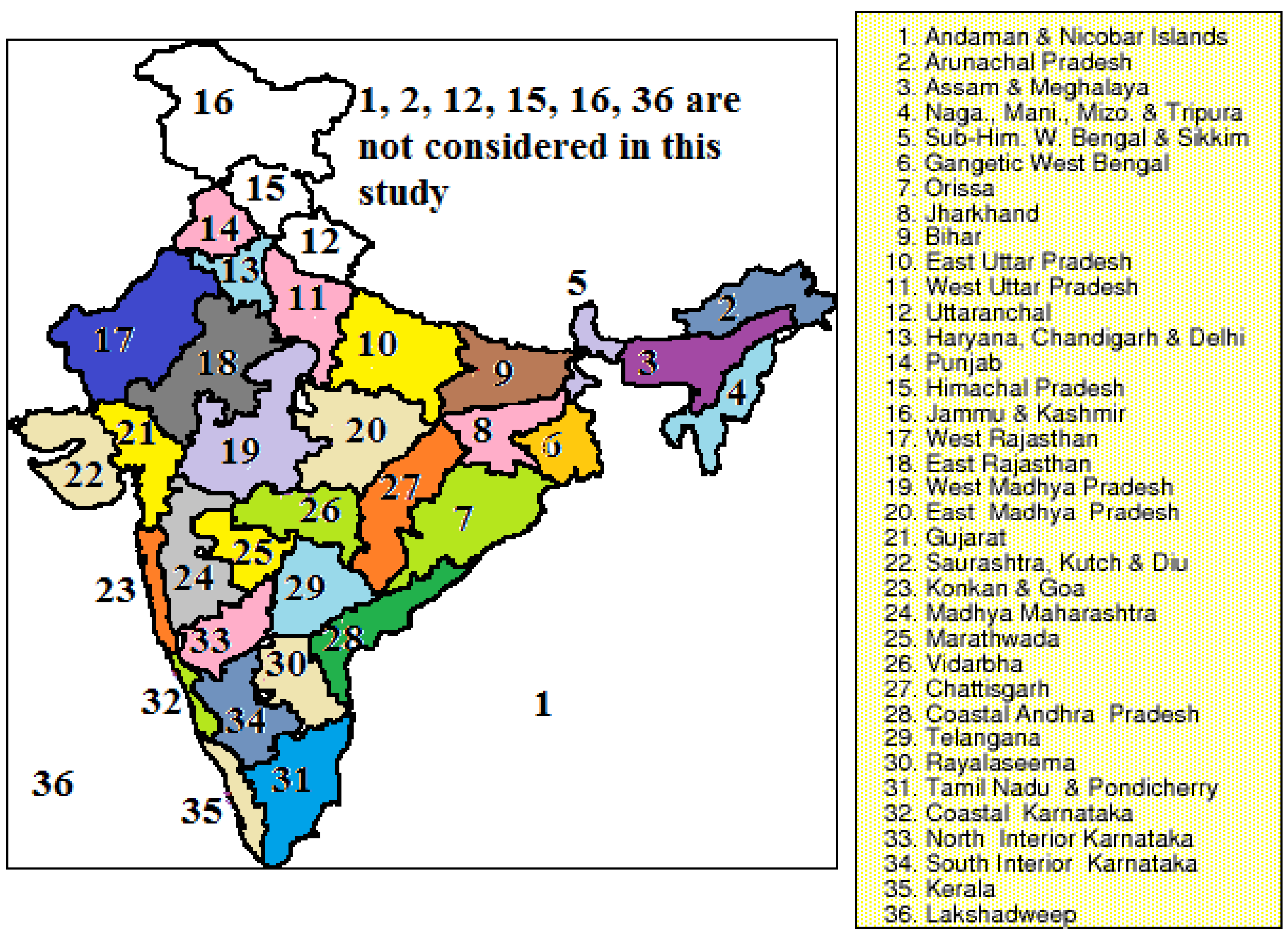
The data extraction included the development of a three-dimensional exhibit with the x, y, and z corresponding to longitude, latitude, and precipitation, respectively, for that specific month (in mm). The observed precipitation data have been taken from the website of the Indian Institute of Tropical Meteorology [17]. India is separated into 36 meteorological subdivisions. The insights about the meteorological subdivisions are given in Figure 1. The longitude and latitude values are utilized to separate the model data for comparing Indian meteorological subdivisions. Indian summer monsoon rainfall is considered from June to September, so it is defined as JJAS. Henceforth, for relative comparisons, all-India month-to-month precipitation is considered by taking the weighted average of 36 Indian meteorological subdivisions over JJAS, in view of their land secured. To distinguish models with a possibly sensible delineation of the monsoon rainfall, six measurable routines have been utilized and they are described as follows:

Figure 1. Details of Indian meteorological subdivisions.

Figure 1. Details of Indian meteorological subdivisions.

2.1. Z-Value Test

In statistics, the Z-value test or Z-test can be used to compare a sample mean with a reference mean, where distribution of the test statistic is defined as a difference between the two means divided by the standard deviation (std) of the observed and can be approximated by a normal distribution [18]. This statistic is calculated under the null hypothesis (H₀) that there is no statistical significant difference between model and the observed mean, and the alternative hypothesis (H₁) that there is a significant difference between model and the observed mean. Here, the Z-test is performed on the observed AISMR mean. The hypothesis is:

• H₀: μ = 848.63 mm/JJAS
• H₁: μ ≠ 848.63 mm/JJAS

It implies that models whose AISMR mean falls under a 95% confidence interval of normal distribution of observed mean rainfall (848.63 mm/JJAS) are accepted; others are rejected.

Out of those accepted models, the model possessing the lowest absolute Z-value will signify that the data associated with that particular model is almost similar to the observed data. Hence, that model will be accepted as the best model by this test.

2.2. Student’s T-Test

Here, Student’s t-test is used to find the significant difference between two samples (historical vs. projection) [19,20], where the hypothesis of the test is given below:

C.

$H_0:{\text{μ}}_2\le {\text{μ}}_1$

D.

$H_1:{\text{μ}}_2>{\text{μ}}_1$

where ${\mu }_1$ and ${\mu }_2$ are the mean of the historical and projected data (considered as sample mean). The null hypothesis is rejected at various confidence levels of 80%, 90%, 95%, and 99%.

2.3. Correlation Coefficient

This test is used to directly evaluate the similarity between the observed data and that provided by different models. It is defined as the covariance of the observed and the model divided by the product of their standard deviations. The test has been performed on subdivision means. The correlation coefficient is denoted by “r”. If r = 1, it implies a perfect positive linear correlation; if r = −1, it implies a perfect negative correlation; and r = 0 implies no linear relation between them (observed and models).

2.4. Relative Precipitation Comparison Test

In this test, mean rainfall of the model is directly compared with the observed mean. The observed mean is subtracted from each of the models and the result is divided by the observed mean. The formula used for getting the relative precipitation is given as:

$$Relative precipitation=\frac{\left(model mean-observed mean\right)}{observed mean}$$

(1)

2.5. Probability Density Function Comparison Test

We use Kolmogorov-Simrnov (K-S test) to find the statistical significant differences between observed and model probability distribution functions. The K-S statistic quantifies a distance between the empirical distribution function (EDF) of the sample (model) and the cumulative distribution function (CDF) of the reference distribution (observed) [21]. Here, the probability density function of each of the model is compared with the probability density function of the observed rainfall. The most accurate model is selected on the basis of values of statistics obtained from the K-S test. The minimum value of the K-S test signifies a best model. The null hypothesis is defined as:

$$H_0:d\left(ED{F}_{model},CD{F}_{obs}\right) \ne 0$$

$$H_1: d\left(ED{F}_{model},CD{F}_{obs}\right) = 0$$

where $d\left(ED{F}_{model},CD{F}_{obs}\right)$ implies the distance in between the EDF of the model and the CDF of the observation. The minimum value of the K-S statistics implies the distance between them is very small. The null hypothesis is rejected at the 95% confidence level.

2.6. Root Mean Square Error Test

The root mean square error or root mean square deviation (RMSD) test is frequently used to measure the difference between values predicted by a model (estimator) and the observed values. The output is indicative of the sample standard deviation of the differences between the predicted and observed values. It is calculated using the following formula:

$$RMSD = \sqrt{\frac{{{\displaystyle \sum }}_{t = 1}^n{\left(x_{1,t} - x_{2,t}\right)}^2}{n}}$$

(2)

where $x_{1,t}$ is the simulated rainfall while $x_{2,t}$ is the observed rainfall. The best model is the one with the least RMSE value.

3. TOPSIS Method for Ranking CMIP5 Models

TOPSIS is a multiple-attribute decision-making (MADM) technique which was first proposed by Hwang and Yoon [22,23]. TOPSIS implies that any given decision matrix with $m$ alternatives and $n$ attributes can be represented by points on an $n$-dimensional hyper-plane with $m$ points, with the location of these points being given by the value of their attributes. TOPSIS compares and ranks alternatives based on two sets of solutions known as the positive and negative ideal solutions. The ideal solutions are data-driven, i.e., the positive ideal solution contains data that are the most desirable from among all the alternatives and, similarly, the negative ideal solution contains data that are the least desirable from among all the alternatives. The ranking is determined by calculating the Euclidean distance of an alternative from these two ideal solutions. The alternative that has the largest distance from the negative solution and the smallest distance from the positive solution is termed as the best.

TOPSIS uses vector normalization for the scaling of data. TOPSIS is a very versatile and popular MADM tool among the scientific community. The TOPSIS method involves the following steps for a decision matrix having $m$ alternatives and $n$ attributes.

Step 1: Construction of normalized decision matrix.

$$r_{ij}= \frac{a_{ij}}{\sqrt{{{\displaystyle \sum }}_{i = 1}^m{\left(a_{ij}\right)}^2}} ; \forall j$$

(3)

Step 2: Construction of a weighted normalized decision matrix.

$$V_{ij} ={\left[r_{ij}\right]}_{m \times n}*{\left[W_j\right]}_{n \times n}^{diagonal}$$

(4)

Step 3: Determination of the positive ideal and negative ideal solution.

The positive ideal solution $V_j^{+}$ and the negative ideal solution $V_j^{-}$ are given by

$$V_j^{+}= \left\{\left(\max \left(V_{ij}, j\in J_1\right)\right),\left(\min \left(V_{ij},j\in J_2\right)\right), i = 1, 2, 3, \dots , m\right\}; \forall j$$

(5)

$$V_j^{-} = \left\{\left(\min \left(V_{ij}, j \in J_1\right)\right), \left(max \left(V_{ij},j\in J_2\right)\right), i = 1, 2, 3, \dots , m\right\}; \forall j$$

(6)

where $J_1$ and $J_2$ correspond to benefit criteria and cost criteria, respectively.

Step 4: Calculate the distances $d_i^{+}$and $d_i^{-}$ from the positive ideal and negative ideal solution, respectively.

$$d_i^{+}={\left\{{\displaystyle \sum }_{j = 1}^n{\left(V_{ij}-V_j^{+}\right)}^2\right\}}^{\frac{1}{2}} ; \forall i$$

(7)

$$d_i^{-} ={\{{\displaystyle \sum }_{j = 1}^n{\left(V_{ij}-V_j^{-}\right)}^2\}}^{\frac{1}{2 }} ; \forall i$$

(8)

Step 5: Determine the relative closeness of the alternatives to the ideal solution.

$$c{l}_i^{+} = \frac{d_i^{-}}{d_i^{+}+ d_i^{-}} ; \forall i$$

(9)

where $0 \le c{l}_i^{+} \le 1$. Alternatives with a higher magnitude of closeness are preferred.

4. Results and Discussion

In this study, information from the 20 CMIP5 models that have been utilized to analyze projected monsoon rainfall under the RCP 8.5 scenario was considered. These models have been contrasted with observed precipitation data for the historical time period of 1871–2005. Thus, to focus on possibly optimal models for precise future forecasts, the observed precipitation has been utilized as the comparison criteria. The observed AISMR mean is recorded to be 848.63 mm/JJAS with a standard deviation of 83.37 mm/JJAS.

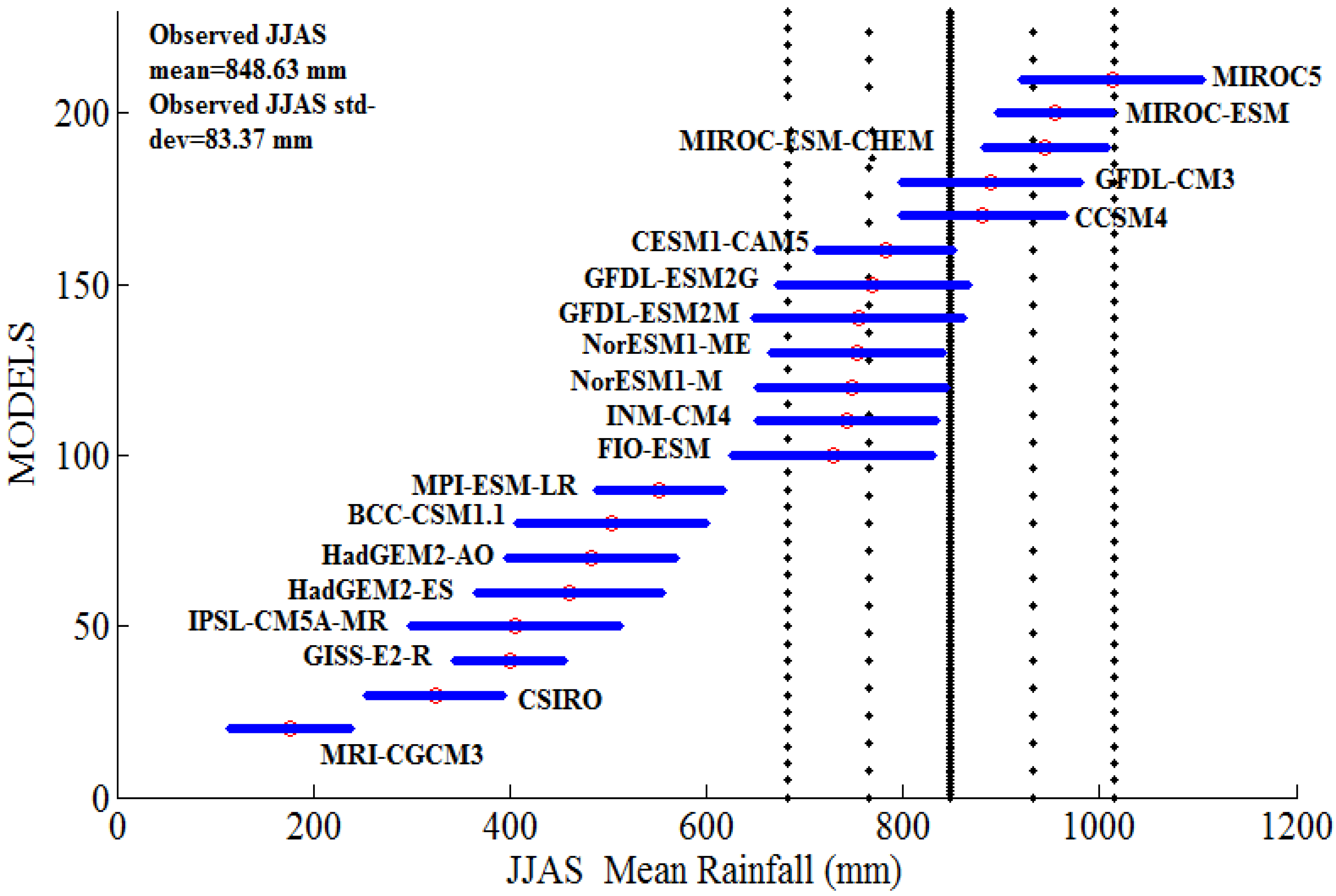
The statistical Z-test used for the purpose of evaluation has been discussed in the previous section. It can be observed from Figure 2 that the model CCSM4 has the closest proximity with the observed mean because it has the minimum Z-value. The Z-test values are listed in Table 2 for all 20 models. Moreover, it is seen from Figure 2 that models like MIROC, MIROC-ESM, MIROC-ESM-CHEM, GFDL-CM3, CCSM4, CESM1-CAM5, GFDL-ESM2G, GFDL-ESM2M, NorESM1-M, NorESM1-ME, INM-CM4, and FIO-ESM are within twice the standard deviation of the observed mean. Similar results were reported in [15].

Figure 2. AISMR mean from 20 models for the historic period of 1871–2005. The black vertical line shows the all-India mean monsoon rainfall from observations for the period of 1871–2005, and the dashed lines show the mean plus/minus one, and twice the standard deviation of the all-India mean rain. Circles with error bars represent mean and mean plus/minus one standard deviation for the 20 comprehensive models from 1871 to 2005.

Figure 2. AISMR mean from 20 models for the historic period of 1871–2005. The black vertical line shows the all-India mean monsoon rainfall from observations for the period of 1871–2005, and the dashed lines show the mean plus/minus one, and twice the standard deviation of the all-India mean rain. Circles with error bars represent mean and mean plus/minus one standard deviation for the 20 comprehensive models from 1871 to 2005.

The correlation coefficient test is used to find the linear relation between observed and model subdivisional mean. It is seen that the data of models CCSM4, CESM1-CAM5, MIROC5 and MPI-ESM-LR are linearly related with observations as they have the highest r values of 0.79, 0.77, 0.66, and 0.55, respectively, in comparison with other models.

The next test performed is a relative precipitation comparison and results for the same have been listed in Table 2. It is found that CCSM4, GFDL-CM3, CESM1-CAM5, and MIROC-ESM-CHEM are relatively close with the observation values as they have minimum errors. Also, it is seen that eight out of 20 models show a long-term positive trend in AISMR under the RCP 8.5 scenario at a 95% confidence level using Student’s t-test, which is depicted in Figure 3.

The two other tests performed are probability density function comparison and the root mean square error test. Figure 4 shows the results for probability density overlays. The K-S test statistic values, for which the hypothesis is accepted at the 95% confidence level, are listed in Table 2. Similarly, the root mean square error is calculated between the observed and model rainfall. The quantitative estimations of this test are listed in Table 2 and Figure 5.

Table 2. Quantitative values of the tests performed.

Models	Z-Value	RMSE Value (mm)	Relative Error	Cor. Coef	Pdf	Rank
CCSM4	0.3871	123.9	0.038	0.7965	0.1926	1
CESM1-CAM5	0.8034	136.5	0.0789	0.7750	0.3926	2
GFDL-CM3	0.4916	127.7	0.0485	0.4240	0.1778	3
GFDL-ESM2G	0.9472	144.8	0.0935	0.4240	0.3926	4
MIROC-ESM CHEM	1.1561	141	0.1136	0.4707	0.5259	5
NorESM1-ME	1.1387	161.4	0.1119	0.4229	0.4741	6
INM-CM4	1.2726	152.5	0.125	0.4403	0.4963	7
NorESM1-M	1.2069	163.2	0.1182	0.4159	0.4519	8
MIROC-ESM	1.2741	142.5	0.1252	0.4631	0.5778	9
GFDL-ESM2M	1.1271	165.7	0.1108	0.3458	0.4222	10
FIO-ESM	1.4313	186	0.1406	0.3521	0.4963	11
MIROC5	1.9597	205.1	0.193	0.6657	0.7037	12
MPI-ESM-LR	3.5579	317.2	0.3489	0.5519	0.963	13
BCC-CSM1.1	4.1368	369.9	0.4069	0.1804	0.9481	14
HadGEM2-AO	4.64	403.7	0.4565	0.5170	0.9556	15
IPSL-CM5A-MR	4.3746	382.4	0.4306	0.2710	0.9778	16
HadGEM2-ES	5.3117	461.4	0.5223	0.5013	0.9704	17
GISS-E2-R	5.3836	460.9	0.5293	0.2429	1	18
CSIRO	6.29	535	0.6184	0.4192	1	19
MRI-CGCM3	8.0679	680.1	0.792	0.4667	1	20

Table 2. Quantitative values of the tests performed.

Models	Z-Value	RMSE Value (mm)	Relative Error	Cor. Coef	Pdf	Rank
CCSM4	0.3871	123.9	0.038	0.7965	0.1926	1
CESM1-CAM5	0.8034	136.5	0.0789	0.7750	0.3926	2
GFDL-CM3	0.4916	127.7	0.0485	0.4240	0.1778	3
GFDL-ESM2G	0.9472	144.8	0.0935	0.4240	0.3926	4
MIROC-ESM CHEM	1.1561	141	0.1136	0.4707	0.5259	5
NorESM1-ME	1.1387	161.4	0.1119	0.4229	0.4741	6
INM-CM4	1.2726	152.5	0.125	0.4403	0.4963	7
NorESM1-M	1.2069	163.2	0.1182	0.4159	0.4519	8
MIROC-ESM	1.2741	142.5	0.1252	0.4631	0.5778	9
GFDL-ESM2M	1.1271	165.7	0.1108	0.3458	0.4222	10
FIO-ESM	1.4313	186	0.1406	0.3521	0.4963	11
MIROC5	1.9597	205.1	0.193	0.6657	0.7037	12
MPI-ESM-LR	3.5579	317.2	0.3489	0.5519	0.963	13
BCC-CSM1.1	4.1368	369.9	0.4069	0.1804	0.9481	14
HadGEM2-AO	4.64	403.7	0.4565	0.5170	0.9556	15
IPSL-CM5A-MR	4.3746	382.4	0.4306	0.2710	0.9778	16
HadGEM2-ES	5.3117	461.4	0.5223	0.5013	0.9704	17
GISS-E2-R	5.3836	460.9	0.5293	0.2429	1	18
CSIRO	6.29	535	0.6184	0.4192	1	19
MRI-CGCM3	8.0679	680.1	0.792	0.4667	1	20

Figure 3. Long-term trend in AISMR. Observations (black) are for the time period of 1871–2005 and model outputs (pink) are for the time period of 1871–2100.

Figure 3. Long-term trend in AISMR. Observations (black) are for the time period of 1871–2005 and model outputs (pink) are for the time period of 1871–2100.

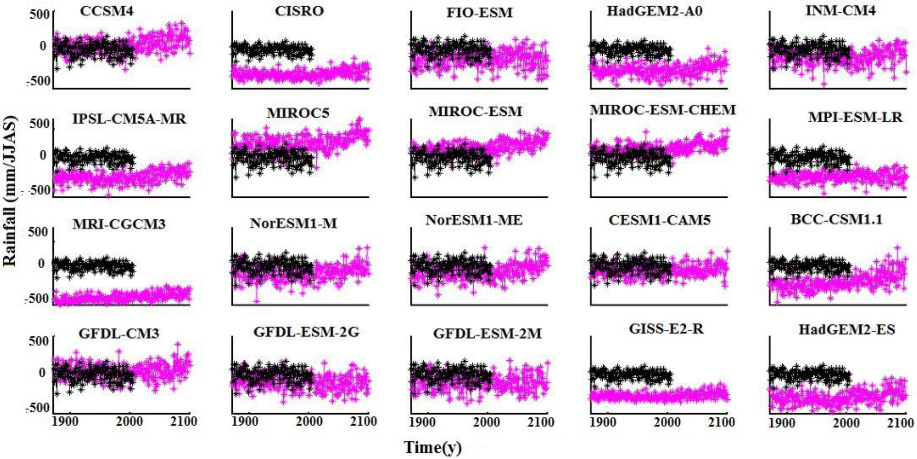
Figure 4. Probability density function for 20 models and observed data for AISMR. Black line represents observed data and red is for model data. The x-axis represents the precipitation of the models and the y-axis represents probability (in %).

Figure 4. Probability density function for 20 models and observed data for AISMR. Black line represents observed data and red is for model data. The x-axis represents the precipitation of the models and the y-axis represents probability (in %).

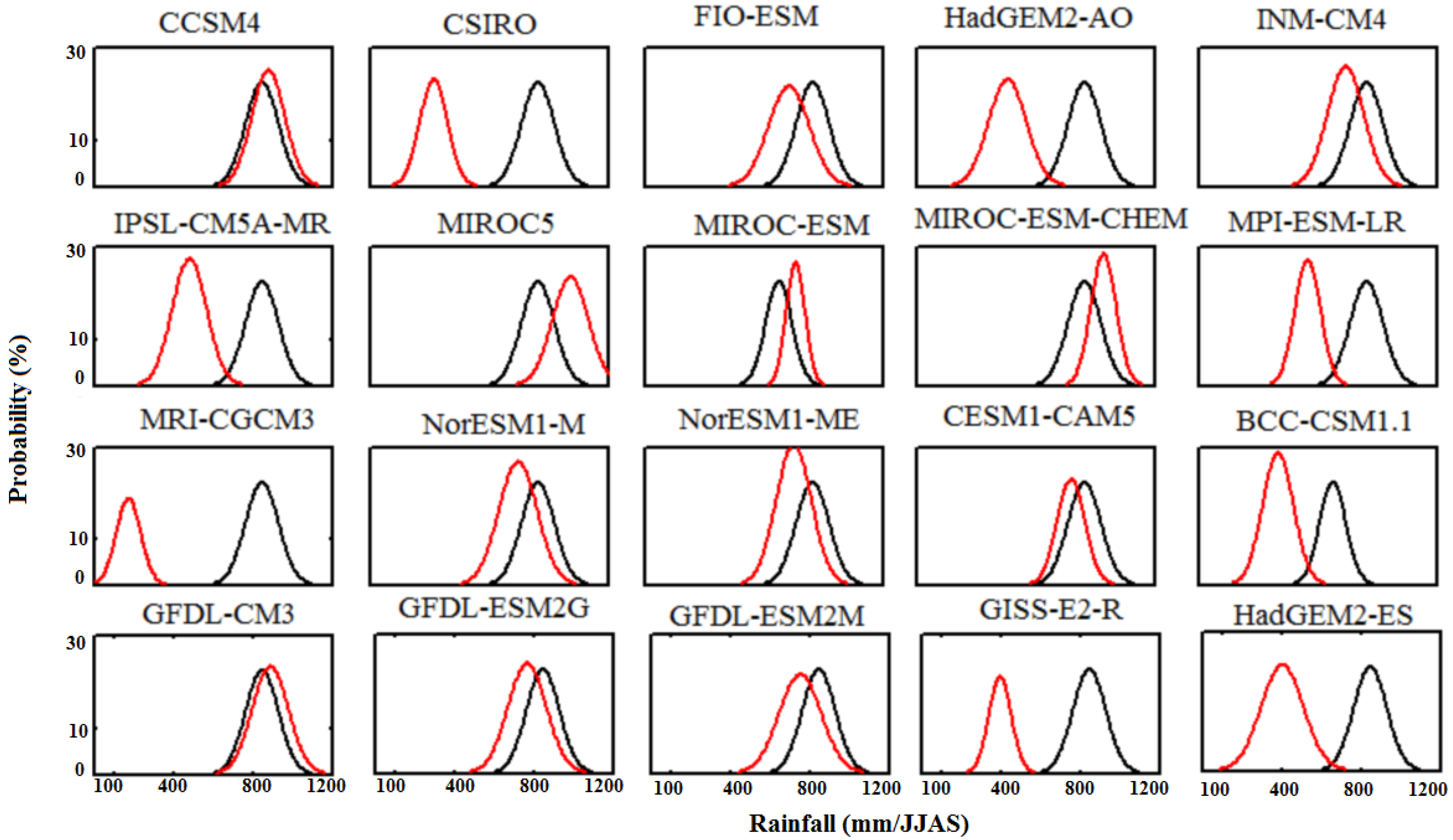
Figure 5. Root means square error between AISMR observed and models during 1871–2005.

Figure 5. Root means square error between AISMR observed and models during 1871–2005.

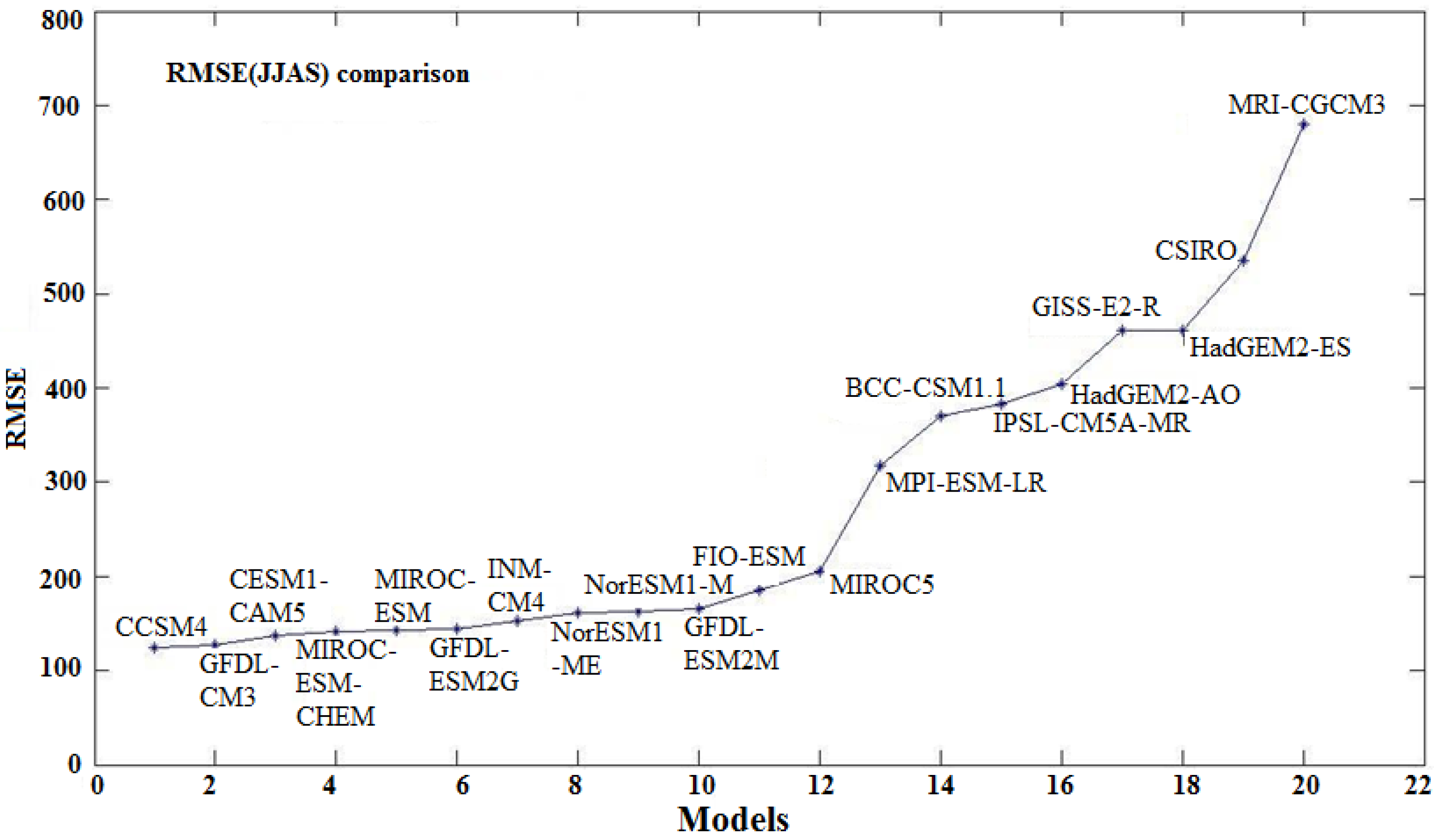
It is observed that some models behave well for only specific statistical tests. In order to get a suitable model, ranking is done using the TOPSIS method. In light of the models’ ranking it is found that CCSM4 is the best model for capturing the observed seasonal precipitation occurring over JJAS, trailed by three different models: CESM1-CAM5, GFDL-CM3, GFDL-ESM2G. TOPSIS ranking is given in Table 2.

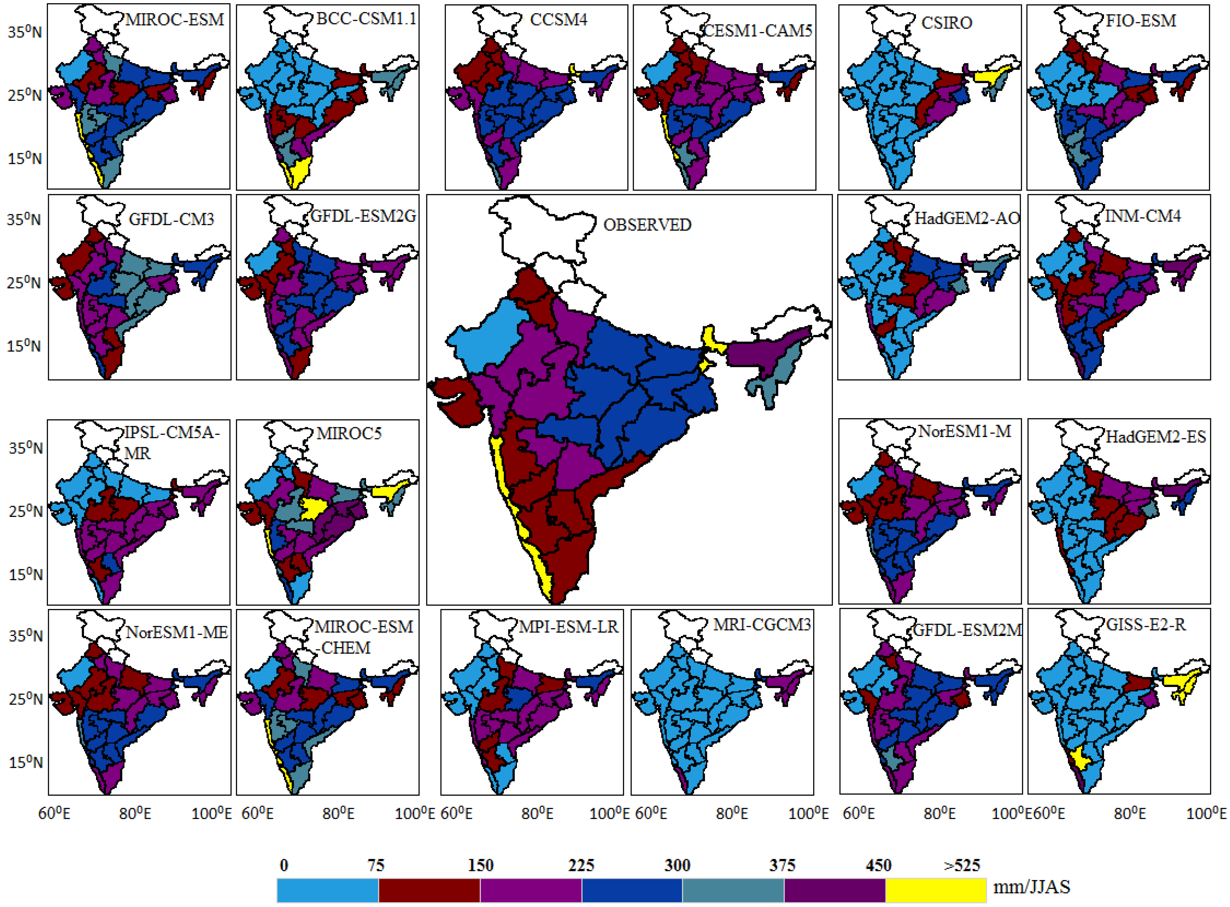
To check the closeness in spatial distribution, observed as well as model sub-divisional means are graphically depicted in Figure 6. The highest mean rainfall (more than 450 mm/JJAS) is observed over the southwest (Konkan and Goa, Coastal Karnataka, and Kerala) and the northeast (Sub-Himalaya, West Bengal, and Sikkim), and 375–450 mm/JJAS is observed in Assam and Meghalaya. Figure 6 shows that no model captures the spatial pattern completely; however, sub-divisional means of some of the models are very close to the observation.

Figure 6. Spatial patterns of JJAS mean rainfall across meteorological subdivisions of India over the time period 1871–2005.

Figure 6. Spatial patterns of JJAS mean rainfall across meteorological subdivisions of India over the time period 1871–2005.

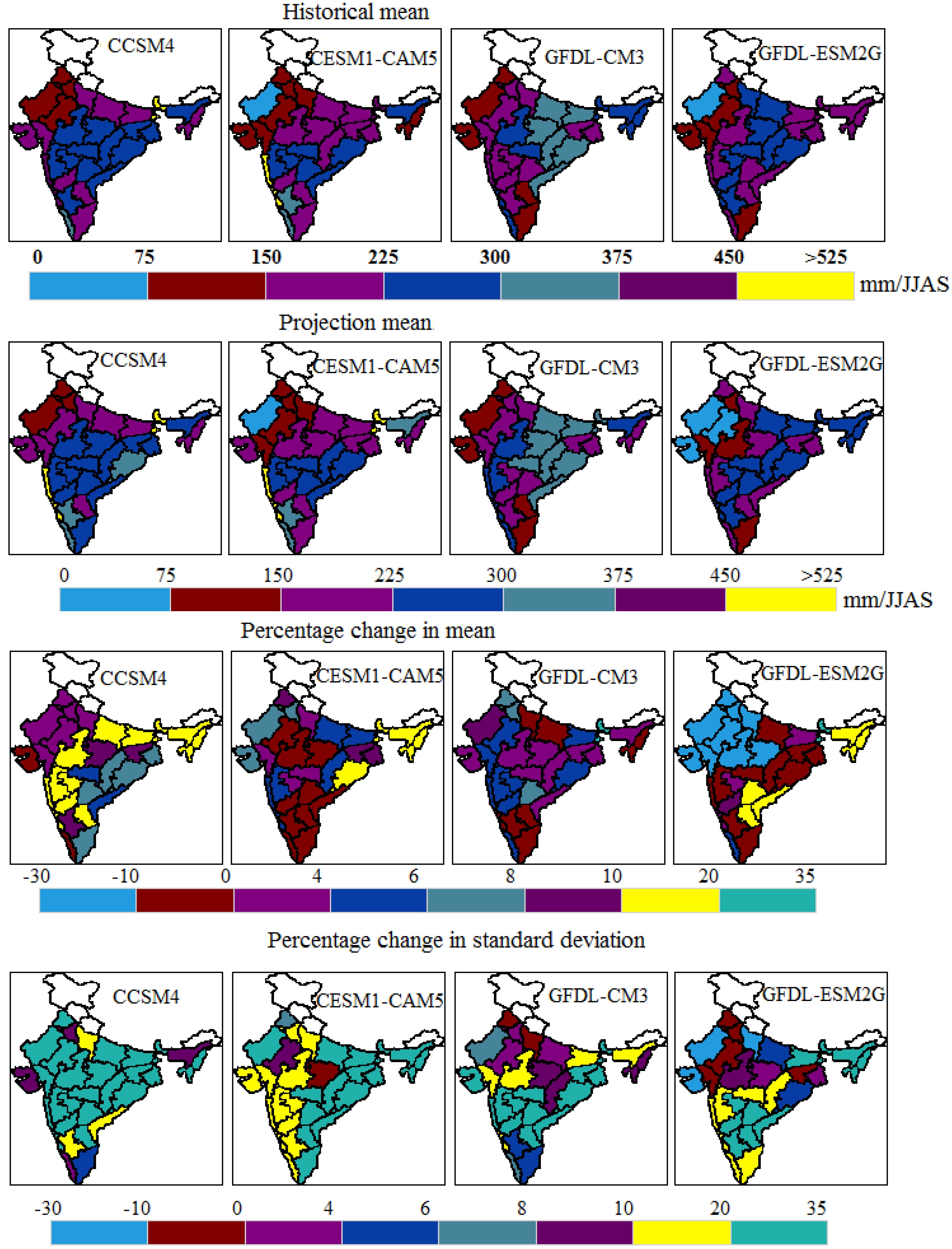
It is likewise imperative to notice the changes in the subdivisions of the optimum models. In Figure 7, maps compare the graphical patterns by means of four optimum models across meteorological subdivisions of India. The projection map predicts there is an increased rainfall in certain sub-divisions of India. Also, the percentage changes in the sub-divisional mean and standard deviation during the 21st century (2006–2100) with respect to the historic period (1871–2005) under RCP 8.5 are summarized in Figure 7. It is seen that these four optimum models do not show the same spatial patterns; however, a sub-divisional percentage change in mean for each model demonstrates in a comparable way. In the model CCSM4, it is seen from Figure 7 that subdivisions like Assam and Meghalaya, Bihar, East Uttar Pradesh, West Madhya Pradesh, Madhya Maharashtra, Konkan and Goa, Marathwada, North Interior Karnataka, Sub-Him, West Bengal and Sikkim, Nagaland, Manipur, Mizoram and Tripura, and Rayalaseema are liable to experience 10%–20% changes in mean rainfall. Similarly, the meteorological subdivisions such as West Uttar Pradesh, Coastal Andra Pradesh, and South Interior Karnataka are liable to encounter 10%–20% changes and the rest of the subdivisions are likely to experience 20%–35% changes in standard deviation. In comparison with CCSM4, it is seen that models CESM1-CAM5 and GFDL-ESM2G also show 10%–20% changes in mean in the northeast region. Thus, the chosen optimum models concur with the percentage changes in mean and standard deviation to some extent.

Figure 7. Comparison of the graphical patterns of means of four optimum models across meteorological subdivisions of India.

Figure 7. Comparison of the graphical patterns of means of four optimum models across meteorological subdivisions of India.

For AISMR, percentage changes are shown in Figure 8. The models are arranged in the order of their rank in Table 2. It is found that, on average, there will be a 10% change in mean and a 20% change in standard deviation (values are listed in Table 3). It is found that the relative increase in mean monsoon rainfall is up to 10% for the models that are within the range of two standard deviations from the observed mean, given in Figure 2. It is observed that in CCSM4, the future mean AISMR and standard deviation are likely to change by 8.2077% and 22.0146%, respectively. Similarly, in CESM1-CAM5, GFDL-CM3, and GFDL-ESM2G, the mean and standard deviation are likely to change by 2.8859, 17.0459; 2.1689, 13.4897; and −4.4374, 9.2692, respectively. It is found that model MRI-CGCM3 shows a maximum increase in mean AISMR of about 48.3% during the 21st century compared to the end of the 19th century for the RCP 8.5 scenario. From Figure 2, Figure 3, Figure 4 and Figure 5, it is seen that this model has maximum variation from the observations. Similar results were reported in [14]. In a similar manner, a maximum increase in standard deviation of about 58% is observed in model BCC-CSM1.1.

Figure 8. Percentage changes in mean and standard deviation of AISMR.

Figure 8. Percentage changes in mean and standard deviation of AISMR.

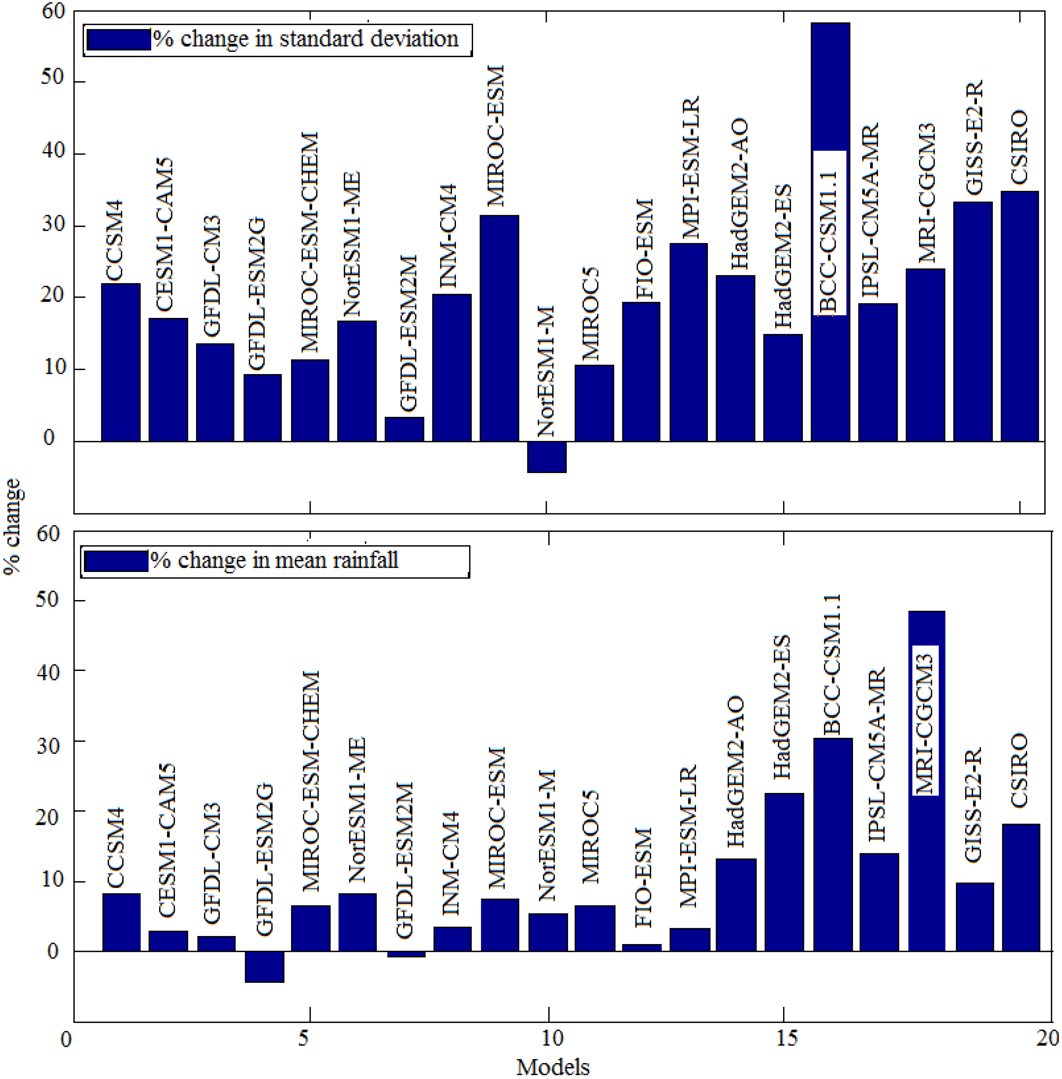
Table 3. Percentage changes in mean and standard deviation of AISMR for different models.

Models	Historical Mean (mm)	Historical Std (mm)	Projected Mean (mm)	Projected Std (mm)	Change in Mean (%)	Change in Std (%)
CCSM4	880.89	83.6526	953.1906	102.0684	8.2077	22.0146
CESM1-CAM5	781.6400	70.2667	804.1977	82.2443	2.8859	17.0459
GFDL-CM3	889.7600	91.6713	909.0578	104.0375	2.1689	13.4897
GFDL-ESM2G	769.2800	97.0605	735.1439	106.0572	−4.4374	9.2692
MIROC-ESM-CHEM	945.0700	63.5008	1007.1000	70.6841	6.5635	11.3121
NorESM1-ME	753.6800	88.8100	816.1367	103.6032	8.2869	16.6571
INM-CM4	742.5200	91.6529	768.5972	110.3688	3.5120	20.4204
NorESM1-M	748.3000	96.9179	787.7335	92.8092	5.2697	−4.2394
MIROC-ESM	954.8400	59.0414	1025.3000	77.6480	7.3792	31.5145
GFDL-ESM2M	754.5900	106.6198	748.5410	110.0879	-0.8016	3.2528
FIO-ESM	729.2900	102.9061	735.7116	122.7334	0.8805	19.2674
MIROC5	1012.4000	92.0586	1077.900	101.7629	6.4698	10.5414
MPI-ESM-LR	552.5200	64.7001	570.1562	82.4450	3.1920	27.4264
BCC-CSM1.1	503.7300	97.0290	656.2200	153.5000	30.2722	58.2001
HadGEM2-AO	461.2200	95.4294	522.0657	117.4652	13.1923	23.0912
IPSL-CM5A-MR	483.1900	86.8206	550.2872	103.4100	13.8863	19.1077
HadGEM2-ES	405.3700	106.5349	496.3961	122.4545	22.4551	14.9431
GISS-E2-R	399.4900	56.4887	438.7487	75.3044	9.8272	33.3088
CSIRO	323.8600	69.9287	382.8951	94.2486	18.2286	34.7781
MRI-CGCM3	176.5100	61.5337	261.9405	76.3110	48.3998	24.0150

Table 3. Percentage changes in mean and standard deviation of AISMR for different models.

Models	Historical Mean (mm)	Historical Std (mm)	Projected Mean (mm)	Projected Std (mm)	Change in Mean (%)	Change in Std (%)
CCSM4	880.89	83.6526	953.1906	102.0684	8.2077	22.0146
CESM1-CAM5	781.6400	70.2667	804.1977	82.2443	2.8859	17.0459
GFDL-CM3	889.7600	91.6713	909.0578	104.0375	2.1689	13.4897
GFDL-ESM2G	769.2800	97.0605	735.1439	106.0572	−4.4374	9.2692
MIROC-ESM-CHEM	945.0700	63.5008	1007.1000	70.6841	6.5635	11.3121
NorESM1-ME	753.6800	88.8100	816.1367	103.6032	8.2869	16.6571
INM-CM4	742.5200	91.6529	768.5972	110.3688	3.5120	20.4204
NorESM1-M	748.3000	96.9179	787.7335	92.8092	5.2697	−4.2394
MIROC-ESM	954.8400	59.0414	1025.3000	77.6480	7.3792	31.5145
GFDL-ESM2M	754.5900	106.6198	748.5410	110.0879	-0.8016	3.2528
FIO-ESM	729.2900	102.9061	735.7116	122.7334	0.8805	19.2674
MIROC5	1012.4000	92.0586	1077.900	101.7629	6.4698	10.5414
MPI-ESM-LR	552.5200	64.7001	570.1562	82.4450	3.1920	27.4264
BCC-CSM1.1	503.7300	97.0290	656.2200	153.5000	30.2722	58.2001
HadGEM2-AO	461.2200	95.4294	522.0657	117.4652	13.1923	23.0912
IPSL-CM5A-MR	483.1900	86.8206	550.2872	103.4100	13.8863	19.1077
HadGEM2-ES	405.3700	106.5349	496.3961	122.4545	22.4551	14.9431
GISS-E2-R	399.4900	56.4887	438.7487	75.3044	9.8272	33.3088
CSIRO	323.8600	69.9287	382.8951	94.2486	18.2286	34.7781
MRI-CGCM3	176.5100	61.5337	261.9405	76.3110	48.3998	24.0150

Lastly, it is imperative to demonstrate significant changes in mean at various confidence levels, as shown in Figure 9. We trust the results in Figure 9 are robust on the grounds that percentage changes that appeared in Figure 8 do not precisely demonstrate distinctions that are statistically significant. Here, we test a null hypothesis that there is no difference in mean rainfall between historical and projected data, which is rejected at various confidence levels against the alternate hypothesis that the projected mean is greater than the historical mean using a one-tailed two-sample t-test [20]. The consequences of Student’s t-test are given in Table 4.

Figure 9. Significant changes in mean at various confidence levels.

Figure 9. Significant changes in mean at various confidence levels.

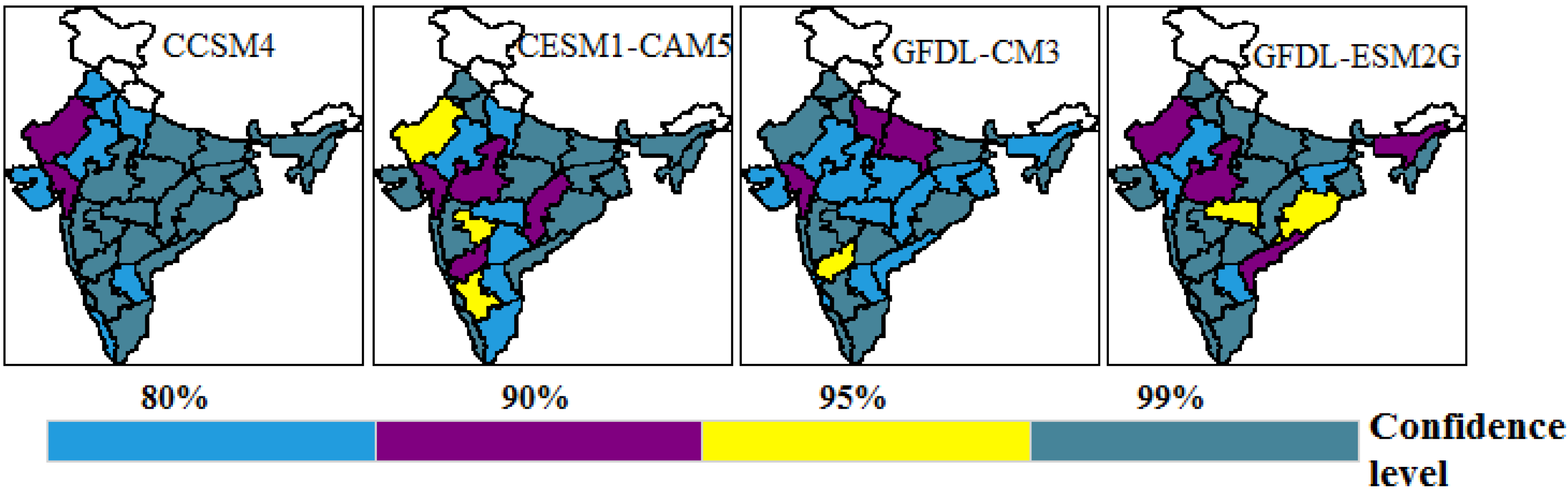
Table 4. Results of the t-test (the numbers in the first column represent meteorological subdivisions of the models mentioned in Figure 1).

Subdivisions Of Indian Region.	CCSM4H Value	CCSM4 Tstat Value	CESM1-CAM5 H Value	CESM1-CAM5 Tstat Value	GFDL-CM3 H Value	Tstat Value	GFDL-ESM2G H Value	Tstat Value
3	1	3.1918	0	−2.3054	0	0.3423	0	−4.0926
4	1	5.0288	0	−3.5458	1	2.8255	0	−4.1950
5	1	5.6283	0	−5.9594	0	−7.6830	0	−6.9997
6	1	2.4040	0	−2.9430	0	−0.4272	0	0.4418
7	1	2.1844	0	−3.3821	0	−1.6730	1	2.7121
8	1	3.3408	0	−2.7676	0	−0.1076	1	2.6312
9	1	3.1278	0	−1.2017	0	−1.8879	0	−0.7752
10	1	2.5083	0	−1.2557	0	0.8850	0	1.1680
11	0	0.1866	0	−0.1518	0	0.7660	1	5.8242
13	0	0.2579	0	−1.7960	0	−1.4831	1	5.5170
14	0	0.4851	0	−2.3072	0	−1.6966	1	4.7469
17	0	0.6212	0	−1.1210	0	−1.5813	1	4.5300
18	0	0.5435	0	−1.6183	0	−1.2329	1	5.3156
19	1	2.7873	0	−1.0441	0	−0.4740	1	3.2688
20	1	2.6581	0	1.2123	0	−0.0810	1	4.2279
21	0	0.7595	0	−0.8732	0	−0.8567	1	2.3534
22	0	−0.2848	0	−1.4930	0	−0.6006	1	2.1334
23	1	4.4458	0	−1.6183	0	0.8939	0	2.1334
24	1	3.6481	0	−1.0441	0	−1.2785	0	0.0221
25	1	3.6035	0	−0.0400	0	−1.0729	0	−0.6592
26	0	1.5056	0	−0.6453	0	−0.0717	0	1.1050
27	1	2.3492	0	−1.5515	0	−0.1111	0	1.36200
28	0	1.3216	0	1.3444	0	−0.0376	0	−2.9115
29	1	2.6522	0	0.5145	0	−1.5548	0	−3.1241
30	1	11.6299	0	0.2144	0	0.0838	0	−3.1855
31	1	2.7201	0	0.2096	0	1.2837	0	0.3814
32	1	4.4458	0	−1.6183	0	0.0086	0	−0.4567
33	1	4.9104	0	0.6908	0	−0.9744	0	−1.9052
34	1	3.5646	0	1.0849	1	2.4366	0	0.1630
35	0	−0.3084	0	1.4092	0	−2.5387	0	−1.0303

H—Represents either null hypothesis accepted or rejected. H = 1 implies null hypothesis is rejected, and it is accepted for H = 0.

Table 4. Results of the t-test (the numbers in the first column represent meteorological subdivisions of the models mentioned in Figure 1).

Subdivisions Of Indian Region.	CCSM4H Value	CCSM4 Tstat Value	CESM1-CAM5 H Value	CESM1-CAM5 Tstat Value	GFDL-CM3 H Value	Tstat Value	GFDL-ESM2G H Value	Tstat Value
3	1	3.1918	0	−2.3054	0	0.3423	0	−4.0926
4	1	5.0288	0	−3.5458	1	2.8255	0	−4.1950
5	1	5.6283	0	−5.9594	0	−7.6830	0	−6.9997
6	1	2.4040	0	−2.9430	0	−0.4272	0	0.4418
7	1	2.1844	0	−3.3821	0	−1.6730	1	2.7121
8	1	3.3408	0	−2.7676	0	−0.1076	1	2.6312
9	1	3.1278	0	−1.2017	0	−1.8879	0	−0.7752
10	1	2.5083	0	−1.2557	0	0.8850	0	1.1680
11	0	0.1866	0	−0.1518	0	0.7660	1	5.8242
13	0	0.2579	0	−1.7960	0	−1.4831	1	5.5170
14	0	0.4851	0	−2.3072	0	−1.6966	1	4.7469
17	0	0.6212	0	−1.1210	0	−1.5813	1	4.5300
18	0	0.5435	0	−1.6183	0	−1.2329	1	5.3156
19	1	2.7873	0	−1.0441	0	−0.4740	1	3.2688
20	1	2.6581	0	1.2123	0	−0.0810	1	4.2279
21	0	0.7595	0	−0.8732	0	−0.8567	1	2.3534
22	0	−0.2848	0	−1.4930	0	−0.6006	1	2.1334
23	1	4.4458	0	−1.6183	0	0.8939	0	2.1334
24	1	3.6481	0	−1.0441	0	−1.2785	0	0.0221
25	1	3.6035	0	−0.0400	0	−1.0729	0	−0.6592
26	0	1.5056	0	−0.6453	0	−0.0717	0	1.1050
27	1	2.3492	0	−1.5515	0	−0.1111	0	1.36200
28	0	1.3216	0	1.3444	0	−0.0376	0	−2.9115
29	1	2.6522	0	0.5145	0	−1.5548	0	−3.1241
30	1	11.6299	0	0.2144	0	0.0838	0	−3.1855
31	1	2.7201	0	0.2096	0	1.2837	0	0.3814
32	1	4.4458	0	−1.6183	0	0.0086	0	−0.4567
33	1	4.9104	0	0.6908	0	−0.9744	0	−1.9052
34	1	3.5646	0	1.0849	1	2.4366	0	0.1630
35	0	−0.3084	0	1.4092	0	−2.5387	0	−1.0303

H—Represents either null hypothesis accepted or rejected. H = 1 implies null hypothesis is rejected, and it is accepted for H = 0.

Figure 9 shows that subdivisions like Gujarat and West Rajasthan are liable to encounter 99% significant changes in mean, whereas subdivisions like Saurashtra, Kutch and Diu, Punjab, West Uttar Pradesh, Haryana, Chandigarh, Delhi, East Rajasthan, Rayalaseema, and Kerala are liable to experience 80% significant changes, and the rest of the subdivisions are liable experience 99% significant changes in mean according to model CCSM4.

Similarly, in other selected models, the subdivisions are liable to experience 80%–99% significant changes in mean.

5. Conclusions

This study investigates seasonal mean changes in AISMR and 30 meteorological subdivisions of India over the historical time period 1871–2005 and projected time period 2006–2100. We have found that the diverse models are fit for capturing distinctive parts of monsoon precipitation. These are the accompanying conclusions drawn from our study:

Using the multiple-attribute decision-making technique TOPSIS, we found that model CCSM4 (National Center for Atmospheric Research, USA) best fits the mean rainfall observations.

A few models catch the time-slice (seasonal) forecasts precisely, while the others have a superior spatial determination. Also, some different models still have fantastic concurrence with the observed data.

There is no all-inclusive answer for selecting the best model for a definite analysis. Consequently, it becomes indispensable to deliberately select the model that will yield precise forecasts relying upon the sort of examination required. In such a manner, this study is a first step to deliberately audit and select the ideal models for mean occasional expectation utilizing measurable methodologies.

Furthermore, this focus additionally gives us a chance to painstakingly audit and select the models for foreseeing geological circulation of the changing precipitation rates across the nation. This lends more believability and weight to the results provided in this study.

We look at the execution of models on AISMR and spatial patterns of subdivisions for the historical period of 1871–2005 from the precipitation data. From our examination we presume that four models, in particular CCSM4, CESM1-CAM5, GFDL-CM3, and GFDL-ESM2G, best catch the behavior of seasonal monsoon precipitation.

CCSM4 predicts an 8.2% change in AISMR mean precipitation which is roughly the average of different models, though CESM1-CAM5 and GFDL-CM3 foresee a 2% change in mean. Similarly, CCSM4 predicts a 22% change in standard deviation which is around average for the different models.

Recent study [16] has partitioned the CMIP5 models into unmistakable groups in light of the mean precipitation, seasonal cycle, and so forth. Furthermore, it is found that they reported that the group that indicates the highest reliability in projected changes in mean precipitation matches well with our four best models.

Subdivisions like Assam, Bihar Plains, East Uttar Pradesh., West Madhya Pradesh Madhya Maharashtra, Konkan and Goa, Marathwada, North Interior Karnataka, and Rayalaseema are prone to experience 10%–20% changes in mean precipitation, while subdivisions like Telangana, Orissa, Gangetic West Bengal, and Tamilnadu are liable to experience 20%–30% changes in mean precipitation, which is most astounding among all the subdivisions. The majority of these subdivisions show critical changes at the 99% confidence level (Figure 9).

In subdivisions such as Saurashtra and Kutch and Kerala, the mean precipitation is prone to diminish by 0%–10%, which indicates critical changes at the 80% confidence level (Figure 9). The diminishing mean precipitation in Kerala is a disturbing circumstance as this subdivision denotes the onset of an Indian summer monsoon.

References

- Intergovernmental Panel on Climate Change (IPCC). Climate Change 2013: The Science Basis Contribution of Working Group I to the Fifth Assessment Report of the Intergovernmental Panel on Climate Change; Cambridge University Press: New York, NY, USA, 2013; p. 1535. [Google Scholar]
- Sperber, K.R.; Annamalai, H.; Kang, I.S.; Kitoh, A.; Moise, A.; Turner, A.; Wang, B.; Zhou, T. The Asian summer monsoon: An intercomparison of CMIP5 vs. CMIP3 simulations of the late 20th century. Clim. Dynm. 2012, 41, 2711–2744. [Google Scholar] [CrossRef]
- Taylor, K.E.; Stouffer, R.J.; Meehl, G.A. An overview of CMIP5 and the experiment design. Bull. Amer. Meteor. Soc. 2012, 93, 485–498. [Google Scholar] [CrossRef]
- Turner, A.; Annamalai, H. Climate change and the South Asian summer monsoon. Nat. Clim. Change 2012, 2, 587–595. [Google Scholar] [CrossRef]
- Mahfouf, J.; Cariolle, D.; Royer, J.; Geleyn, J.; Timbal, B. Response of the Meteo-France climate model to changes in CO2 and sea surface temperature. Clim. Dynam. 1994, 9, 345–362. [Google Scholar] [CrossRef]
- Lal, M.; Cubasch, U.; Santer, B. Effect of global warming on Indian monsoon simulated with a coupled ocean-atmosphere general circulation model. Current sci. 1994, 66, 430–438. [Google Scholar]
- Timbal, B.; Mahfouf, J.; Royer, J.; Cariolle, D. Sensitivity to prescribed changes in sea surface temperature and sea ice in doubled carbon dioxide experiments. Clim. Dynam. 1995, 12, 1–20. [Google Scholar] [CrossRef]
- Lal, M.; Cubasch, U.; Voss, R.; Waszkewitz, J. Effect of transient increase in greenhouse gases and sulphate aerosols on monsoon climate. Current Sci. 1995, 69, 752–763. [Google Scholar]
- Meehl, G.A.; Washington, W.M. South Asian summer monsoon variability in a model with doubled atmospheric carbon dioxide concentration. Science 1993, 260, 1101–1104. [Google Scholar] [CrossRef] [PubMed]
- Kitoh, A.; Yukimoto, S.; Noda, A.; Motoi, T. Simulated changes in the Asian summer monsoon at times of increased atmospheric CO2. J. Meteor. Soc. Jpn. 1997, 75, 1019–1031. [Google Scholar]
- Lal, M.; Nozawa, T.; Emori, S.; Harasawa, H.; Takahashi, K.; Kimoto, M.; Abe-Ouchi, A.; Nakajima, T.; Takemura, T.; Numaguti, A. Future climate change: Implications for Indian summer monsoon and its variability. Current Sci. 2001, 81, 1196–1207. [Google Scholar]
- Cubasch, U.; Meehl, G.; Boer, G.; Stouffer, R.; Dix, M.; Noda, A.; Senior, C.; Raper, S.; Yap, K. Projections of future climate change. In Climate Change 2001: The Scientific Basis: Contribution of Working Group I to the Third Assessment Report of the Intergovernmental Panel; Houghton, J.T., Ding, Y., Griggs, D.J., Noguer, M., Van der Linden, P.J., Dai, X., Maskell, K., Johnson, C.A., Eds.; Cambridge University Press: Cambridge, UK, 2001; pp. 526–582. [Google Scholar]
- Fan, F.; Mann, M.E.; Lee, S.; Evans, J.L. Future changes in the south Asian summer monsoon: An analysis of the CMIP3 multi-model projections. J. Climate 2013, 25, 3909–3928. [Google Scholar] [CrossRef]
- Menon, A.; Levermann, A.; Schewe, J. Enhanced future variability during India’s rainy season. Geophys. Res. Lett. 2013, 40, 3242–3247. [Google Scholar] [CrossRef]
- Gadgil, S.; Sajani, S. Monsoon precipitation in the AMIP runs. Clim. Dynm. 1998, 14, 659–689. [Google Scholar] [CrossRef]
- Jayasankar, C.B.; Surendran, S.; Rajendran, K. Robust signals of future projections of Indian summer monsoon rainfall by IPCC AR5 climate models: Role of seasonal cycle and interannual variability. Geophys. Res. Lett. 2015, 42, 3513–3520. [Google Scholar] [CrossRef]
- Parthasarathy, B.; Munot, A.A.; Kothawale, D.R. Monthly and Seasonal Rainfall Series for All-India Homogeneous Regions and Meteorological Subdivisions: 1871–1994; Indian Institute of Tropical Meteorology: Pune, India, 1995. [Google Scholar]
- Crow, E.L.; Davis, F.K.; Maxfield, M.W. Statistical Manual: With Examples Taken from Ordnance Development; Dover: Mineola, NY, USA, 1961. [Google Scholar]
- Sprinthali, R.C. Basic Statistical Analysis, 9th ed.; Pearson Education: Boston, MA, USA, 2011. [Google Scholar]
- O’mahony, M. Sensory Evaluation of Food: Statistical Methods and Procedures; CRC Press: Boca Raton, FL, USA, 1986; p. 487. [Google Scholar]
- Massey, F.J. The Kolmogorov-Smirnov test for goodness fit. J. Am. Stat. Assoc. 1951, 46, 68–78. [Google Scholar] [CrossRef]
- Yoon, K.P.; Hwang, C.L. Multiple Attribute Decision Making: An Introduction; Sage Publications: Thousand Oaks, CA, USA, 1995. [Google Scholar]
- Lai, Y.J.; Liu, T.Y.; Hwang, C.L. Topsis for MODM. Eur. J. Oper. Res. 1994, 76, 486–500. [Google Scholar] [CrossRef]
© 2015 by the authors; licensee MDPI, Basel, Switzerland. This article is an open access article distributed under the terms and conditions of the Creative Commons Attribution license (http://creativecommons.org/licenses/by/4.0/).