Seasonal and Spatial Variation of Surface Urban Heat Island Intensity in a Small Urban Agglomerate in Brazil

Abstract

In recent years, SUHIs (surface urban heat islands) have been greatly emphasized in urban climate studies, since it is one of the climate phenomena most influenced by human action. In this study, temporal and spatial variations of SUHIs in the cities of Ceres and Rialma (Brazil) were investigated; satellite Landsat 8 TIRS/OLI images from 2013 to 2016 were used for this purpose. The results showed that in all seasons, two relationships were observed, one positive and one negative. An $NDVI$ (Normalized Difference Vegetation Index) of 0.2 is the divider of this relationship: up to this value, the relationship is positive, that is, the higher the $NDVI$ value, the higher the surface temperature, while the relationship is negative at an $NDVI$ greater than 0.2. There was high seasonal variation in the SUHIs, with the highest intensities recorded in the spring and summer (±12 °C), and the lowest in the winter. These temporal variations were attributed to the annual cycle of precipitation, which directly involves the robustness of the Cerrado vegetation. SUHIs occupied, on average, an area three times larger than the area of SUCIs (surface urban cool islands). The highest values of SUCIs were observed in water bodies and in valley bottoms. Overall, SUHIs showed high intensities; however, a more intense core area, such as in large cities, was not observed.

1. Introduction

Rapid and unplanned urban growth results in a continuous increase in land use, defined as the conversion of open spaces into artificial surfaces as well as green urban areas and sporting and leisure facilities [1].

The land surface temperature (LST) is an important indicator for quantifying urban heat islands (UHIs) and surface urban heat islands (SUHIs). UHIs have been regarded as the most well-documented example of anthropogenic climate modification within the field of urban climate [2,3].

The UHI phenomenon describes the excess warmth of the urban atmosphere and surfaces compared to non-urbanized rural surroundings. In general, three types of heat islands are recognized: (A) the canopy layer heat island; (B) the boundary layer heat island, and (C) the surface urban heat island. The first two types are atmospheric heat islands produced by urbanization. Both refer to a warming of the urban atmosphere [4]. A surface urban heat island (SUHI) refers to the relative warmth of the urban surfaces compared to their non-urbanized surroundings [4,5,6]. In contrast, the term surface urban cool island (SUCI) is defined as an urban area where lower surface temperatures prevail compared to non-urbanized dry surroundings.

SUHIs can be controlled by numerous factors, the most important of which are the modification in radiation balance, the emission of anthropogenic heat, the reduction in evapotranspiration from vegetation and soils, thermal accumulation in buildings and pavements and the reduction of average wind speed [2,7].

The adverse effects of UHIs include: (A) increasing thermal discomfort; a UHI will increase the duration and the degree of thermal discomfort [8]; (B) air pollution; a UHI increases the production of ozone near the ground [9] and, in the form of mesoscale wind, dispersed air pollution [10]; (C) increase in energy consumption [11]; (D) reduction in water quality; rapid temperature changes in water ecosystems caused by surface runoff from hot pavements and roofs covered with asphalt, mostly stressful and fatal for aquatic life [12]; and (E) increase in per capita water consumption in summer time [13].

Thus, greater knowledge of the thermal consequences of sealed soils could be very useful for urban planners and land-use decision makers for promoting an efficient soil sealing management approach in urban environments. Therefore, the objective of this work was to analyze the seasonal and spatial variation of the surface urban heat island intensity in a small urban agglomerate in Brazil.

2. Materials and Methods

2.1. Study Area

The population in the urban core of the cities of Ceres and Rialma was 31,245 inhabitants in 2014 [14]. The municipality of Ceres has twice the population of Rialma, but Rialma has a municipal area greater than Ceres. The relief of the region is uneven with steep slopes, surrounded by valleys and hills. As seen in Figure 1, the two cities are separated by the Rio das Almas, which features two well-defined regimes (a full regime and an ebb regime). Ceres streets are wide, while in Rialma, they are narrower.

Ceres is a city known regionally for its services in health and education. Ceres and Rialma have an interdependent relationship of working-housing. Therefore, the landscape of Ceres/Rialma is a dimension of the social relationships that are established in the city and region, i.e., it is the result of the social relationships of production and domination that are established there.

2.2. Data

The Landsat sensors have been monitoring the Earth for more than four decades, providing a continuity of data thoughout their lifetime [15]. The first series of these satellites was launched in 1972 and it was named the Earth Resources Technology Satellite; it was later renamed to Landsat 1. Since then, there has been a total of 8 Landsat satellites. Among the eight, Landsat 6 failed to attain orbit and fell to Earth in 1993. The remaining satellites have proven to be successful and have provided researchers with massive volumes of data which have been used in many studies [15,16]. Landsat data are freely available to download from the United States Geological Survey (USGS) website [17].

Table 1. Landsat 8 TIRS/OLI scenes used in this study.

Date	Time (UTC)	Path	Row	Cloud Cover
18 June 2013	13:22	222	071	0.01
5 August 2013	13:22	222	071	0.00
24 October 2013	13:22	222	071	0.01
4 May 2014	13:20	222	071	0.01
21 June 2014	13:20	222	071	0.01
8 August 2014	13:20	222	071	0.00
9 September 2014	13:21	222	071	0.01
31 January 2015	13:20	222	071	0.02
10 July 2015	13:20	222	071	0.01
11 August 2015	13:20	222	071	0.01
14 October 2015	13:20	222	071	0.01
23 April 2016	13:20	222	071	0.02
10 June 2016	13:20	222	071	0.01
12 July 2016	13:20	222	071	0.01

shows the Landsat scenes used in the study.

The methodology in this study is divided into sub-algorithms, which are sequentially presented in the next subsections.

2.3. Estimation of SUHIs

The calculation of the surface urban heat islands was carried out in six steps: The first was the conversion of digital numbers into radiance; the second was the calculation of the brightness temperature; the third was the calculation of the $NDVI$; the fourth consisted of estimating the surface soil emissivity from the $NDVI$ values obtained; and the fifth step, after the emissivity was estimated, consisted of determining the corrected surface temperature, which was subsequently converted into the surface urban heat island in the sixth step, as suggested by [15].

2.3.1. Step 1—Conversion of Digital Numbers (DN) to Radiance

The thermal data in satellite imagery of Landsat sensors are stored in digital numbers (DN). Digital numbers are used as a way of representing pixels that have not yet been calibrated. They are a representation of the different levels of radiance in the raster image. After obtaining the satellite images, the first step was the conversion of digital numbers into radiance. Equation (1) shows the equation used to convert DN into spectral radiance [18] of the Landsat 8 satellite TIRS sensor.

$$L_{\lambda }=M_L\times Q_{cal}+A_L-O_i$$

(1)

where $L_{\lambda }$ is the spectral radiance in $W/(m^2\times sr\times \mu m)$ at the top of the atmosphere. $M_L$ is the band-specific multiplicative rescaling factor from the metadata (radiance_mult_band_10). $Q_{cal}$ is the quantized and calibrated standard product pixel values (DN). $A_L$ is the band-specific additive rescaling factor from the metadata (radiance_add_band_10). $O_i$ are the corrections published by USGS for calibration of the TIRS bands.

2.3.2. Step 2—Computation of Brightness Temperature (BT)

The brightness temperature was calculated by Equation (2).

$$BT\frac{K_2}{\ln \left(\frac{K_1}{L_{\lambda }}+1\right)}$$

(2)

where $BT$ is the brightness temperature in (K), $L_{\lambda }$ is the spectral radiance at the top of the atmosphere, $K_1$ and $K_2$ is a specific constant for conversion into the thermal band.

2.3.3. Step 3—Calculation of $NDVI$

The normalized difference vegetation index ($NDVI$) is a simple graphical indicator that can be used to analyse remote sensing measurements, typically from satellite image data, and assess whether the target being observed contains live green vegetation. Consequently, we also explored the transformation of $NDVI$ into values associated with cover fraction using empirical relationships with vegetation indices, as a possible basis function. The Normalized Difference Vegetation Index ($NDVI$) is given by:

$$NDVI=\frac{L_{\lambda }\left(NIR\right)-L_{\lambda }\left(R\right)}{L_{\lambda }\left(NIR\right)+L_{\lambda }\left(R\right)}$$

(3)

where $NDVI$ is the Normalized Difference Vegetation Index. $NIR$ is the near infrared band and $R$ is the red band.

2.3.4. Step 4—Determination of Land Surface Emissivity (LSE)

The Land Surface Emissivity was estimated from the $NDVI$ values. According to [19], when the $NDVI$ of an area is known, the LSE can be estimated. The LSE of a pixel is estimated by classifying the pixels according to the class that they fall into. When a pixel has an $NDVI$ value that is below −0.185, then the LSE value of 0.995 is assigned to the pixel; when the $NDVI$ value is greater than or equal to −0.185 and is less than 0.157, an LSE value of 0.985 is assigned to the pixel, when the $NDVI$ value is greater than or equal to 0.157 and is less than or equal to 0.727, a logarithmic relationship between $NDVI$ and LSE is used [15], and finally, when the $NDVI$ value is greater than 0.727, the pixel is assigned a value of 0.990, as shown in

Table 2. Algorithm based on the $NDVI$ image.

$\mathit{N}\mathit{D}\mathit{V}\mathit{I}$	LSE
$NDVI<-0.185$	0.995
$-0.185\le NDVI<0.157$	0.985
$0.157\le NDVI\le 0.727$	$1.009+0.047\times \ln \left(NDVI\right)$
$NDVI>0.727$	0.990

.

2.3.5. Step 5—Correction of Land Surface Temperature (LST)

After estimating the soil surface emissivity, brightness temperature correction was performed. For this, Planck’s function was used. Equation (4) shows Planck’s function [20,21]. This function corrects the emissivity of a surface, in comparison to a black body.

$$LST=\frac{BT}{\left\{1+\left[\frac{\lambda \times BT}{\rho }\right]\times \ln \epsilon \right\}}$$

(4)

where $LST$ is the surface temperature (K), $BT$ is the brightness temperature (K), $\lambda$ is the wavelength of the emitted radiation, $\rho$ is $\left(h\times c÷\sigma \right)=1.438\times {10}^{-2} \mathrm{mK}$: $h$ is Planck’s constant ($6.26\times {10}^{-34}$ Js); $c$ is the velocity of light ($2.998\times 108 \mathrm{m}/\mathrm{s}$); $\sigma$ is Stefan Boltzmann’s constant ($1.38\times {10}^{-23} {\mathrm{J}·\mathrm{K}}^{-1}$) and $\epsilon$ is the surface emissivity.

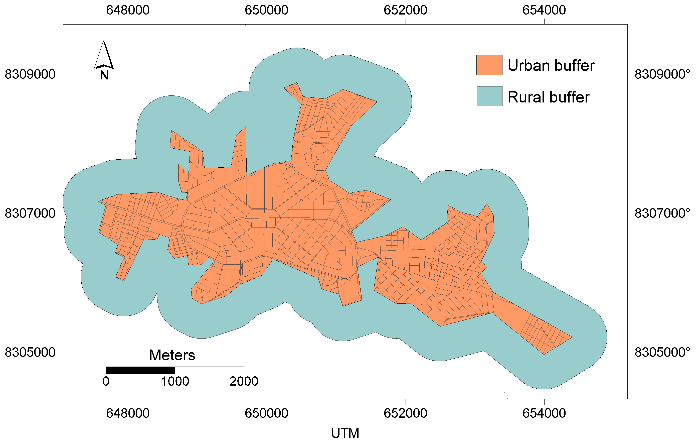
2.3.6. Step 6—Transformation of LST into the Surface Urban Heat Islands

To calculate the SUHIs, two buffers were produced, one rural, one urban. The rural buffer is located 500 m from the urban buffer (Figure 2).

Usually, the urban heat island (UHI) intensity is measured from observations of the air temperature along transects or in fixed stations in the urban and surrounding rural areas [22,23]. Nonetheless, the SUHI has another meaning; therefore, SUHI was calculated as the difference between the surface temperature of each pixel of the buffer in the urban area and the average surface temperature of the buffer in the rural area [5,24], according to Equation (5), shown in Figure 2.

$$SUHI=LS{T}_U-LS{T}_R$$

(5)

where $LS{T}_U$ is the surface temperature of the buffer urban and LST is the surface temperature of the buffer rural area. A positive value represents an SUHI situation, while a negative result represents a SUCI.

3. Results and Discussion

3.1. Seasonal Characteristics of the SUHIs

Seasonality of the SUHIs has been observed in several cities: in Tehran (Iran) [25], in Szeged (Hungary) [26] and in Erbil (Iraq) [27].

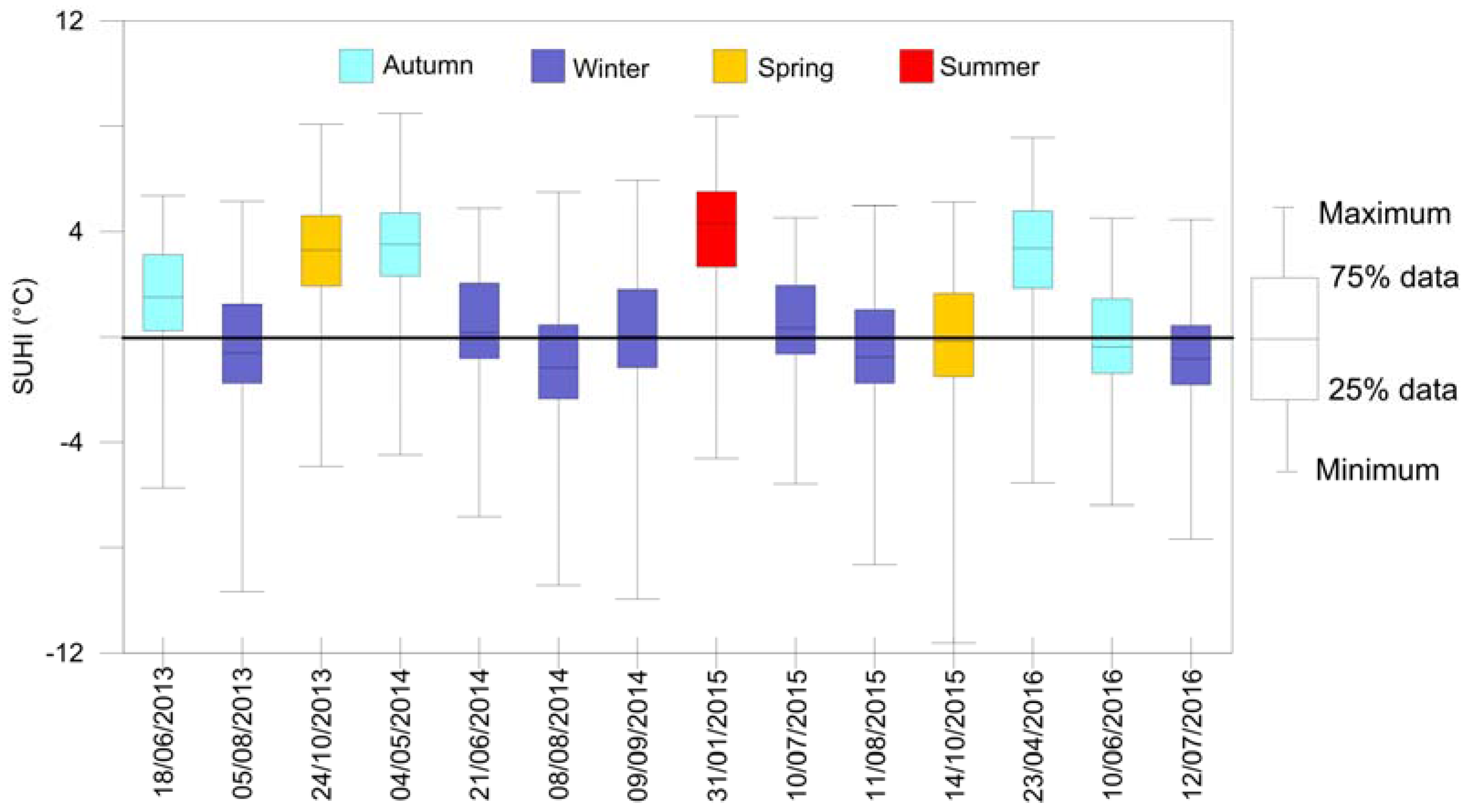
In Ceres-Rialma, the seasonality was evident, as shown in Figure 3 and Figure 4. In the winter, the intensity of SUHI was lower than in other seasons. The highest intensities of the SUHIs occurred in the summer, i.e., 12 °C. In autumn and spring, there was a significant time difference between the SUHI values.

The highest amount and intensity of the negative SHUIs, also called the surface urban cool islands (SUCIs), was observed in winter. SUHI bloxplots (Figure 3) contained all data presented in Figure 4, and therefore not only represent the urbanized area but also the rural area.

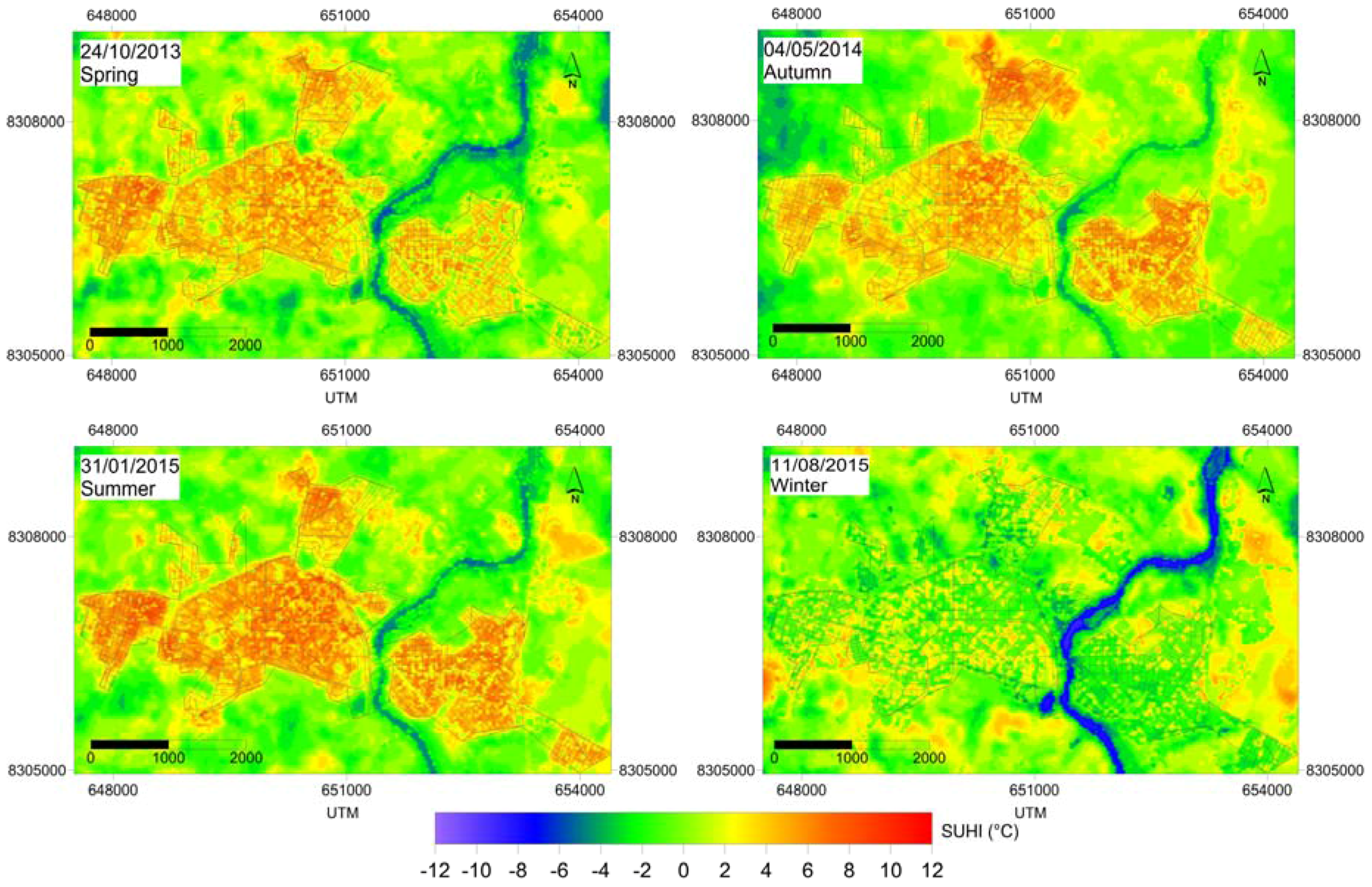
The seasonal variation in the SUHIs (Figure 4) is likely to result from the change in the intensity of solar radiation due to the movement of the Earth and the variation in the Cerrado vegetation and pastures, according to the rainfall [28].

The highest intensities in the SUHIs were observed in the summer (31 January 2015), a time that corresponds to the rainy season in the region, where the vegetation and pasture become more dense with increased metabolic activity. At this time, the contrast between urban and rural areas is higher, and therefore, the intensities of the SUHIs tend to be higher. By contrast, in the winter (11 August 2015), there was little difference in the intensity of the SUHIs of the urban area compared to the SUHIs of the rural area, as in this period, the Cerrado vegetation and pastures dry out or lose their leaves to minimize the adverse effects of the lack of precipitation.

3.2. Spatial Characteristics of the SUHIs

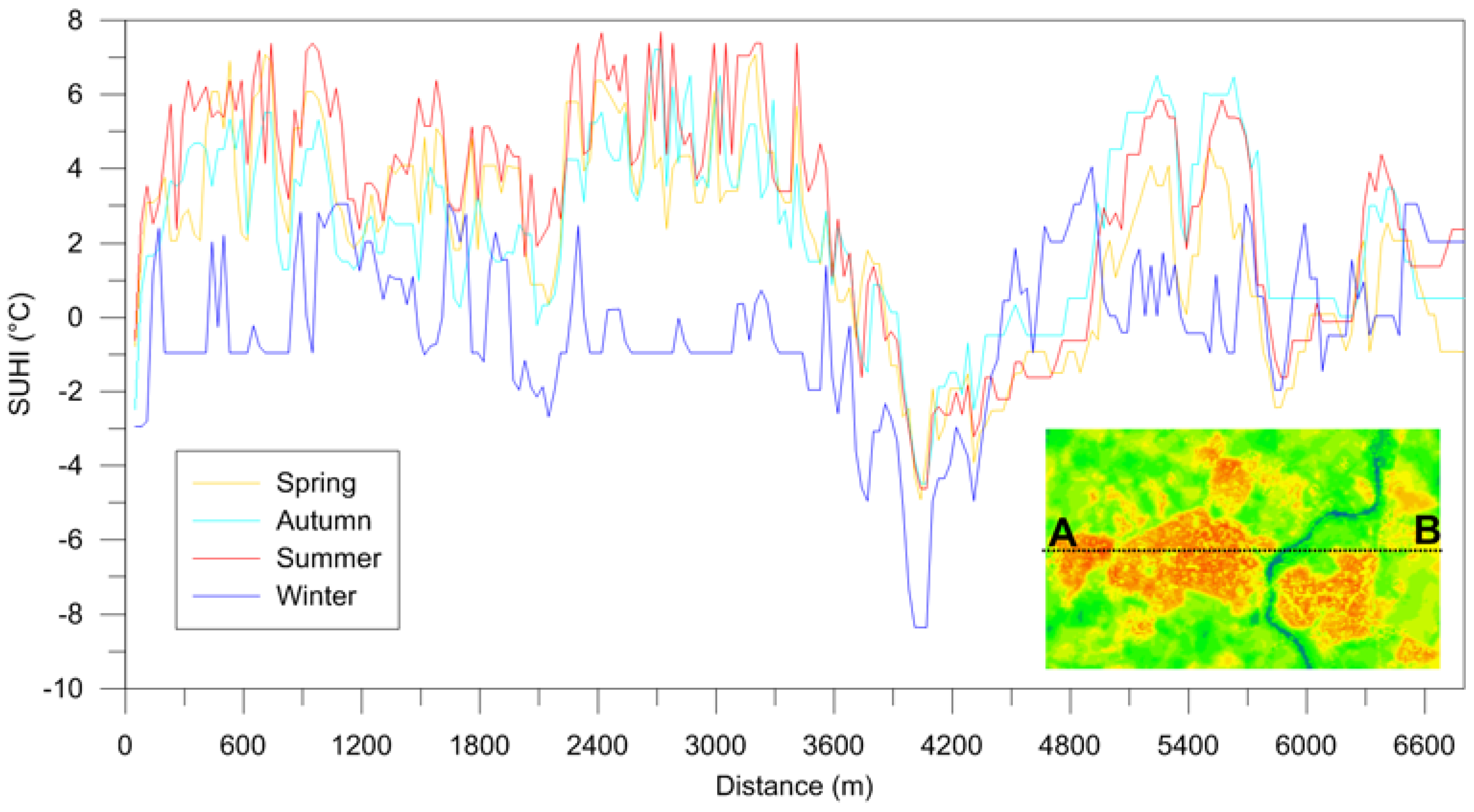
In order to analyze the temporal and spatial variation of the average intensity of the SUHIs, a transect from point A to point B (Figure 5) was established, with a regular distance of 30 m, totaling 225 data points. The profile of Figure 5 shows the influence of different types of land use and occupation on the intensity of the SUHIs; initially, in the first few meters of the transect, SUHIs close to 8 °C were observed in the summer. Between 1200 and 1900 m, lower intensities were measured. From the point of 3600 to 4600 m, lower intensities of the SUHIs were observed in all seasons. This occurred because this space is outside the urban boundary, encompassing vegetation sites and the Rio das Almas.

It can be noted in Figure 5 that in almost all transects in winter, the intensities of the SUHIs were lower than in other seasons, while in the summer, most SHUIs had the highest intensities. The spatial variation of the SUHIs in the autumn and spring had similar patterns. Therefore, there is a sharp contrast, especially in the summer and winter seasons, in the intensity of SUHIs in the urban agglomerate of Ceres-Rialma.

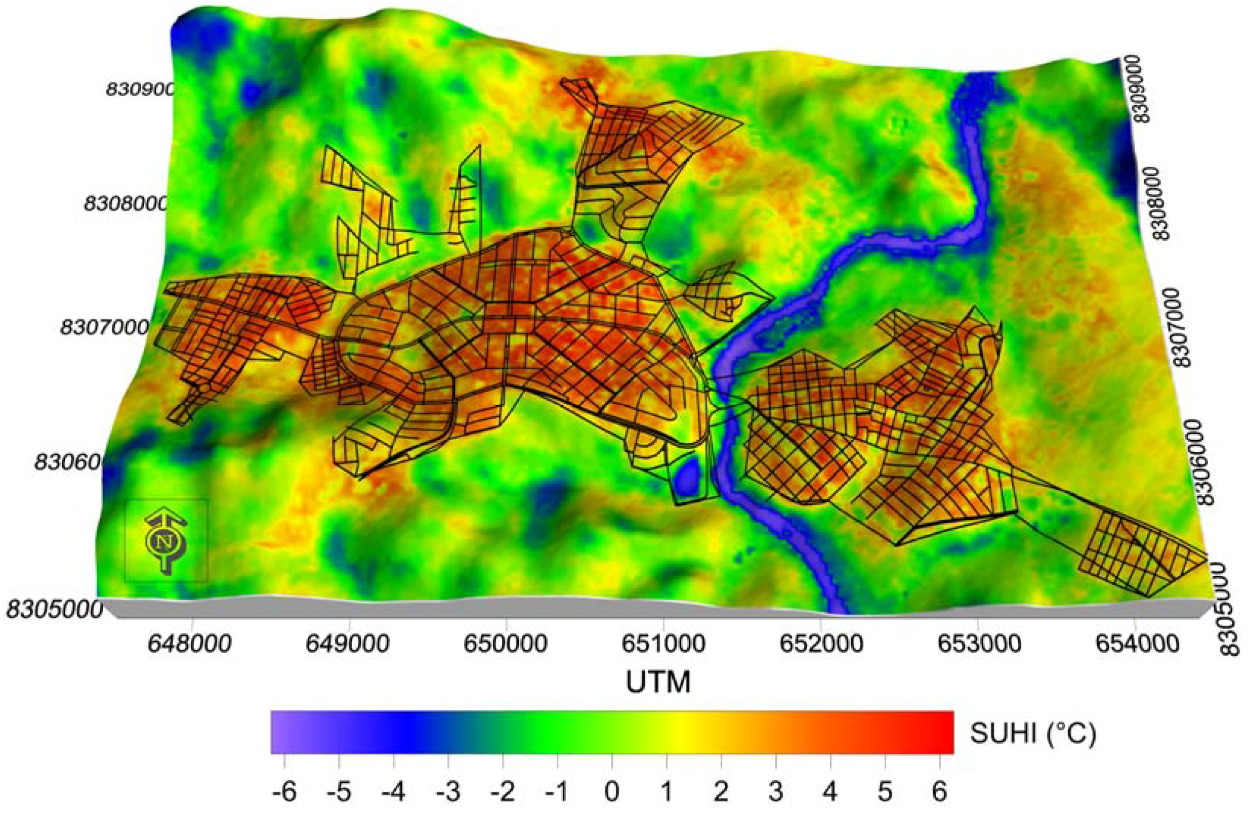
The average SUHIs superimposed on the relief (Figure 6) enable one to check that valley bottom areas or steep slope areas showed the highest intensities of the SUCIs. Rio das Almas, which divides the cities of Ceres and Rialma, has lower intensities due to the heat capacity of water and the lower intensity of solar radiation that reaches the inclined surfaces. It can be verified that the urban area of Ceres and Rialma had, on average, the highest intensities of SUHIs (Figure 6), which was verified in numerous studies [1,5,26,27,29,30,31,32].

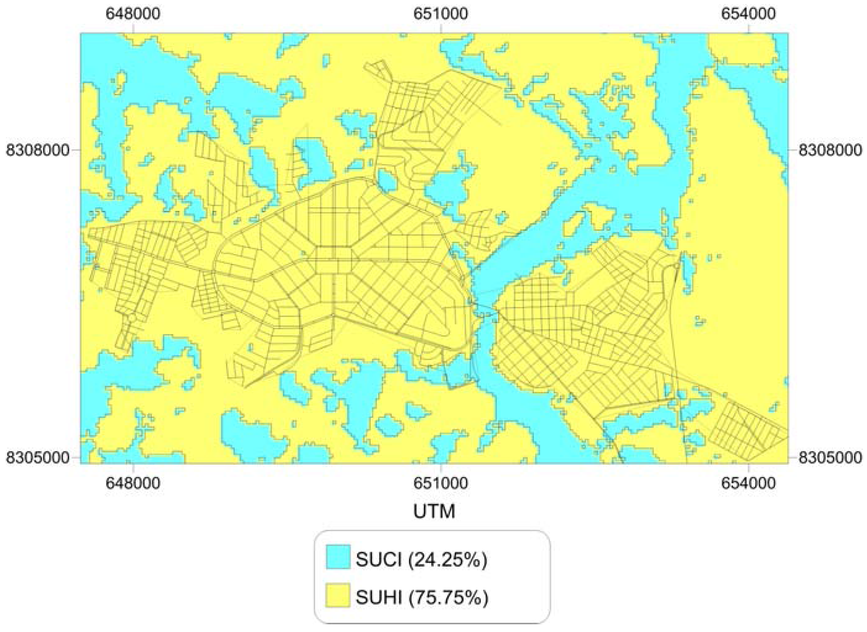
As shown in Figure 7 and

Table 3. Area occupied by the classes of average SUHIs and SUCIs in the Ceres and Rialma cities and surroundings.

SUCI/SUHI (°C)	−6 to −5	−5 to −4	−4 to −3	−3 to −2	−2 to −1	−1 to 0	0 to 1	1 to 2	2 to 3	3 to 4	4 to 5	5 to 6
Area (km2)	0.03	0.33	0.28	0.71	1.84	3.92	5.85	6.37	4.23	2.70	2.16	0.9
Area (%)	0.11	1.14	0.95	2.41	6.26	13.37	19.95	21.75	14.42	9.20	7.38	3.06

, in the study area, there was predominance of SUHIs at the expense of SUCIs. SUHIs occupied an area three times larger than SUCIs; this finding reflects a typically urban problem, the lack of green areas and trees on sidewalks, as it is noted that most of the existing SUCIs are located next to watercourses and steep slopes. SUHIs of 1 °C to 2 °C occurred in most of the study area (21.75% of the total area). The intensity of 5 °C to 6 °C covered a smaller area (0.9 km²), and in the SUCIs with intensity of −6 °C to −5 °C, there was an even smaller area (0.03 km²). The largest area of SUCIs was found from −1 °C to 0 °C (3.93 km²).

3.3. Relationships between LST and $NDVI$

In the summer and spring, periods of high solar radiation and insolation, the highest LST (±40 °C) and $NDVI$ (0.57) values were observed. In Erbil, Iraq, a maximum LST of 53 was observed [27]. The lowest LST values were observed in the autumn (minimum of 18.87 °C), followed by winter. The standard deviations of LST were similar in all seasons; in relation to the $NDVI$, the smallest deviations occurred during autumn and winter, as shown in

Table 4. Seasonal statistics of LST and $NDVI$ in the urban buffer.

Statistics	Spring		Autumn		Summer		Winter
	LST	$\mathit{N}\mathit{D}\mathit{V}\mathit{I}$	LST	$\mathit{N}\mathit{D}\mathit{V}\mathit{I}$	LST	$\mathit{N}\mathit{D}\mathit{V}\mathit{I}$	LST	$\mathit{N}\mathit{D}\mathit{V}\mathit{I}$
Minimum	26.60	−0.16	19.87	−0.08	26.68	−0.20	24.35	−0.13
Average	35.04	0.22	27.88	0.23	35.62	0.23	32.57	0.15
Maximum	40.22	0.56	32.64	0.49	40.70	0.57	38.88	0.45
Standard Deviation	2.10	0.09	2.00	0.07	2.15	0.09	1.99	0.05

.

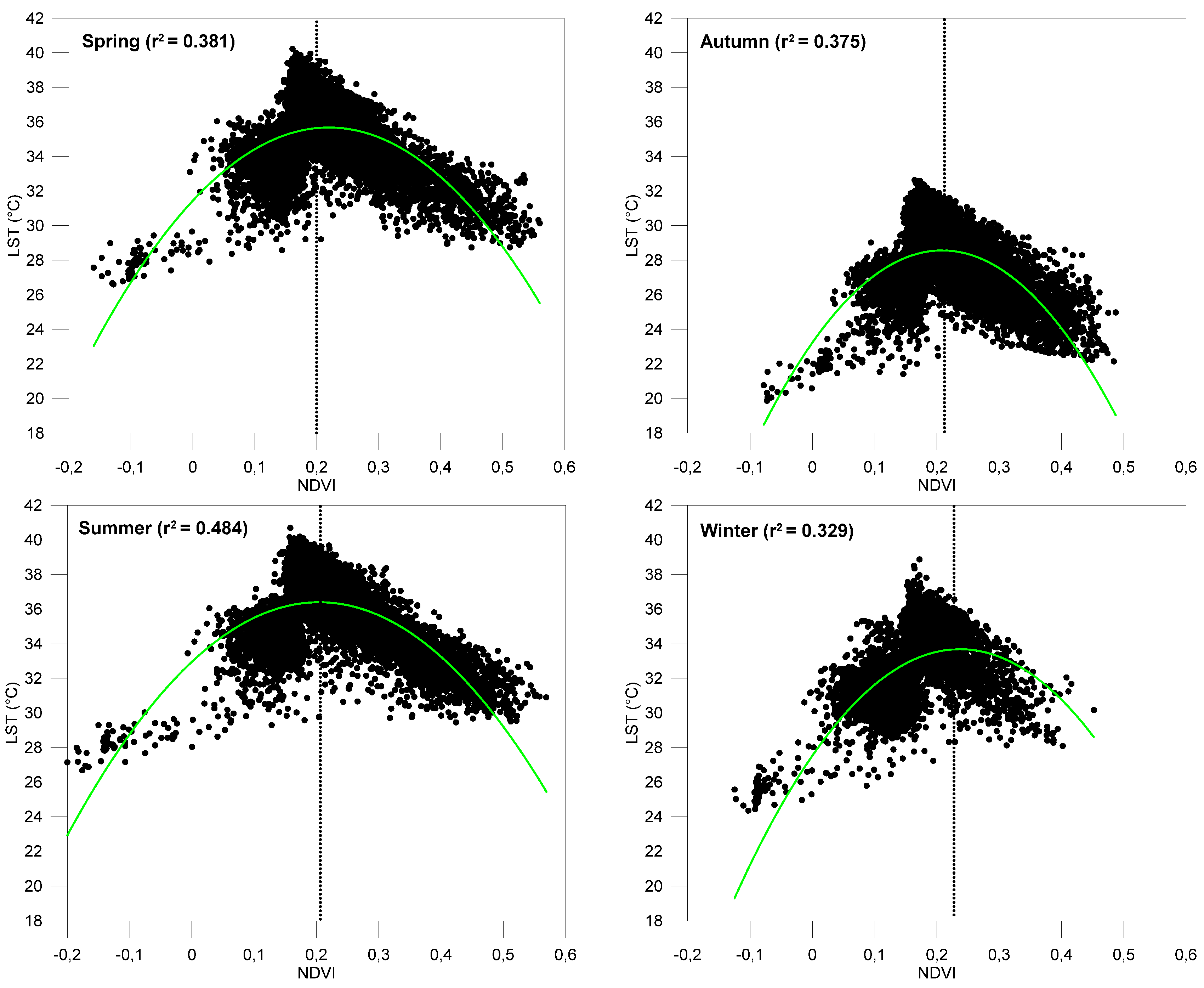
The relationship between LST and $NDVI$ is not always negative [25,27,33] and may vary seasonally, depending on the type of vegetation. In Ceres and Rialma, there is an interesting observation (Figure 8): in all seasons, two relationships were observed, one positive and one negative. An $NDVI$ of 0.2 is the divider of this relationship; up to this point, the relationship is positive, that is, the higher the $NDVI$ value, the higher the surface temperature, while above an $NDVI$ of 0.2, the relationship is negative, i.e., the higher the $NDVI$, the lower the surface temperature. This relationship is interesting because it shows that vegetation with poor physiological conditions cannot minimize the surface temperature in the study area.

4. Conclusions

The surface urban heat island is an important factor in the dynamics of urban climate; its spatial and temporal variation impacts the thermodynamic system of cities.

The different surfaces of the soil absorb and emit radiation at different intensities. Hence, understanding the variation in the intensity of SUHIs can provide subsidies to urban planners and administrators, so that they can reduce the negative effects of urbanization on the climate of cities.

In large cities, the SUHIs are already widely studied, especially at middle and high latitudes. In tropical regions, especially in the small towns of Brazil, little is known about the SUHI phenomenon. The present study provides evidence that the thermal patterns in small towns are different from those in large cities.

In large cities, a more intense SUHI core is evident, because of the spatial configuration of the buildings, especially in the center. In the urban agglomerate of Ceres-Rialma, a SUHI core was not observed. In general, the SUHIs within the urban boundary showed high intensities. The main factor stems from the way in which the soil is covered in small towns, whereas a pattern set by large cities is not observed: the center consists of commercial buildings with a maximum of three floors and households; the area surrounding the center has mainly, households; the peripheral region has spaced homes. This configuration does not allow such a difference as in large cities but creates a relatively homogeneous area of SUHIs.

References

- Morabito, M.; Crisci, A.; Messeri, A.; Orlandini, S.; Raschi, A.; Maracchi, G.; Munafò, M. The impact of built-up surfaces on land surface temperatures in Italian urban areas. Sci. Total Environ. 2016, 551–552, 317–326. [Google Scholar] [CrossRef] [PubMed]
- Arnfield, A.J. Two decades of urban climate research: A review of turbulence, exchanges of energy and water, and the urban heat island. Int. J. Climatol. 2003, 23, 1–26. [Google Scholar] [CrossRef]
- Ngie, A.; Abutaleb, K.; Ahmed, F.; Darwish, A.; Ahmed, M. Assessment of urban heat island using satellite remotely sensed imagery: A review. S. Afr. Geogr. J. 2014, 96, 198–214. [Google Scholar] [CrossRef]
- Stathopoulou, M.; Cartalis, C. Daytime urban heat islands from Landsat ETM+ and Corine land cover data: An application to major cities in Greece. Sol. Energy 2007, 81, 358–368. [Google Scholar] [CrossRef]
- Rasul, A.; Balzter, H.; Smith, C. Spatial variation of the daytime Surface Urban Cool Island during the dry season in Erbil, Iraqi Kurdistan, from Landsat 8. Urban Clim. 2015, 14, 176–186. [Google Scholar] [CrossRef]
- Alcoforado, M.J.; Lopes, A.; Alves, E.D.L.; Canário, P. Lisbon heat island: Statistical study (2004–2012). Finisterra 2014, 49, 61–80. [Google Scholar] [CrossRef]
- Oke, T.R. Boundary Layer Climates, 2nd ed.; Routledge: London, UK, 1987. [Google Scholar]
- Tan, J.; Zheng, Y.; Tang, X.; Guo, C.; Li, L.; Song, G.; Zhen, X.; Yuan, D.; Kalkstein, A.J.; Li, F.; et al. The urban heat island and its impact on heat waves and human health in Shanghai. Int. J. Biometeorol. 2010, 54, 75–84. [Google Scholar] [CrossRef] [PubMed]
- Rosenfeld, A.H.; Akbari, H.; Romm, J.J.; Pomerantz, M. Cool communities: Strategies for heat island mitigation and smog reduction. Energy Build. 1998, 28, 51–62. [Google Scholar] [CrossRef]
- Agarwal, M.; Tandon, A. Modeling of the urban heat island in the form of mesoscale wind and of its effect on air pollution dispersal. Appl. Math. Model. 2010, 34, 2520–2530. [Google Scholar] [CrossRef]
- Magli, S.; Lodi, C.; Lombroso, L.; Muscio, A.; Teggi, S. Analysis of the urban heat island effects on building energy consumption. Int. J. Energy Environ. Eng. 2015, 6, 91–99. [Google Scholar] [CrossRef]
- Weng, Q.; Yang, S. Managing the adverse thermal effects of urban development in a densely populated Chinese city. J. Environ. Manag. 2004, 70, 145–156. [Google Scholar] [CrossRef]
- Guhathakurta, S.; Gober, P. The impact of the phoenix urban heat island on residential water use. J. Am. Plan. Assoc. 2007, 73, 317–329. [Google Scholar] [CrossRef]
- IBGE. Cidades. 2015. Available online: http://www.cidades.ibge.gov.br/ (accessed on 1 September 2016). [Google Scholar]
- Isaya Ndossi, M.; Avdan, U. Application of open source coding technologies in the production of Land Surface Temperature (LST) maps from Landsat: A PyQGIS plugin. Remote Sens. 2016, 8, 413. [Google Scholar] [CrossRef]
- Zhang, X.; Zhong, T.; Feng, X.; Wang, K. Estimation of the relationship between vegetation patches and urban land surface temperature with remote sensing. Int. J. Remote Sens. 2009, 30, 2105–2118. [Google Scholar] [CrossRef]
- USGS. Earth Explorer. 2016. Available online: http://earthexplorer.usgs.gov/ (accessed on 1 August 2016). [Google Scholar]
- USGS. Using the USGS Landsat 8 Product. 2016. Available online: http://landsat.usgs.gov/Landsat8_Using_ (accessed on 1 August 2016). [Google Scholar]
- Zhang, J.; Wang, Y.; Li, Y. A C++ program for retrieving land surface temperature from the data of Landsat TM/ETM+ band6. Comput. Geosci. 2006, 32, 1796–1805. [Google Scholar] [CrossRef]
- Artis, D.A.; Carnahan, W.H. Survey of emissivity variability in thermography of urban areas. Remote Sens. Environ. 1982, 12, 313–329. [Google Scholar] [CrossRef]
- Sinha, S.; Pandey, P.C.; Sharma, L.K.; Nathawat, M.S.; Kumar, P.; Kanga, S. Remote Estimation of Land Surface Temperature for Different LULC Features of A Moist Deciduous Tropical Forest Region; Springer International Publishing: Berlin, Germany, 2014. [Google Scholar]
- Cao, X.; Onishi, A.; Chen, J.; Imura, H. Quantifying the cool island intensity of urban parks using ASTER and IKONOS data. Landsc. Urban Plan. 2010, 96, 224–231. [Google Scholar] [CrossRef]
- Lopes, A.; Alves, E.; Alcoforado, M.J.; Machete, R. Lisbon urban heat island updated: New highlights about the relationships between thermal patterns and wind regimes. Adv. Meteorol. 2013, 2013, 1–11. [Google Scholar] [CrossRef]
- Li, S.; Mo, H.; Dai, Y. Spatio-temporal pattern of urban cool island intensity and its eco-environmental response in chang-zhu-tan urban agglomeration. Commun. Inf. Sci. Manag. Eng. 2011, 1, 1–6. [Google Scholar]
- Haashemi, S.; Weng, Q.; Darvishi, A.; Alavipanah, S. Seasonal variations of the surface urban heat island in a semi-arid city. Remote Sens. 2016, 8, 352. [Google Scholar] [CrossRef]
- Gémes, O.; Tobak, Z.; van Leeuwen, B. Satellite based analysis of surface urban heat island intensity. J. Environ. Geogr. 2016, 9, 23–30. [Google Scholar] [CrossRef]
- Rasul, A.; Balzter, H.; Smith, C. Diurnal and seasonal variation of surface urban cool and heat islands in the semi-arid city of Erbil, Iraq. Climate 2016, 4, 42. [Google Scholar] [CrossRef]
- Becerra, J.A.B.; Shimabukuro, Y.E.; dos Santos Alvalá, R.C. Relação do padrão sazonal da vegetação com a precipitação na região de cerrado da Amazônia Legal, usando índices espectrais de vegetação. Rev. Bras. Meteorol. 2009, 24, 125–134. [Google Scholar] [CrossRef]
- Nichol, J.E.; To, P.H. Temporal characteristics of thermal satellite images for urban heat stress and heat island mapping. ISPRS J. Photogramm. Remote Sens. 2012, 74, 153–162. [Google Scholar] [CrossRef]
- Schwarz, N.; Manceur, A.M. Analyzing the influence of urban forms on surface urban heat islands in Europe. J. Urban Plan. Dev. 2015, 141, A4014003. [Google Scholar] [CrossRef]
- Benas, N.; Chrysoulakis, N.; Cartalis, C. Trends of urban surface temperature and heat island characteristics in the Mediterranean. Theor. Appl. Climatol. 2016. [Google Scholar] [CrossRef]
- Sobrino, J.A.; Jiménez-Muñoz, J.C.; Paolini, L. Land surface temperature retrieval from LANDSAT TM 5. Remote Sens. Environ. 2004, 90, 434–440. [Google Scholar] [CrossRef]
- Sun, D.; Kafatos, M. Note on the NDVI-LST relationship and the use of temperature-related drought indices over North America. Geophys. Res. Lett. 2007, 34, L24406. [Google Scholar] [CrossRef]
© 2016 by the author; licensee MDPI, Basel, Switzerland. This article is an open access article distributed under the terms and conditions of the Creative Commons Attribution (CC-BY) license (http://creativecommons.org/licenses/by/4.0/).