Land Surface Temperature Variation Due to Changes in Elevation in Northwest Vietnam


1
Cartography, GIS and Remote Sensing Department, Institute of Geography, University of Göttingen, Goldschmidt Street 5, Göttingen 37077, Germany
2
Cartography and Geodesy Department, Land Management Faculty, Vietnam National University of Agriculture, Hanoi 100000, Vietnam
*
Author to whom correspondence should be addressed.
Climate 2018, 6(2), 28; https://doi.org/10.3390/cli6020028
Submission received: 25 January 2018
/
Revised: 6 April 2018
/
Accepted: 7 April 2018
/
Published: 13 April 2018
Abstract
:Land surface temperature (LST) is one of the most important variables for applications relating to the physics of land surface processes. LST rapidly changes in both space and time, and knowledge of LST and its spatiotemporal variation is essential to understand the interactions between human activity and the environment. This study investigates the spatiotemporal variation of LST according to changes in elevation. The newest version (version 6) of MODIS LST data for 2015 was used. An area of 40,000 km2 (200 × 200 km2) in northwest Vietnam with elevations ranging from 8 m to 3165 m was chosen as a case study. Our results showed that the drop in LST with increased elevation varied throughout the year during both the daytime and nighttime. The monthly averages in 2015 and an altitude increase of 1000 m resulted in a decrease in LST ranging from 3.8 °C to 6.1 °C and 1.5 °C to 5.8 °C for the daytime and nighttime, respectively. This suggests that in any study relating to the spatial distribution of LST, the effect of elevation on LST should be considered. In addition, the effects of land use/cover and elevation distribution on the relationship between LST and elevation are discussed.
1. Introduction
Land surface temperature (LST), defined as the “skin” temperature of the earth surface, is a key parameter for land-surface processing studies at both a regional and global scale [1,2,3,4]. Knowledge of LST and its spatiotemporal variation within regions is of fundamental importance to understanding the interactions between human activity (e.g., change in land use) and the environment [5]. As the LST varies both spatially and temporally, ground-based station observations cannot represent the LST of a region, particularly in developing countries where weather stations are very sparse. Currently, remote sensing satellite data is the most suitable way to study LST spatial and temporal variations [6,7,8]. The most popular remote sensing images used to retrieve LST are moderate resolution imaging spectroradiometer (MODIS), advanced very high resolution radiometer (AVHRR), enhanced thematic mapper plus (ETM+), and the advanced spaceborne thermal emission and reflection radiometer (ASTER). Due to the high temporal resolutions (four times per day) of MODIS LST, its data is widely applied in remote sensing communities.
MODIS LST data has been available since early 2000 and mid-2002 from Terra and Aqua satellites, respectively. There are seven MODIS LST products with temporal resolutions of daily (MOD/MYD11A1, MOD/MYD11B1, MOD/MYD11C1, and MOD/MYD11_L2), eight-day (MOD/MYD11A2, MOD/MYD11C2), and monthly (MOD/MYD11C3) data. Each product consists of daytime and nighttime LST. Thus, by using both the Terra and Aqua daily products, the highest temporal resolution (i.e., four times per day) can be achieved. In August 2015, version 6 (V6) of MODIS LST was released and free to download [9]. Wan [10] studied and evaluated MODIS LST version 6 (using Aqua MODIS daily swath data). The results showed that the accuracy was superior to the previous versions (i.e., V4.1 and V5).
Since available, MODIS LST data has been used for various studies, such as evaluating and monitoring urban heat islands [11,12,13,14,15], estimating air surface temperatures (Ta) [16,17,18,19], retrieving soil moisture [20,21], drought assessment [22], and hydrology applications [23]. Most of these studies have shown that the changes of land surface properties (e.g., normalized difference vegetation index (NDVI), elevation, and land use/cover types) will result in the variations of LST [3]. Among these, the relationship between LST and NDVI or the effects of land use/cover on LST have been widely studied [13,24,25]. A few studies have investigated the direct effect of elevation on LST; however, elevation was found to have an impact on most studies using MODIS LST, particularly those conducted over a large area where the terrain is variable. For example, in Ta estimation using MODIS LST data, along with LST, elevation was considered one of the most impactful variables effecting the results of Ta estimation [14,26,27].
It is known that for a stationary atmosphere, an increase in elevation leads to a subsequent decrease in air pressure and Ta. This decrease is referred to as the environmental lapse rate and occurs at any location along the vertical direction [3]. For every 1000 m increase, the environmental lapse rate varies between 5 °C to 10 °C, depending on the moisture condition [3]. According to Kenawy et al. [28], different regions show a different variability of Ta, as each region has a unique terrain [29,30,31]. Moreover, the variation of Ta was not consistent between high and low land areas. Beniston [32] found that Ta increased more rapidly at higher than at lower elevations. Being consistent with Beniston [32], some high mountainous areas in the Tibetan Plateau showed a more rapid change in temperature than in lower regions [33]. Various studies have investigated the relationship between Ta and elevation. The majority of these studies used point data from weather stations located 1.5 m to 2.0 m above the land surface [33,34,35]. LST and Ta are not equivalent, and their relationship is multifaceted due to the complex surface energy budget and the multiple related variables between them [17,18,19,36]. Therefore, the relationship between Ta and elevation is different from those of LST and elevation. As mentioned above, the effect of land surface characteristics (e.g., NDVI and soil moisture) on LST has been studied [3]; meanwhile, the effects of elevation on LST are rarely documented. To the best of our knowledge, few studies have investigated the direct relationship between LST and elevation using remote sensing LST data. Recently, Khandelwal et al. [3] assessed the variation of LST with changes of elevation in Jaipur, India. However, the study used only nighttime MODIS Aqua LST for three seasons with a narrow elevation range (215 m to 530 m). Furthermore, no studies from Vietnam have investigated the relationship between LST and elevation using remote sensing image data, particularly MODIS LST data. It is therefore necessary to assess the spatiotemporal variations of LST with changes of elevation in northern Vietnam using the MODIS LST V6 data.
The main objectives of this study were to: (i) evaluate and assess the relationship between monthly LST and elevation for 2015 in northern Vietnam, and (ii) discuss the effects of land use/cover, elevation distribution, and latitude and longitude on the relationship between LST and elevation.
2. Materials and Methods
2.1. Study Area
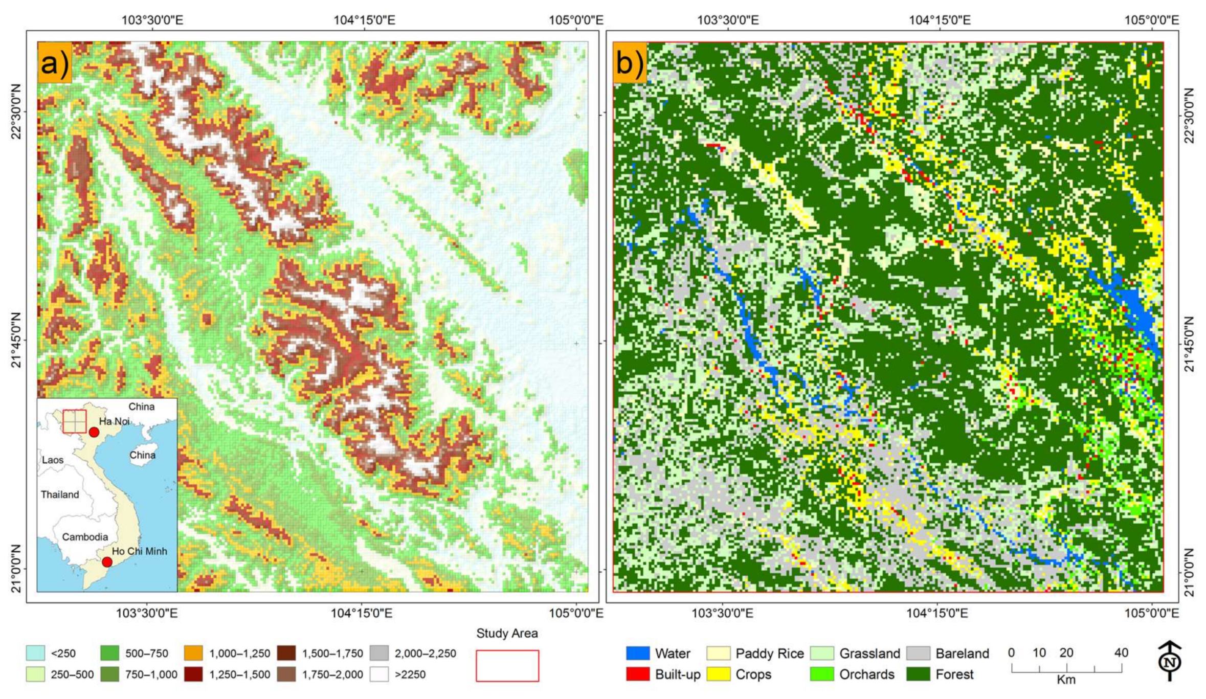
The study was conducted in a 40,000 km2 (200 × 200 km2) area in northwest Vietnam (Figure 1). The elevation ranges from 8 m to 3165 m with the majority of areas below 1000 m and a mean elevation of 800 metres above sea level (m a.s.l). The northwest regions of Vietnam were selected to reduce the influence of the urban heat island (UHI) effect due to the impact of the capital, Hanoi, on the results. Uniform study areas of 200 × 200 km2 were chosen to balance the effects of longitude and latitude.
2.2. Data
2.2.1. MODIS LST
MODIS aboard Terra and Aqua satellites provide daily, eight-day, and monthly LST data at resolutions of typically 1 km and 6 km. Wan [10] studied and evaluated LST V6 data using Aqua MODIS and stated that the accuracy was better than for previous versions (i.e., V4.1 and V5) due to fixes and improvements. The most important improvements were removing cloud-contaminated LST pixels from MODIS level 2 and 3 products and updating split-window algorithm coefficients [10]. In this study, we assessed the variation of LST due to changes in elevation using eight-day LST data (daytime and nighttime) from the Aqua satellite MYD11A2. The eight-day MYD11A2 data were achieved by averaging all valid daily LST data under clear sky conditions. The number of daily LST data involved in calculating the eight-day LST data vary from two to eight, depending on data availability [10]. There are 12 science data set (SDS) layers within MYD11A2 data, including LST, quality control, view time, view angle, clear sky conditions for day and night, and emissivity bands 31 and 32. For this study, 46 MODIS images (h27v06, V6, 2015) of MYD11A2 product in hierarchical data format (HDF) were downloaded from the Land Processes Distributed Active Archive Center (LP DAAC) [9].
2.2.2. Elevation
The elevation across the study area ranged from 8 m to over 3165 m (Figure 1). Elevation data with a spatial resolution of approximately 30 m (1 arc) was retrieved from the U.S. Geological Survey (USGS) ASTER global DEM. To align the elevation data with LST data, it was resampled to a resolution of 1000 m using the nearest neighbor sampling approach in ArcMap 10.5 software.
2.2.3. Land Cover
Land use and land cover data were downloaded from the Japanese Aerospace Exploration Agency (JAXA) [37]. Data was available for spatial resolutions of 15 m and 250 m for 2007 and 2015. The 2015 land use/cover map had a high overall accuracy (89.1%) with a κ coefficient of 0.872. It included nine different land use/cover classes, with the following eight classes found within the study area: water, urban and built-up, rice paddy, crops, grassland, orchards, bare land, and forest (Figure 1b). To be consistent with other data, the map was resampled to 1000 m using the nearest neighbor sampling approach in ArcMap 10.5 software.
2.3. Preprocessing and Data Analysis
The MYD11A2 data was downloaded from the LP DAAC website in HDF format using the sinusoidal projection system [9]. MODIS reprojection tools provided by LP DAAC were used to reproject MYD11A2 product to the UTM Zone 48 N projection system with WGS84 datum. Among the 12 science data set layers of MYD11A2, LST (day and night) and the quality control (QC) layer were selected and reformatted to GeoTIFF for further analysis. ArcMap 10.5 was used to analyze the data in GeoTIFF format.
MODIS LST and QC data in GeoTIFF with a resolution of 926.65 m were resampled to 1000 m using the nearest neighbor resampling approach. The images were then clipped to the study area extent using ArcMap 10.5 software.
Cloudy pixels from MODIS LST were removed by the generalized split-window algorithm [38]; however, there were still pixels associated with thin clouds which the algorithm was unable to detect and remove. The quality information (QC file) of each image was therefore used for removing such data, and only LST data with an average error below or equal to 2 K were used for further analysis.
All valid LST pixels (in digital number—DN value) were converted to Celsius (°C) using the following equation:
where °C is the temperature in Celsius and 0.02 is the scale factor of the MODIS LST product [9].
LST (°C) = 0.02 × DN − 273.15
2.4. Relationship between LST and Elevation
The spatial and temporal relationship between monthly average LST (°C) and elevation (m) were investigated. Based on the Julian calendar of 2015, we divided the 46 eight-day LST images into 12 months. We then applied the same rule of calculating an eight-day LST from a daily LST for calculating the average monthly LST; that is, the monthly LST data was averaged from one to four eight-day LST data. Linear regression models were used to evaluate the relationship between LST and elevation.
3. Results
3.1. Spatiotemporal Variation of LST
Figure 2 shows the nighttime and daytime LST average from January to December in 2015 in northwest Vietnam. In general, the LST ranged from 11 °C to 25 °C during the nighttime and 21 °C to 35 °C during the daytime. It should be noted that, because LST data are not available for a location (pixel) covered by cloud, therefore, there are some blank pixels (white color) in the daytime and nighttime (e.g., in June). For all months, the LST for the highest topographic area—from the northwest to the southeast region—was lower than other areas in the study site. This was clearly seen for both the daytime and nighttime. The lowest elevation area (northeast) always showed the highest nighttime LST. However, the highest daytime LST were observed in the south-center region from March to June. This indicates that not only elevation influences LST, but also other factors, such as land use/cover. As shown in Figure 1, this area is mainly covered by bare land and crops; however, crop planting started between April and May, and therefore in the period from March to June, the main land cover was bare land. This is consistent with the study of Xu et al. [39], which was implemented in the Tibetan Plateau from 2003 to 2010. In this study, Xu et al. [39] concluded that bare land has the highest mean LST in comparison to four others land cover types: forest, grassland, water, and snow/ice. The daytime and nighttime differences indicate that the topography had a higher influence on the nighttime LST than the daytime LST.
In addition, the different LST between high and low elevations varied across different months and different times of the day. Figure 2 shows that while the difference in LST between high and low elevation was not clear for the daytime from June to October, there was a clear difference at nighttime.
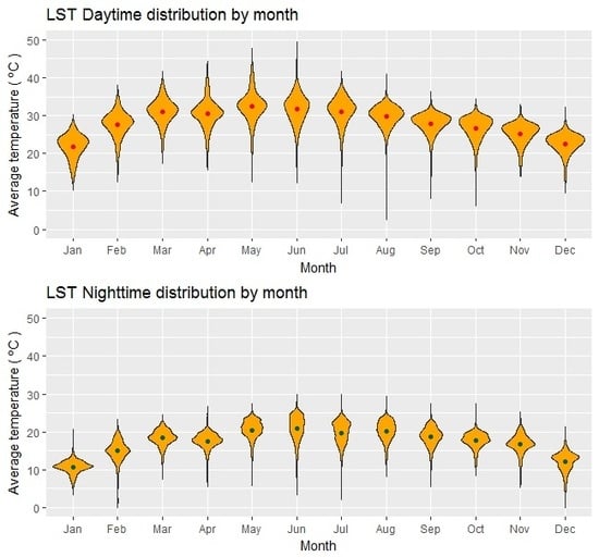
Figure 3 shows the temporal variation of monthly LST from January to December in 2015, in which the daytime LST was larger than that of the nighttime. This is consistent with the results shown in Figure 2. It should be mentioned that the average monthly LST were calculated from 40,000-pixel values (200 × 200) containing different land covers and elevations. Therefore, the values of LST varied in all months and regions (Figure 2 and Figure 3). LST increased from January to April, reached the highest in June, and decreased thereafter. June was the hottest month during both the daytime and nighttime, whereas January and December had the lowest daytime and nighttime LST.
3.2. LST and Elevation
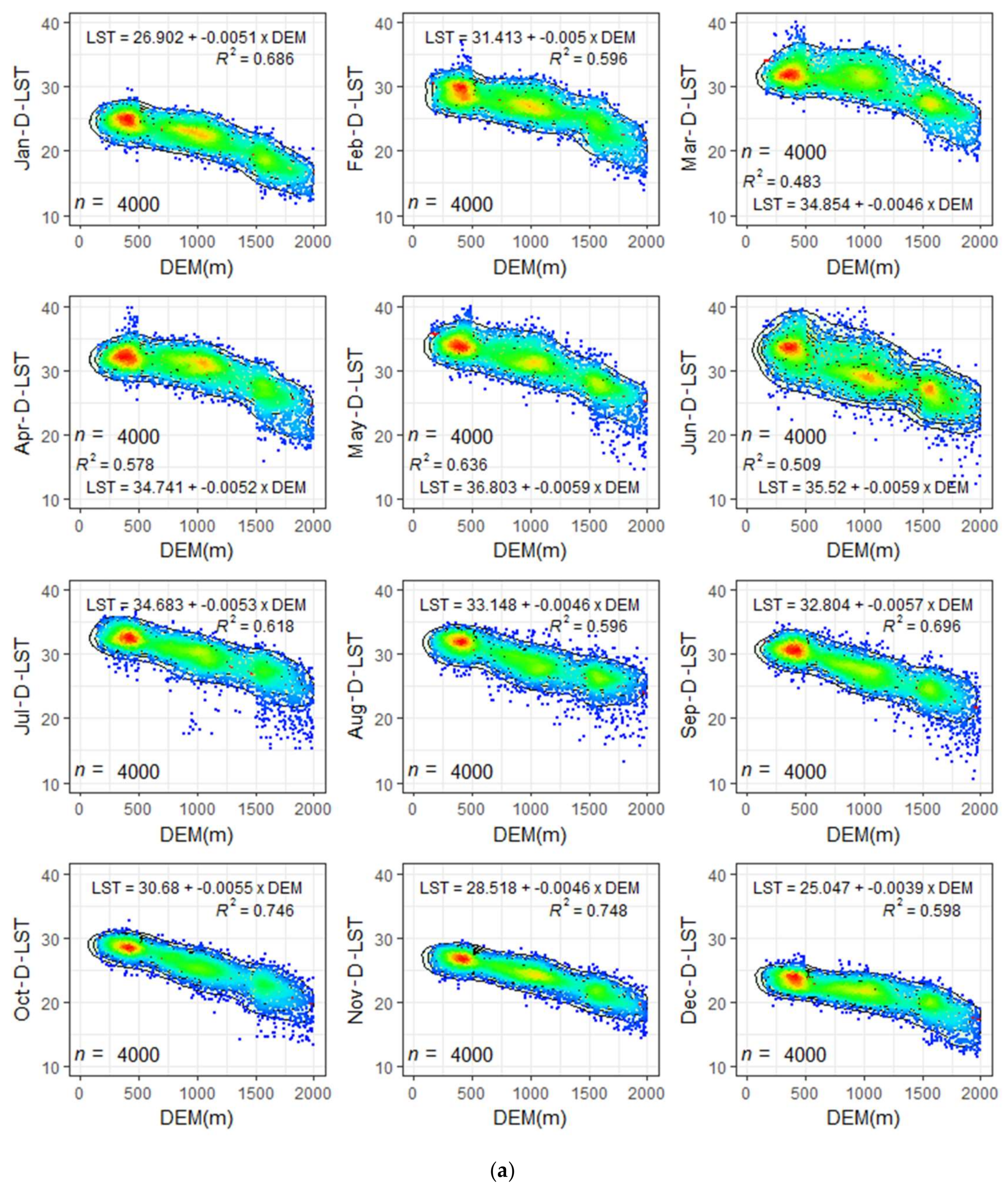
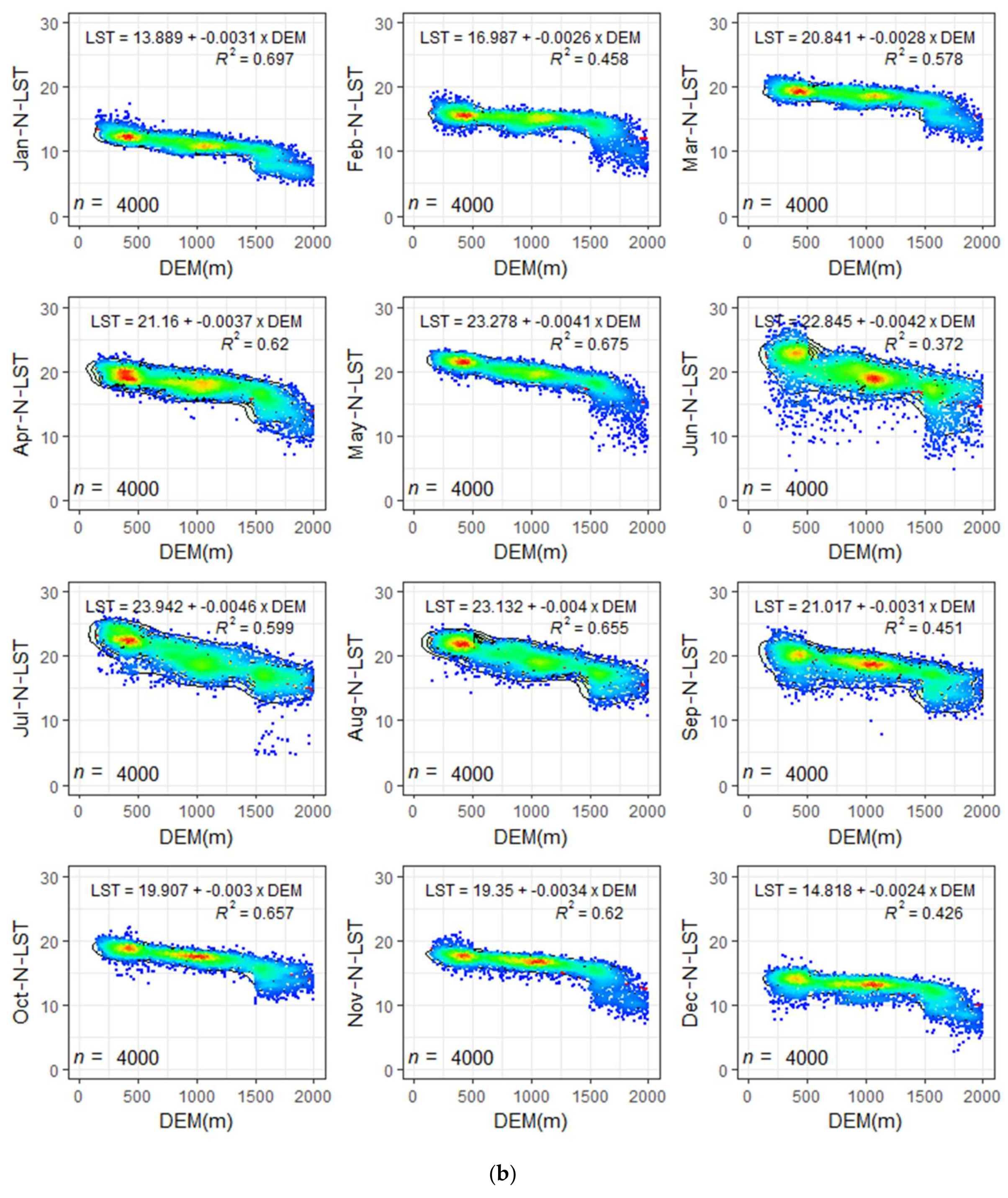
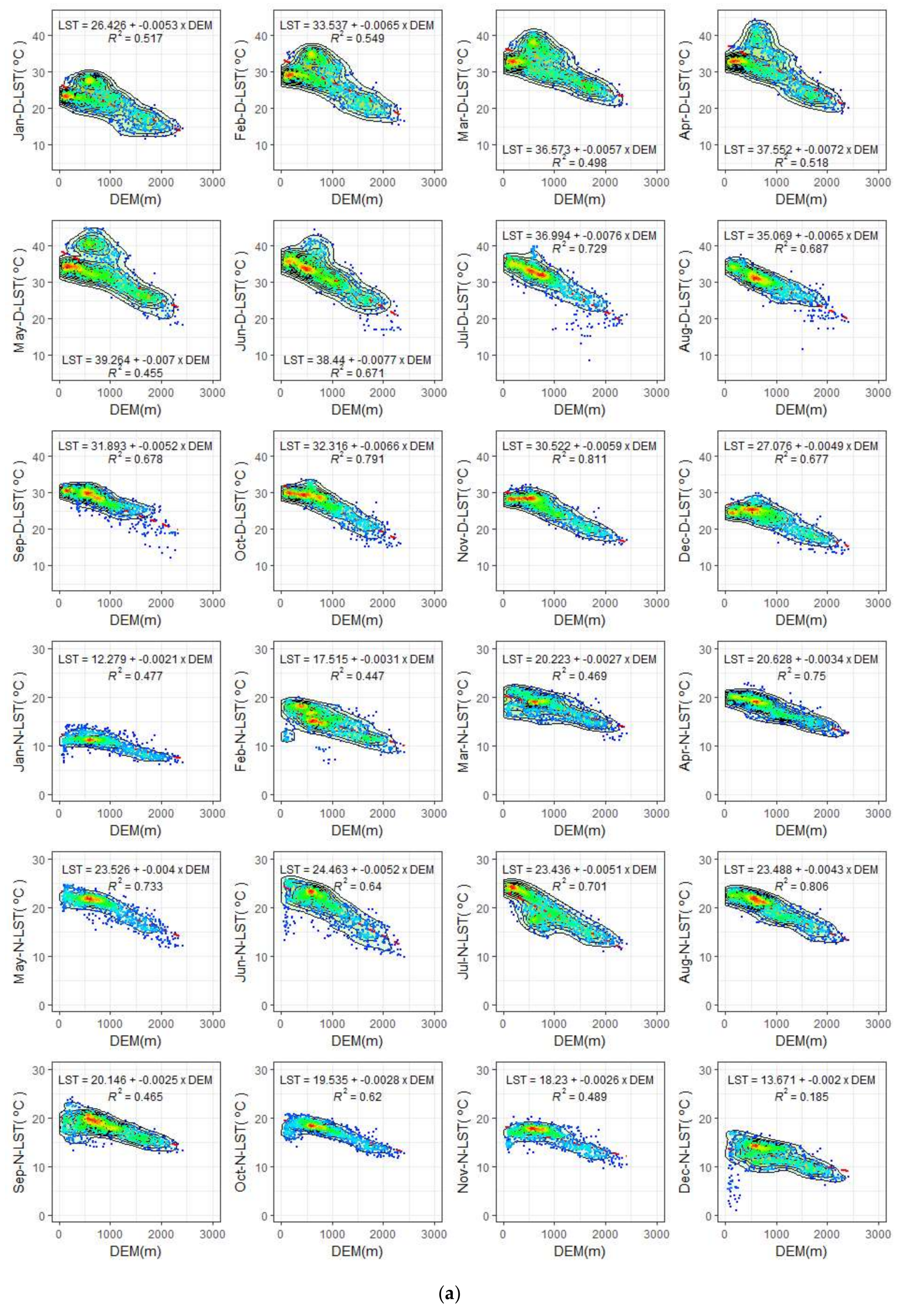
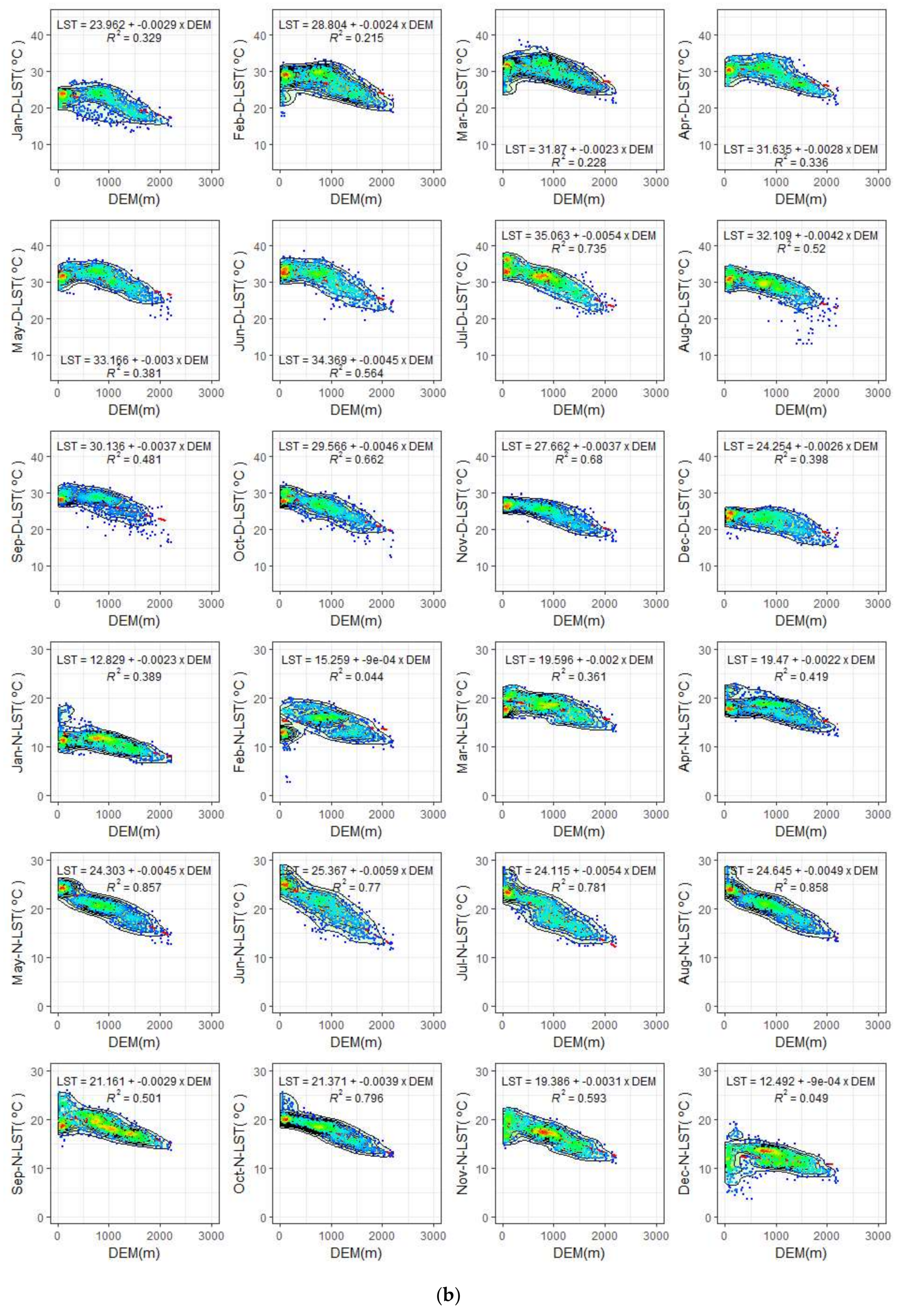
Figure 4 shows the linear regression models between averaged monthly daytime (Figure 4a) and nighttime (Figure 4b) LST and elevations in northwest Vietnam. The negative correlation confirms the well-known relationship between temperature and topography [40]. As shown in Figure 4a,b, the correlation between LST and elevation was stronger at nighttime than daytime, except for four months: February, September, November, and December. This may reflect that several pixels within low regions (0 m to 1000 m) had a very low LST, ranging from 0 °C to 10 °C in December and February and 10 °C to 15 °C in September and November.
The relationship between LST and elevation not only varied between months, but also between the daytime and nighttime. Figure 4a,b shows that there were stronger correlations in hotter months (May to August) during the nighttime, whereas a weaker correlation for the hotter months was seen for the daytime. The highest correlations were observed in October (R2 = 0.701) and in August (R2 = 0.809) at daytime and nighttime, respectively.
Figure 4a shows that during the day, the linear regression slope ranges from −0.0038 to −0.0061. This indicates that for each 1000 m elevation increase, the LST decreases from 3.8 °C to 6.1 °C. Based on the R2 value and the slope, the smallest and largest changes of LST corresponding to the elevation are in January and July, respectively.
The intercept varies from 24.77 to 36.18 (daytime) and 12.62 to 25.26 (nighttime) each month and is slightly higher than the average monthly LST (Figure 3) of the respective month. This was consistent across all months in 2015 for the daytime and nighttime, indicating a good relationship between intercept value and average LST value.
For the nighttime (Figure 4b), the linear regression slope varied from −0.0015 to −0.0058; that is, for each 1000 m elevation increase, the LST decreased from 1.5 °C to 5.8 °C. The lowest and highest slopes were with LST in December and June, respectively. A strong correlation (R2 of 0.711 to 0.809) between LST and elevation was observed in May, June, July, August, and October. The correlation in January, March, September, and November ranged from 0.465 to 0.588. However, in February and December, these correlations were very low, with an R2 of 0.093 and 0.249 for December and February, respectively. Figure 4b highlights the many low LST points in February and December, suggesting another local factor may have strongly reduced LST.
Except for the trends in February and December, LST at nighttime was generally more closely distributed along the regression line than that of the daytime LST. This may indicate that solar radiation affects the LST during the daytime.
4. Discussion
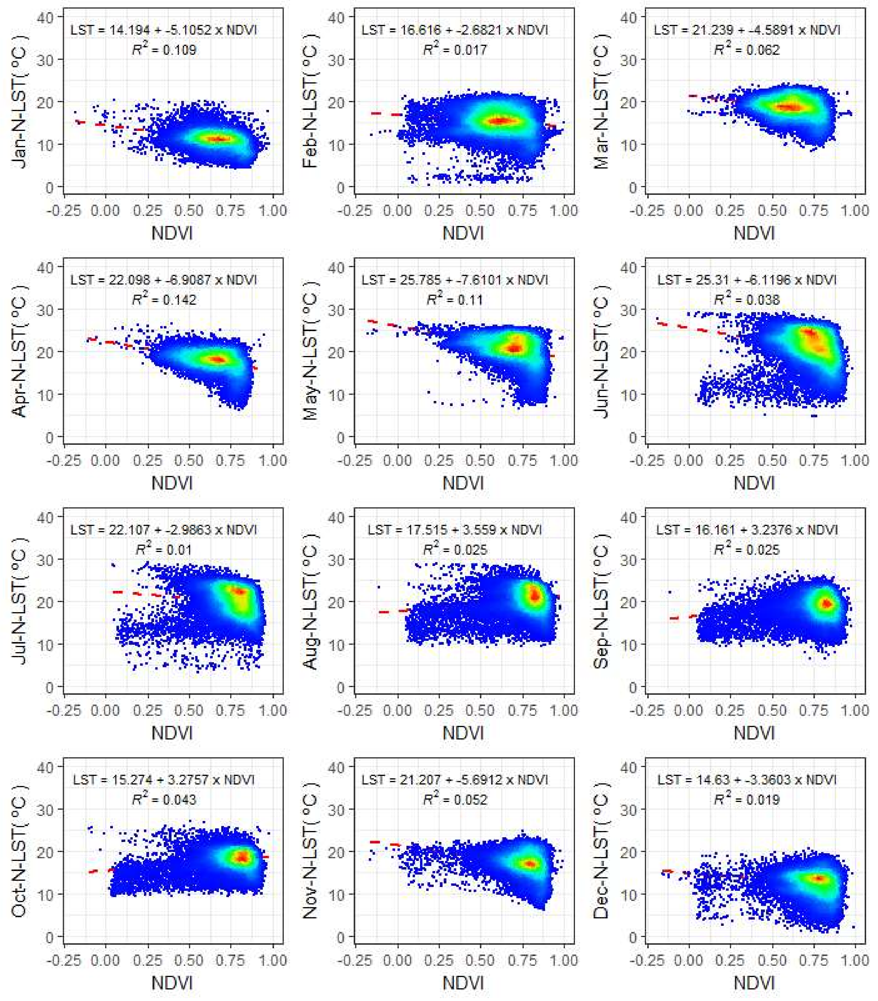
Although this study focuses on the effects of elevation on LST due to its infrequent documentation in literature, an analysis on the relationship between LST and the most popular vegetation index (normalized difference vegetation index, NDVI) was additionally discussed. The relationship between LST and NDVI is shown in Figure A3 and Figure A4 (Appendix C).
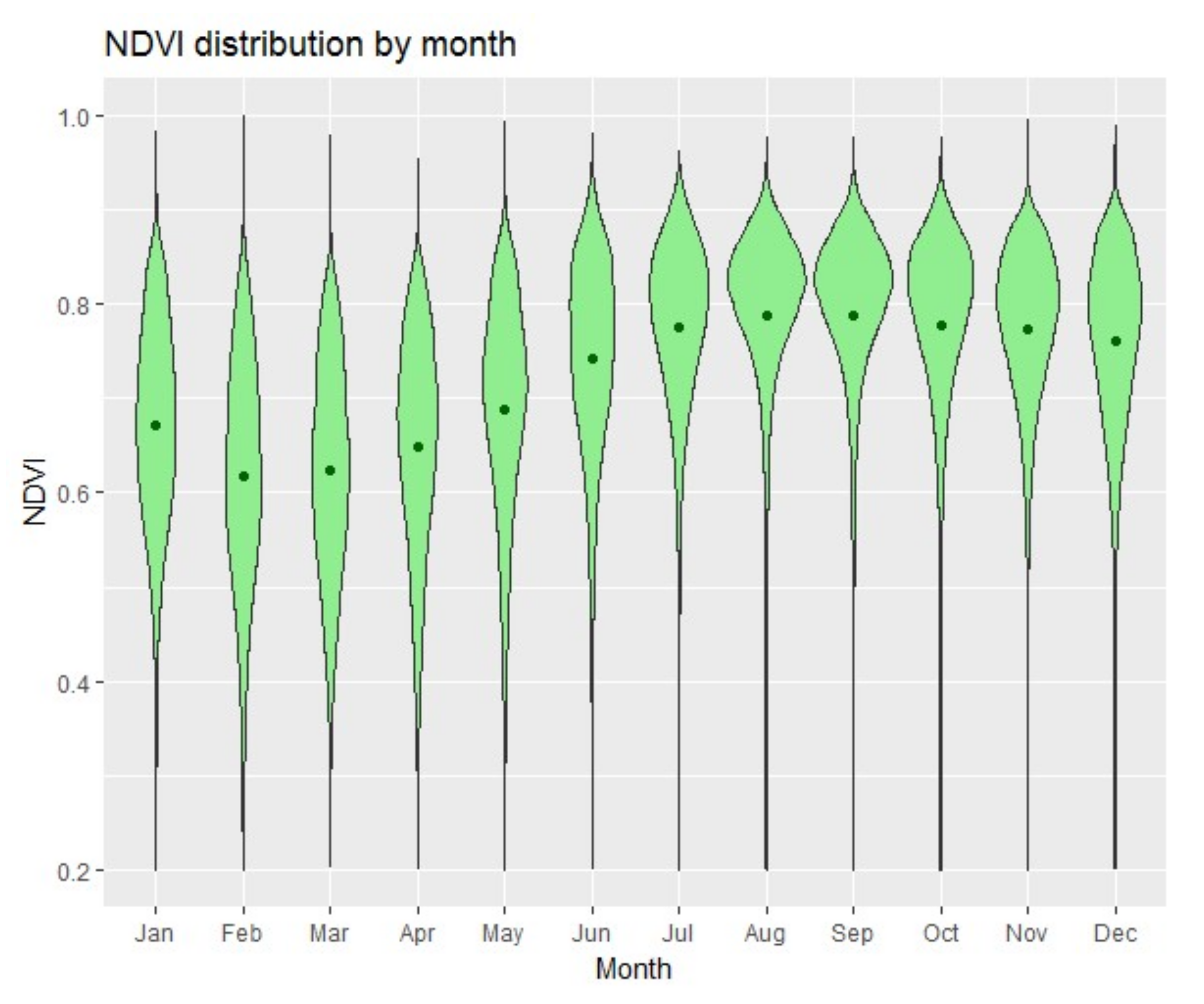
Figure A2 shows the monthly distribution of NDVI in 2015 for the study area. As shown in Figure 1, the major land cover of the study area was forest (51.7%); consequently, the NDVI was quite high, ranging from approximately 0.4 to 0.9 with a monthly average from 0.6 to 0.8 (Figure A2).
The correlation between LST and NDVI (Figure A3 and Figure A4) showed similar results with previous studies; on average LST and NDVI displayed a negative correlation, and the coefficient of determination (R2) of the daytime was slightly higher than those of the nighttime.
In the literature, various studies have shown that land use/cover has a strong impact on LST [41,42,43] and Ta [44,45]. Therefore, in this section, we presented further detail on the relationship between LST and elevation in northwest Vietnam and other potential factors that could have an effect on this relationship, such as land cover and elevation distribution.
4.1. The Influence of Land Use/Cover
In order to assess the effects of land use/cover on the variation of LST according to elevation, we used the high-resolution land use and land cover map products over northern Vietnam in 2015, obtained from the Japanese Aerospace Exploration Agency.
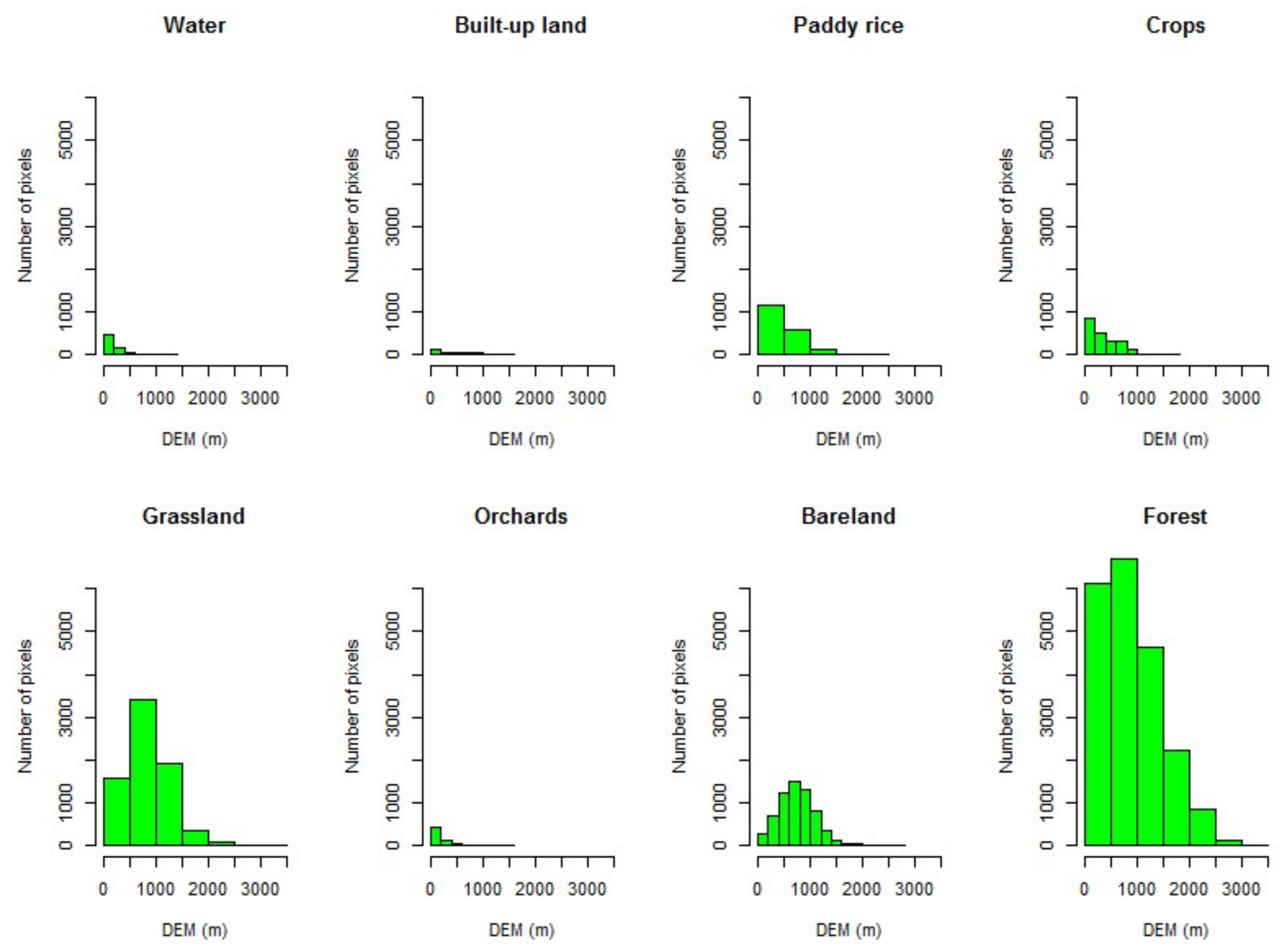
As shown in Figure 5a,b, there were four main land cover types (water, built-up, crops, and orchards) from 8 m to approximately 1000 m. Paddies, grassland, and bare land had a wider elevation range (2000 m to 2200 m). Forests showed the widest elevation range, from 8 m to approximately 3000 m. Figure 5 also shows that the number of pixels for each land cover type were different, ranging from 264 pixels to 20,671 pixels. The major distribution of land use/cover across the study area was forest, grassland, and bare land, which accounted for 51.7%, 18.4%, and 16.0%, respectively (Figure 5). The remaining five land use/cover types only accounted for 13.9% of the total area. The linear regression results of the major land use/cover types were more consistent with the results shown in Section 3 than for the other five land use/cover types. This indicates that the distribution of land use/cover type had an impact on the relationship between LST and elevation in the area.
Another important point is that the change of LST and elevation of each land cover type was significantly different between the daytime and nighttime. Here, we focused on the three major land cover types (grassland, bare land, and forest); the proportion of the other land cover types was low with poorly distributed elevations. As shown in Figure 5a, when the elevation increased by 1000 m, the LST of grassland, bare land, and forest decreased from 4.2 °C, 4.7 °C, and 5.1 °C, respectively, at daytime. However, at nighttime (Figure 5b), these changes were much lower: 3.1 °C, 3.2 °C, and 3.6 °C, respectively.
4.2. The Influence of Topographic Distribution
Figure 4a,b shows that the majority of observations were located at lower elevations (8 m to 1000 m) and that the spatial distribution was imbalanced across the elevations. Figure A1 (Appendix A) shows the number of pixels for the elevation intervals. It is clearly seen that the number of observations at an elevation from 2000 m to 3000 m was much lower than the number of observations at an elevation from 8 m to 2000 m. Therefore, to assess the influence of elevation distribution, all pixels with an elevation over 2000 m were removed. As shown in Figure A1, the number of pixels distributed from 8 m to 2000 m were imbalanced. Therefore, to assess the influences of LST and elevation, a balanced number of observations at four elevation intervals were used: below 500 m (Level 1), 500 m–1000 m (Level 2), 1000 m–1500 m (Level 3), and 1500 m–2000 m (Level 4). For each elevation interval, 1000 pixels were randomly chosen for analysis.
Figure 6a,b shows that the relationship between LST and elevation was much stronger (R2 ranges from 0.372 to 0.748) for all months at both daytime and nighttime than the results of all data shown in Figure 4a,b. The LST dropped from 3.9 °C to 5.9 °C (at daytime) and 2.4 °C to 4.6 °C (at nighttime) for every 1000-m elevation increase.
In this study, the relationship between LST and elevation and changes of longitude and latitude were additionally assessed. Two straight lanes were chosen for evaluation: Lane 1 (north to south) and Lane 2 (west to east). To reduce the effects of latitude and longitude, a line of 5 km width was used. Figure 7a,b shows that the elevations of the two lanes were consistent and ranged from 0 m to approximately 2000 m. During the daytime, LST decreased from 4.9 °C to 7.7 °C as elevation increased by 1000 m (Figure 7a). At nighttime, however, the LST dropped from 2.0 °C to 5.2 °C. Lane 2 (Figure 7b) shows the relationship between LST and elevation, where the longitude was assumed to be stable and the latitude changed by approximately 2° (200 km). During the daytime, the correlation between LST and elevation was much lower than those of Lane 1 (Figure 7a). At nighttime, however, this correlation was high, except in February and December. The shift in LST due to a 1000 m change of elevation was also lower than Lane 1, ranging from 2.3 °C to 5.4 °C and 0 °C to 5.9 °C at daytime and nighttime, respectively. However, it should be noted that in Figure 7b, there were several observations in February and December at low elevations with very low LST in comparison to other months. This may result from unique weather events during these months. To assess the relationship between LST and elevation, such weather events should be considered.
5. Conclusions
In this study, we investigated the influence of elevation on LST of the daytime and nighttime from MODIS LST version 6 data over an area of 40,000 km2 (200 × 200 km2) in northwest Vietnam for 2015. The results of the average monthly daytime and nighttime LST showed a linear correlation between the average monthly LST and elevation. This correlation was stronger for the nighttime than for the daytime. However, the daytime variation (reducing) of LST was greater than those at nighttime when the elevation increased by 1000 m. For both the daytime and nighttime, the degree of change in LST due to an increase in elevation varied from January to December. The LST decreased from 3.8 °C to 6.1 °C and from 1.5 °C to 5.8 °C with a 1000 m increase in elevation at daytime and nighttime, respectively. Our results also showed that the type of land cover played an important role in the variation of LST due to changes in elevation. For both the daytime and nighttime, forest and bare land had the highest variations, while water and orchards showed the lowest variations. This suggests that both the elevation and land/use cover should be carefully considered and investigated when studying spatiotemporal LST distributions. In addition, it is suggested that for a more accurate representation of this relationship, all data should be used rather than an interval number of observations. Another interesting result was that the longitude and latitude influenced the relationship between LST and elevation, whereby latitude had a stronger effect. Furthermore, any special weather conditions within the study area during the study periods should be carefully considered, as they may bias the overall relationship between LST and elevation.
Acknowledgments
The authors thank the Vietnamese government for its financial support. This publication was supported financially by the Open Access Grant Program of the German Research Foundation (DFG) and the Open Access Publication Fund of the University of Göttingen. We also thank the three anonymous reviewers for their valuable comments, which greatly improved our paper.
Author Contributions
Phan Thanh Noi and Martin Kappas conducted this research; all authors contributed to data analysis and discussion. All authors have read and corrected the manuscript.
Conflicts of Interest
The authors declare no conflict of interest.
Appendix A
Figure A1.
Histogram representing the number of pixels for each elevation (m a.s.l.) level for different land cover classes.
Figure A1.
Histogram representing the number of pixels for each elevation (m a.s.l.) level for different land cover classes.

Appendix B
Figure A2.
Violin plot of monthly average normalized difference vegetation index (NDVI) in northwest Vietnam in 2015.
Figure A2.
Violin plot of monthly average normalized difference vegetation index (NDVI) in northwest Vietnam in 2015.
Appendix C
Figure A3.
Scatter plots showing the relationship between the average monthly daytime LST and NDVI in northwest Vietnam in 2015. The color ramp from blue to red expresses the point density from low to high.
Figure A3.
Scatter plots showing the relationship between the average monthly daytime LST and NDVI in northwest Vietnam in 2015. The color ramp from blue to red expresses the point density from low to high.

Figure A4.
Scatter plots showing the relationship between the average monthly nighttime LST and NDVI in northwest Vietnam in 2015. The color ramp from blue to red expresses the point density from low to high.
Figure A4.
Scatter plots showing the relationship between the average monthly nighttime LST and NDVI in northwest Vietnam in 2015. The color ramp from blue to red expresses the point density from low to high.
References
- Anderson, M.; Norman, J.; Kustas, W.; Houborg, R.; Starks, P.; Agam, N. A thermal-based remote sensing technique for routine mapping of land-surface carbon, water and energy fluxes from field to regional scales. Remote Sens. Environ. 2008, 112, 4227–4241. [Google Scholar] [CrossRef]
- Karnieli, A.; Agam, N.; Pinker, R.T.; Anderson, M.; Imhoff, M.L.; Gutman, G.G.; Panov, N.; Goldberg, A. Use of NDVI and Land Surface Temperature for Drought Assessment: Merits and Limitations. J. Clim. 2010, 23, 618–633. [Google Scholar] [CrossRef]
- Khandelwal, S.; Goyal, R.; Kaul, N.; Mathew, A. Assessment of land surface temperature variation due to change in elevation of area surrounding Jaipur, India. Egypt. J. Remote Sens. Space Sci. 2017, in press. [Google Scholar] [CrossRef]
- Duan, S.-B.; Li, Z.-L.; Tang, B.-H.; Wu, H.; Tang, R.L.; Bi, Y.; Zhou, G. Estimation of diurnal cycle of land surface temperature at high temporal and spatial resolution from clear-sky MODIS data. Remote Sens. 2014, 6, 3247–3262. [Google Scholar] [CrossRef]
- Stathopoulou, M.; Cartalis, C. Downscaling AVHRR land surface temperatures for improved surface urban heat island intensity estimation. Remote Sens. Environ. 2009, 113, 2592–2605. [Google Scholar] [CrossRef]
- Li, Z.-L.; Tang, B.-H.; Wu, H.; Ren, H.; Yan, G.; Wan, Z.; Trigo, I.F.; Sobrino, J.A. Satellite-derived land surface temperature: Current status and perspectives. Remote Sens. Environ. 2013, 131, 14–37. [Google Scholar] [CrossRef]
- Shwetha, H.; Kumar, D.N. Prediction of high spatio-temporal resolution land surface temperature under cloudy conditions using microwave vegetation index and ANN. ISPRS J. Photogramm. Remote Sens. 2016, 117, 40–55. [Google Scholar] [CrossRef]
- Duan, S.-B.; Li, Z.-L.; Tang, B.-H.; Wu, H.; Tang, R.L. Generation of a time-consistent land surface temperature product from MODIS data. Remote Sens. Environ. 2014, 140, 339–349. [Google Scholar] [CrossRef]
- Land Processes Distributed Active Archive Center (LP DAAC). Available online: https://lpdaac.usgs.gov/ (accessed on 1 November 2017).
- Wan, Z. New refinements and validation of the collection -6 MODIS land-surface temperature/emissivity product. Remote Sens. Environ. 2014, 140, 36–45. [Google Scholar] [CrossRef]
- Rajasekar, U.; Weng, Q. Urban heat island monitoring and analysis by data mining of MODIS imageries. ISPRS J. Photogramm. Remote Sens. 2009, 64, 86–96. [Google Scholar] [CrossRef]
- Keramitsoglou, I.; Kiranoudis, C.T.; Ceriola, G.; Weng, Q.; Rajasekar, U. Extraction and Analysis of Urban Surface Temperature Patterns in Greater Athens, Greece, Using MODIS Imagery. Remote Sens. Environ. 2011, 115, 3080–3090. [Google Scholar] [CrossRef]
- Yanev, I.; Filchev, L. A comparative analysis between MODIS LST level-3 product and in-situ temperature data for estimation of urban heat island of Sofia. Aerosp. Res. Bulg. 2016, 28, 77–92. [Google Scholar]
- Gawuc, L.; Struzewska, J. Impact of MODIS Quality Control on Temporally Aggregated Urban Surface Temperature and Long-Term Surface Urban Heat Island Intensity. Remote Sens. 2016, 8, 374. [Google Scholar] [CrossRef]
- Miles, V.; Esau, I. Seasonal and Spatial Characteristics of Urban Heat Islands (UHIs) in Northern West Siberian Cities. Remote Sens. 2017, 9, 989. [Google Scholar] [CrossRef]
- Noi, P.T.; Kappas, M.; Degener, J. Estimating Daily Maximum and Minimum Land Air Surface Temperature Using MODIS Land Surface Temperature Data and Ground Truth Data in Northern Vietnam. Remote Sens. 2016, 8, 1002. [Google Scholar] [CrossRef]
- Meyer, H.; Katurji, M.; Appelhans, T.; Müller, M.U.; Nauss, T.; Roudier, P.; Zawar-Reza, P. Mapping Daily Air Temperature for Antarctica Based on MODIS LST. Remote Sens. 2016, 8, 732. [Google Scholar] [CrossRef]
- Yang, Y.Z.; Cai, W.H.; Yang, J. Evaluation of MODIS Land Surface Temperature Data to Estimate Near-Surface Air Temperature in Northeast China. Remote Sens. 2017, 9, 410. [Google Scholar] [CrossRef]
- Noi, P.T.; Degener, J.; Kappas, M. Comparison of Multiple Linear Regression, Cubist Regression, and Random Forest Algorithms to Estimate Daily Air Surface Temperature from Dynamic Combinations of MODIS LST Data. Remote Sens. 2017, 9, 398. [Google Scholar] [CrossRef]
- Jung, C.; Lee, Y.; Cho, Y.; Kim, S. A Study of Spatial Soil Moisture Estimation Using a Multiple Linear Regression Model and MODIS Land Surface Temperature Data Corrected by Conditional Merging. Remote Sens. 2017, 9, 870. [Google Scholar] [CrossRef]
- Chen, W.; Shen, H.; Huang, C.; Li, X. Improving Soil Moisture Estimation with a Dual Ensemble Kalman Smoother by Jointly Assimilating AMSR-E Brightness Temperature and MODIS LST. Remote Sens. 2017, 9, 273. [Google Scholar] [CrossRef]
- Sánchez, N.; González-Zamora, Á.; Piles, M.; Martínez-Fernández, J. A New Soil Moisture Agricultural Drought Index (SMADI) Integrating MODIS and SMOS Products: A Case of Study over the Iberian Peninsula. Remote Sens. 2016, 8, 287. [Google Scholar] [CrossRef]
- Parinussa, R.M.; Lakshmi, V.; Johnson, F.; Sharma, A. Comparing and Combining Remotely Sensed Land Surface Temperature Products for Improved Hydrological Applications. Remote Sens. 2016, 8, 162. [Google Scholar] [CrossRef]
- Shah, D.B.; Pandya, M.R.; Trivedi, H.J.; Jani, A.R. Estimating minimum and maximum air temperature using MODIS data over Indo-Gangetic Plain. J. Earth Syst. Sci. 2013, 122, 1593–1605. [Google Scholar] [CrossRef]
- Sun, H.; Chen, Y.; Gong, A.; Zhao, X.; Zhan, W.; Wang, M. Estimating mean air temperature using MODIS day and night land surface temperatures. Theor. Appl. Climatol. 2014, 118, 81–92. [Google Scholar] [CrossRef]
- Chen, Y.; Quan, J.; Zhan, W.; Guo, Z. Enhanced Statistical Estimation of Air Temperature Incorporating Nighttime Light Data. Remote Sens. 2016, 8, 656. [Google Scholar] [CrossRef]
- Huang, F.; Ma, W.; Wang, B.; Hu, Z.; Ma, Y. Air temperature estimation with MODIS data over the Northern Tibetan Plateau. Adv. Atmos. Sci. 2017, 34, 650–662. [Google Scholar] [CrossRef]
- El Kenawy, A.; Lopez-Moreno, J.; Vicente-Serrano, S.; Mekled, M. Temperature trends in Libya over the second half of the 20th century. Theor. Appl. Climatol. 2009, 98, 1–8. [Google Scholar] [CrossRef]
- Hu, Z.Z.; Yang, S.; Wu, R. Long-term climate variations in China and global warming signals. J. Geophys. Res. Atmos. 2003, 108, 4614–4626. [Google Scholar] [CrossRef]
- McElwain, L.; Sweeney, J. Key Meteorological Indicators of Climate Change in Ireland; Environmental Research Centre Report; Environmental Protection Agency: Washington, DC, USA, 2007.
- Limsakul, A.; Goes, J.I. Empirical evidence for interannual and longer period variability in Thailand surface air temperatures. Atmos. Res. 2008, 87, 89–102. [Google Scholar] [CrossRef]
- Beniston, M. Climatic change in mountain regions: A review of possible impacts. Clim. Chang. 2003, 59, 5–31. [Google Scholar] [CrossRef]
- You, Q.; Kang, S.; Pepin, N.; Yan, Y. Relationship between trends in temperature extremes and elevation in the eastern and central Tibetan Plateau, 1961–2005. Geophys. Res. Lett. 2008, 35, L14704. [Google Scholar] [CrossRef]
- Liu, X.; Cheng, Z.; Yan, L.; Yin, Z. Elevation dependency of recent and future minimum surface air temperature trends in the Tibetan Plateau and its surroundings. Glob. Planet. Chang. 2009, 68, 164–174. [Google Scholar] [CrossRef]
- Vancutsem, C.; Ceccato, P.; Dinku, T.; Connor, S.J. Evaluation of MODIS land surface temperature data to estimate air temperature in different ecosystems over Africa. Remote Sens. Environ. 2010, 114, 449–465. [Google Scholar] [CrossRef]
- Lin, X.; Zhang, W.; Huang, Y.; Sun, W.; Han, P.; Yu, L.; Sun, F. Empirical Estimation of near-Surface Air Temperature in China from MODIS LST Data by Considering Physiographic Features. Remote Sens. 2016, 8, 629. [Google Scholar] [CrossRef]
- Japanese Aerospace Exploration Agency. Available online: http://www.eorc.jaxa.jp/ALOS/en/lulc/lulc_vnm.htm (accessed on 20 November 2017).
- Wan, Z.; Dozier, J. A generalized split-window algorithm for retrieving land-surface temperature from space. IEEE Trans. Geosci. Remote Sens. 1996, 34, 892–905. [Google Scholar]
- Xu, Y.; Shen, Y.; Wu, Z. Spatial and temporal variations of land surface temperature over the Tibetan Plateau based on Harmonic analysis. Mt. Res. Dev. 2013, 33, 85–94. [Google Scholar] [CrossRef]
- Stroppiana, D.; Antoninetti, M.; Brivio, P.A. Seasonality of modis lst over southern Italy and correlation with land cover, topography and solar radiation. Eur. J. Remote Sens. 2014, 47, 133–152. [Google Scholar] [CrossRef]
- Jiang, J.; Tian, G. Analysis of the impact of land use/land cover change on land surface temperature with remote sensing. Procedia Environ. Sci. 2010, 2, 571–575. [Google Scholar] [CrossRef]
- Kayet, N.; Pathak, K.; Chakrabarty, A.; Sahoo, S. Spatial impact of land use/land cover change on surface temperature distribution in Saranda Forest, Jharkhand. Model. Earth Syst. Environ. 2016, 2, 1–10. [Google Scholar] [CrossRef]
- Faqe Ibrahim, G.R. Urban Land Use Land Cover Changes and Their Effect on Land Surface Temperature: Case Study Using Dohuk City in the Kurdistan Region of Iraq. Climate 2017, 5, 13. [Google Scholar] [CrossRef]
- Katpatal, Y.B.; Kute, A.; Satapathy, D.R. Surface- and air-temperature studies in relation to land use/land cover of Nagpur urban area using Landsat 5 TM data. J. Urban Plan. Dev. 2008, 134, 110–118. [Google Scholar] [CrossRef]
- Perugini, L.; Caporaso, L.; Marconi, S.; Cescatti, A.; Quesada, B.; de Noblet-Ducoudré, N.; Arneth, A. Biophysical effects on temperature and precipitation due to land cover change. Environ. Res. Lett. 2017, 12, 053002. [Google Scholar] [CrossRef]
Figure 1.
Location of the study area in northwest Vietnam. (a) Elevation range from advanced spaceborne thermal emission and reflection radiometer (ASTER) global Digital Elevation Model (DEM) and (b) land cover from Japanese Aerospace Exploration Agency (JAXA) distribution in the study area.
Figure 1.
Location of the study area in northwest Vietnam. (a) Elevation range from advanced spaceborne thermal emission and reflection radiometer (ASTER) global Digital Elevation Model (DEM) and (b) land cover from Japanese Aerospace Exploration Agency (JAXA) distribution in the study area.

Figure 2.
The spatial patterns of the monthly average nighttime (left) and daytime (right) land surface temperature (LST) in 2015 in northwest Vietnam.
Figure 2.
The spatial patterns of the monthly average nighttime (left) and daytime (right) land surface temperature (LST) in 2015 in northwest Vietnam.
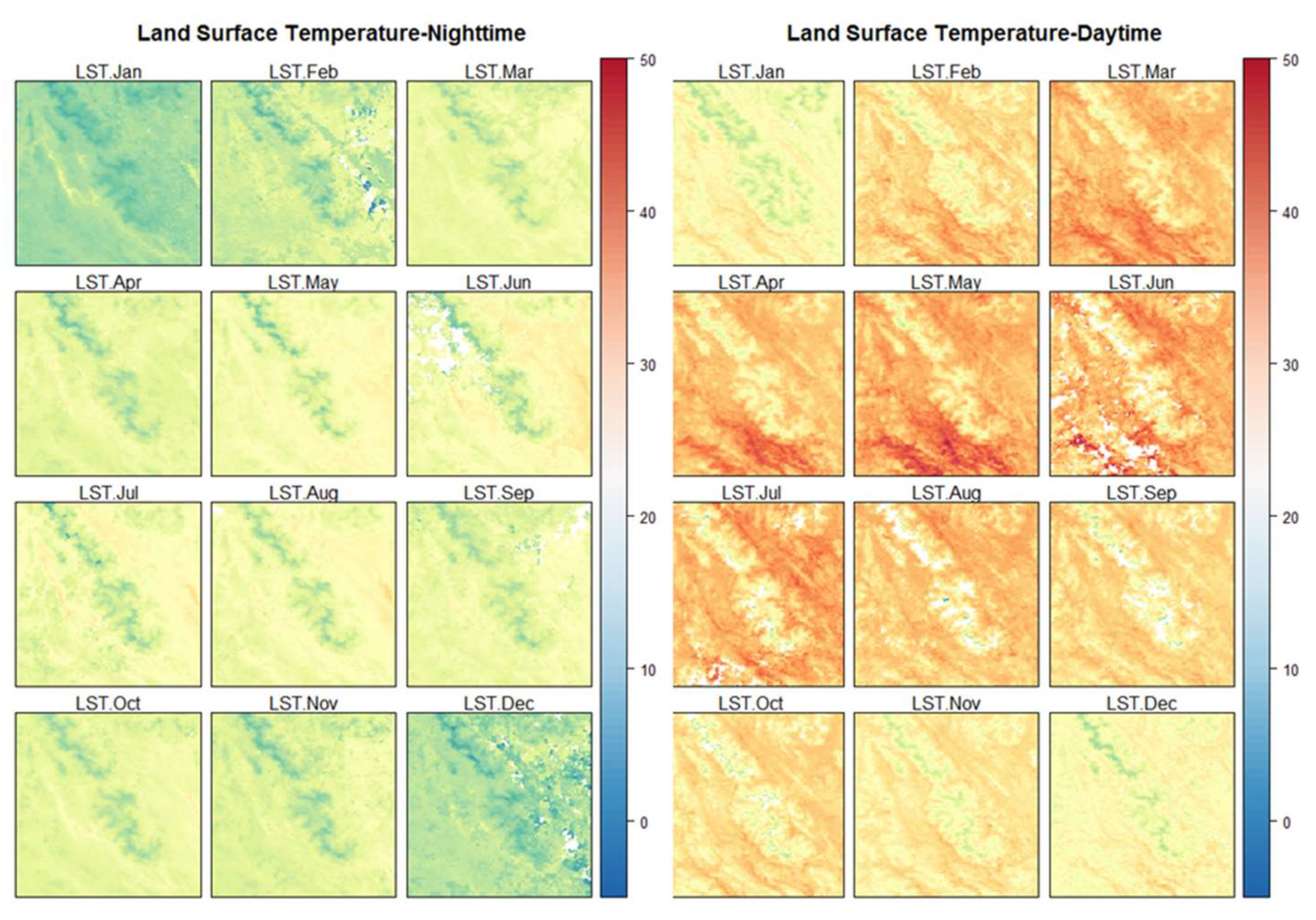
Figure 3.
Violin plots show the monthly average LST of the daytime (top) and nighttime (bottom) in 2015 in northwest Vietnam.
Figure 3.
Violin plots show the monthly average LST of the daytime (top) and nighttime (bottom) in 2015 in northwest Vietnam.
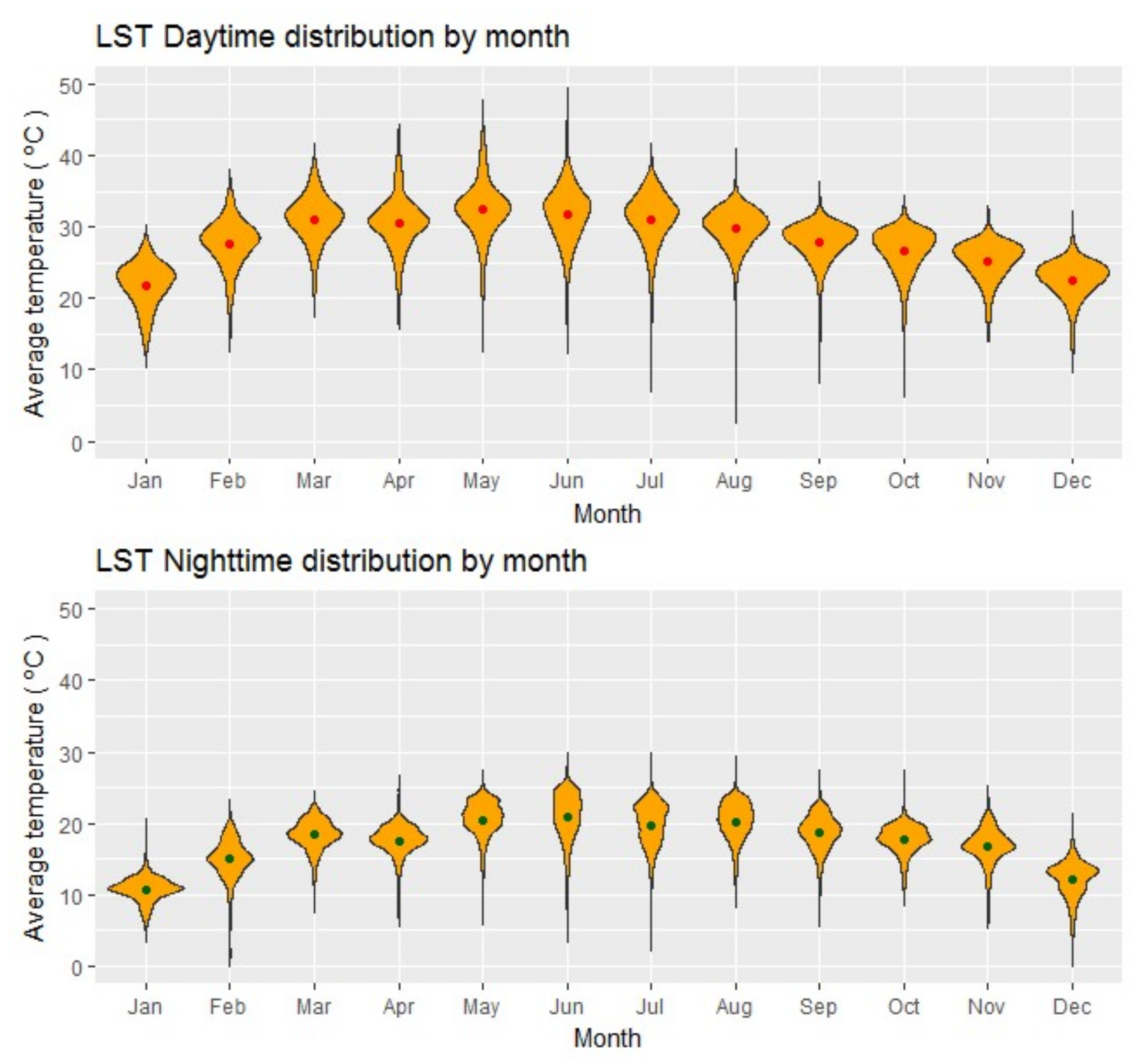
Figure 4.
(a) Scatter plots showing the relationship between average monthly daytime LST (D-LST) and elevation in northwest Vietnam in 2015. (b) Scatter plots showing the relationship between average monthly nighttime LST (N-LST) and elevation in northwest Vietnam in 2015. The color ramp from blue to red expresses the point density from low to high.
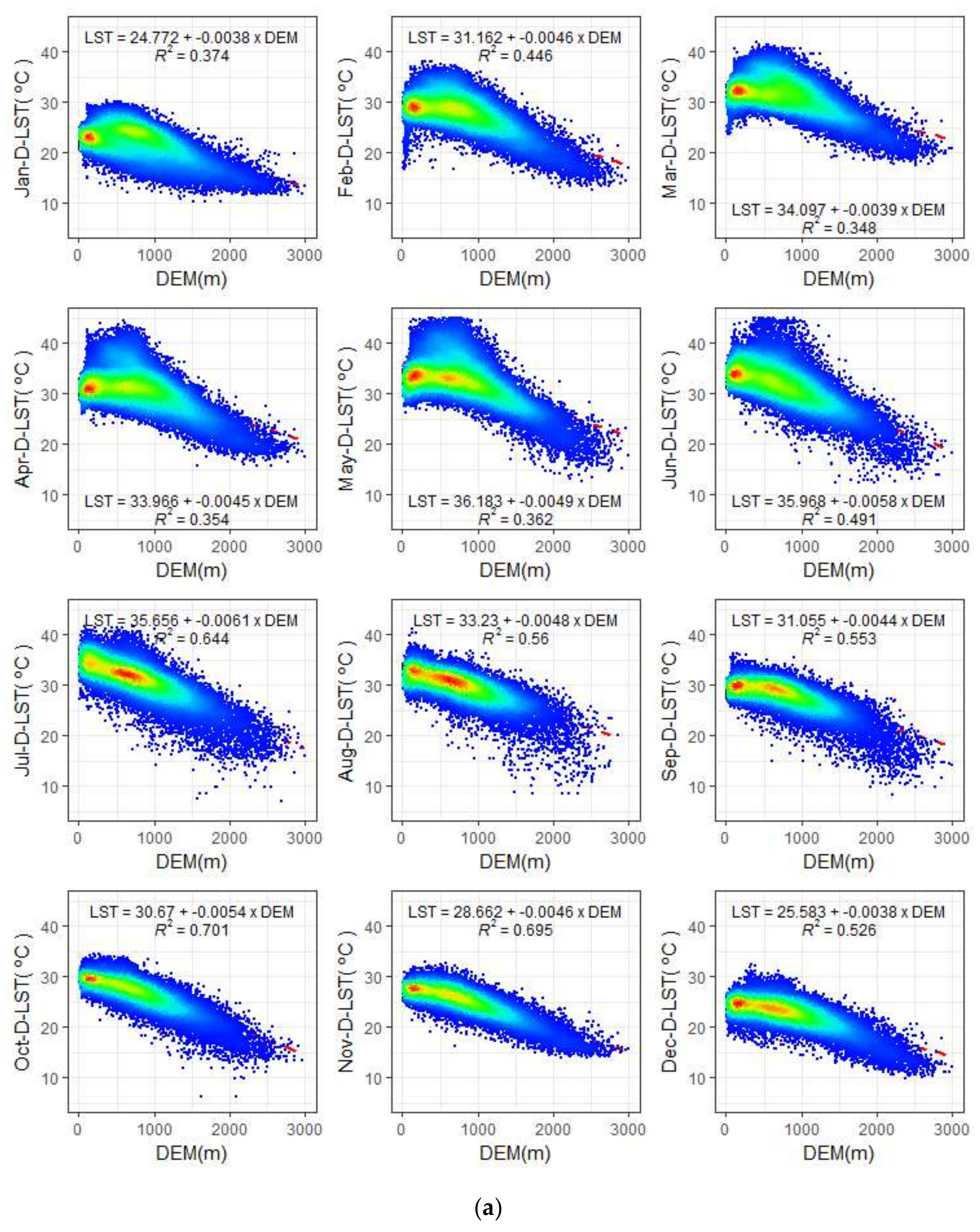
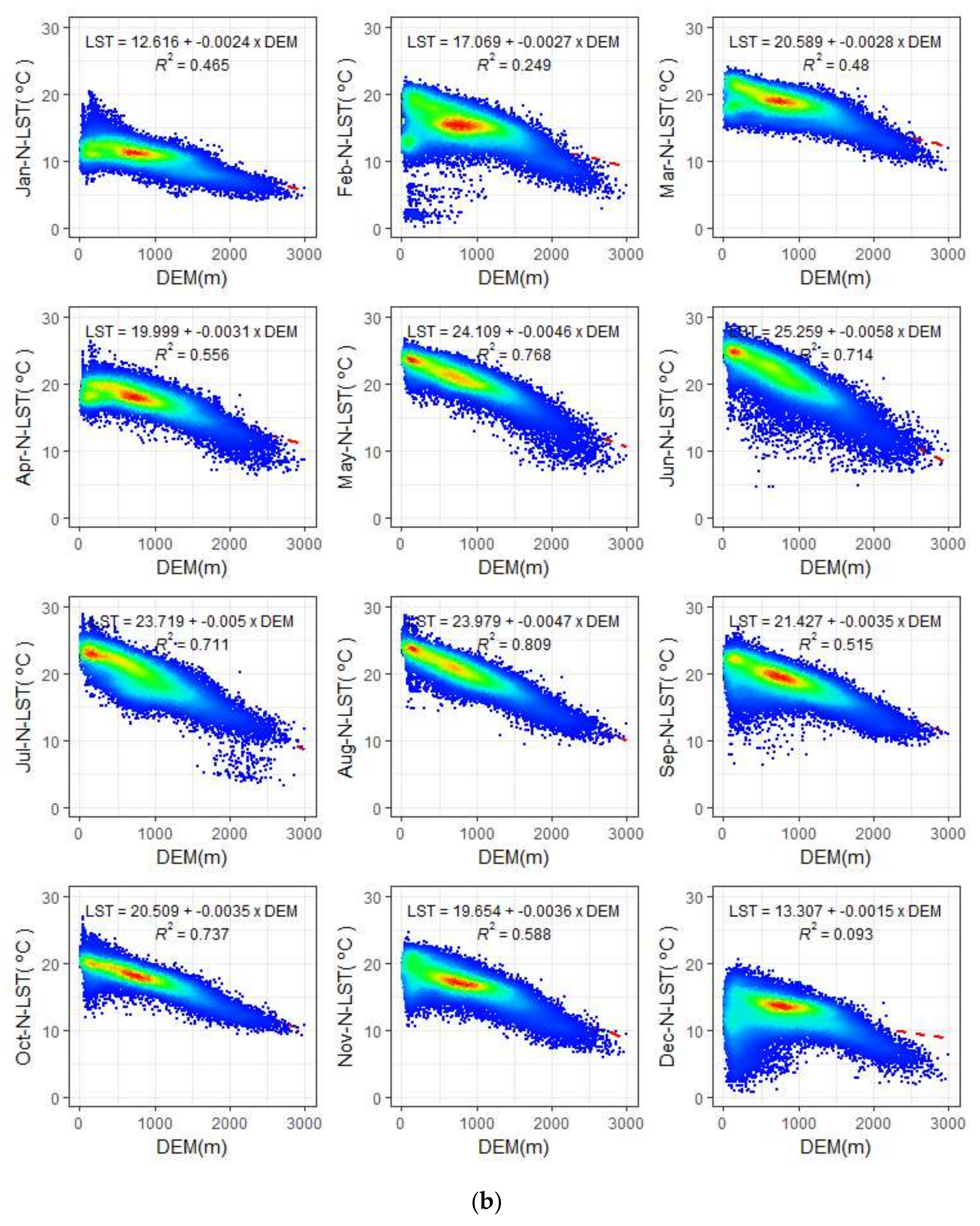
Figure 5.
(a) Scatter plots showing the relationship between average monthly daytime LST of different land cover types and elevation in northwest Vietnam in 2015. (b) Scatter plots showing the relationship between average monthly nighttime LST of different land cover types and elevation in northwest Vietnam in 2015. The color ramp from blue to red expresses the point density from low to high.
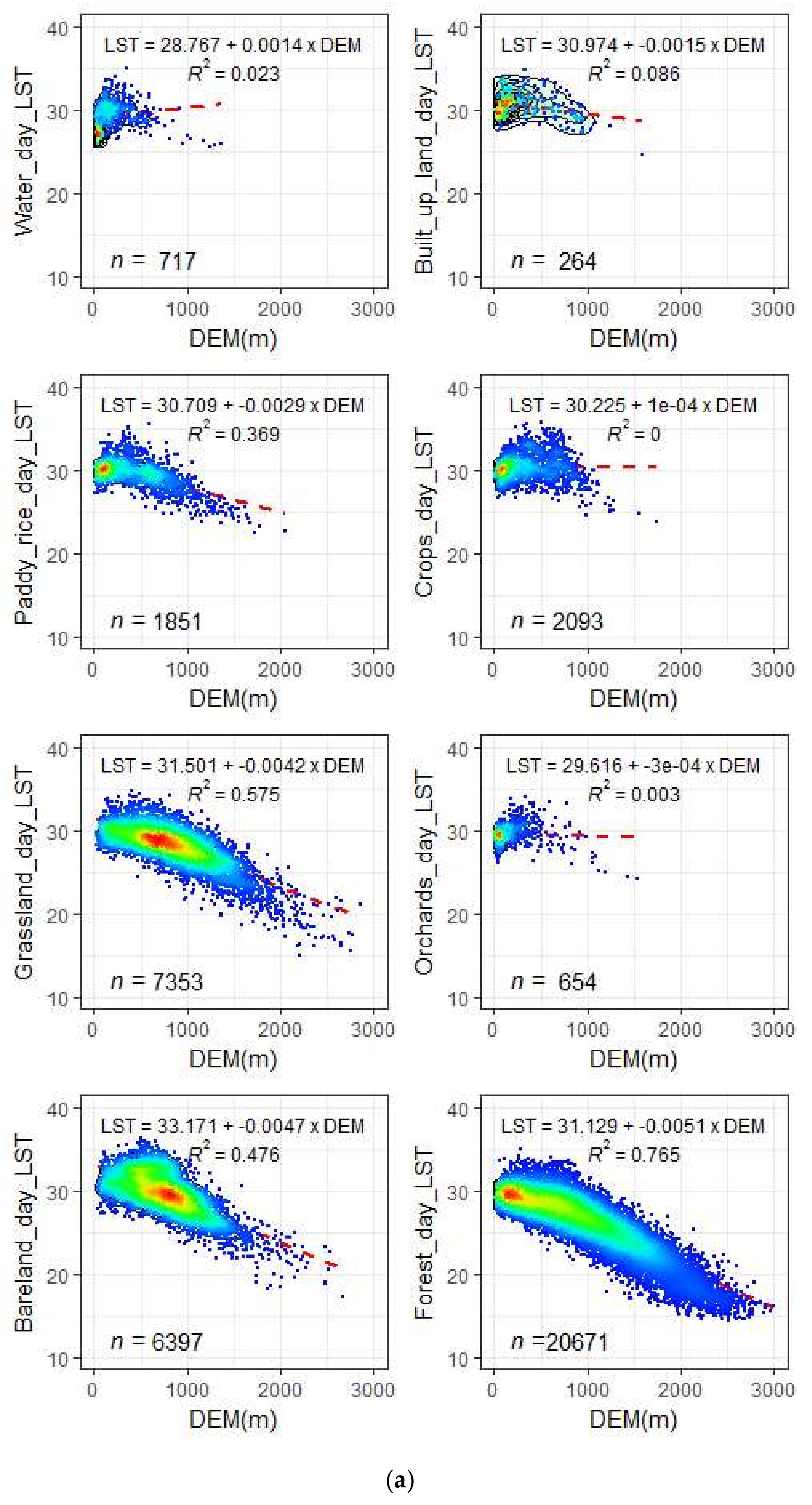
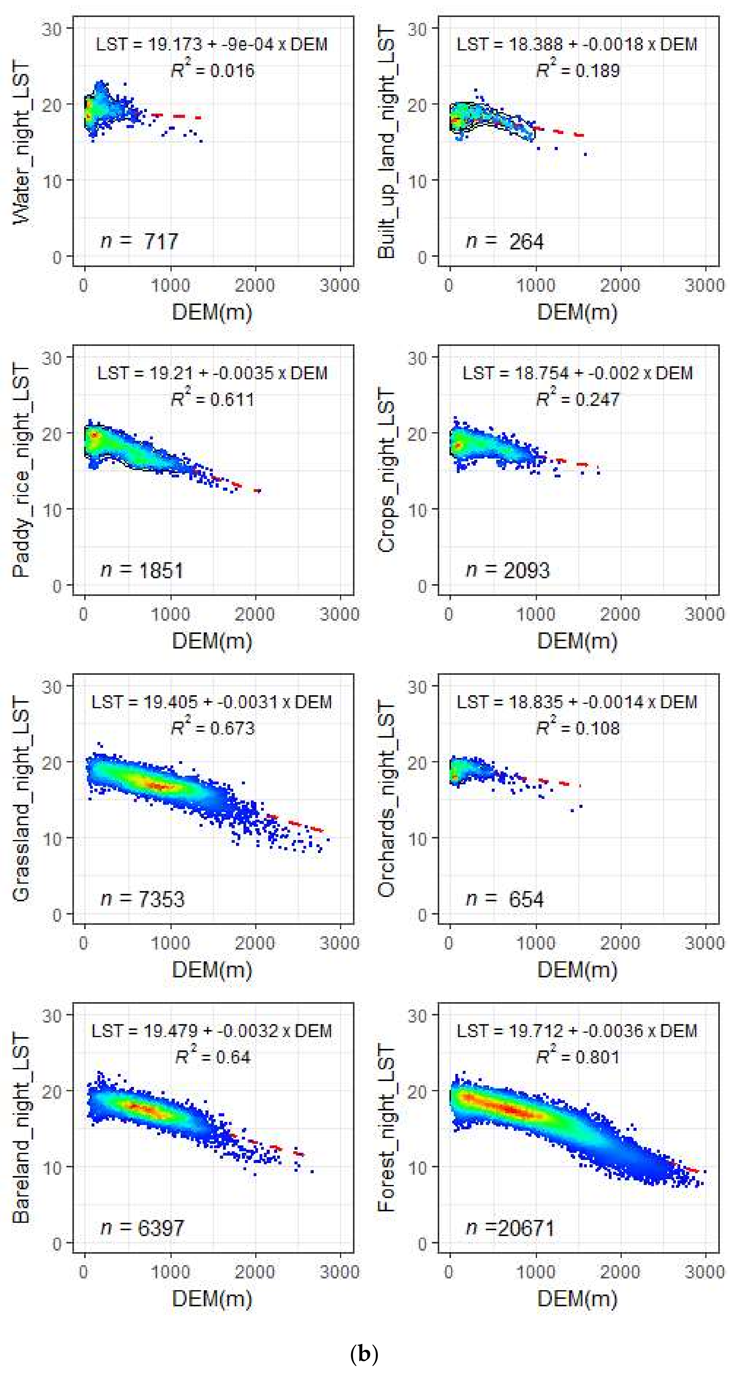
Figure 6.
(a) Scatter plots showing the relationship between the average monthly daytime LST of a balanced number of observation-based elevations and the elevation in northwest Vietnam in 2015. (b) Scatter plots showing the relationship between the average monthly nighttime LST of a balanced number of observation-based elevations and the elevation in northwest Vietnam in 2015. The color ramp from blue to red expresses the point density from low to high.


Figure 7.
(a) Scatter plots showing the relationship between the average monthly LST (daytime and nighttime) and elevation of Lane 1 in 2015. (b) Scatter plots showing the relationship between the average monthly LST (daytime and nighttime) and elevation of Lane 2 in 2015. The color ramp from blue to red expresses the point density from low to high.

© 2018 by the authors. Licensee MDPI, Basel, Switzerland. This article is an open access article distributed under the terms and conditions of the Creative Commons Attribution (CC BY) license (http://creativecommons.org/licenses/by/4.0/).
Share and Cite
MDPI and ACS Style
Phan, T.N.; Kappas, M.; Tran, T.P. Land Surface Temperature Variation Due to Changes in Elevation in Northwest Vietnam. Climate 2018, 6, 28. https://doi.org/10.3390/cli6020028
AMA Style
Phan TN, Kappas M, Tran TP. Land Surface Temperature Variation Due to Changes in Elevation in Northwest Vietnam. Climate. 2018; 6(2):28. https://doi.org/10.3390/cli6020028
Chicago/Turabian StylePhan, Thanh Noi, Martin Kappas, and Trong Phuong Tran. 2018. "Land Surface Temperature Variation Due to Changes in Elevation in Northwest Vietnam" Climate 6, no. 2: 28. https://doi.org/10.3390/cli6020028
Note that from the first issue of 2016, this journal uses article numbers instead of page numbers. See further details here.